


Abstract
We present elemental abundance data of C, N, O, Na, Mg, Al, Ca, and Cr in Genesis silicon targets. For Na, Mg, Al, and Ca, data from three different solar wind (SW) regimes are also presented. Data were obtained by backside depth profiling using secondary ion mass spectrometry. The accuracy of these measurements exceeds those obtained by in situ observations; therefore, the Genesis data provide new insights into elemental fractionation between Sun and SW, including differences between SW regimes. We integrate previously published noble gas and hydrogen elemental abundances from Genesis targets, as well as preliminary values for K and Fe. The abundances of the SW elements measured display the well-known fractionation pattern that correlates with each element's first-ionization potential (FIP). When normalized either to spectroscopic photospheric solar abundances or to those derived from CI-chondritic meteorites, the fractionation factors of low-FIP elements (K, Na, Al, Ca, Cr, Mg, Fe) are essentially identical within uncertainties, but the data are equally consistent with increasing fractionation with decreasing FIP. The elements with higher FIPs between ∼11 and ∼16 eV (C, N, O, H, Ar, Kr, Xe) display a relatively well-defined trend of increasing fractionation with decreasing FIP, if normalized to modern 3D photospheric model abundances. Among the three Genesis regimes, the fast SW displays the least elemental fractionation for almost all elements (including the noble gases) but differences are modest: for low-FIP elements, the precisely measured fast–slow SW variations are less than 3%.
Export citation and abstract BibTeX RIS
1. Introduction
NASA's Genesis spacecraft collected solar wind (SW) ions for laboratory analysis with the goal of obtaining high-precision isotopic and elemental abundances of solar matter. In order to constrain the amounts of fractionation between the SW and the photosphere, aside from the bulk SW, the mission sampled three different SW regimes: interstream (slow), coronal hole (fast), and coronal mass ejections (CME; Neugebauer et al. 2003; Burnett & Genesis Science Team 2011; Burnett 2013; Reisenfeld et al. 2013). To meet the mission goals, the accuracy of the measurement is required to meet the needs of planetary science.
So far, these goals have been fully or largely achieved for noble gases (e.g., Grimberg et al. 2006; Meshik et al. 2007, 2014, 2020; Heber et al. 2009; Vogel et al. 2011, 2019; Pepin et al. 2012; Crowther & Gilmour 2013), with only Kr and Xe isotopic composition data from regime targets missing. Isotopic data are also available for O and N in bulk SW, the two highest priorities of Genesis (Marty et al. 2010, 2011; McKeegan et al. 2011; Huss et al. 2012) and Mg (Jurewicz et al. 2020). Hydrogen fluences in bulk SW and regime targets were published by Huss et al. (2020). For a number of other elements important for cosmochemistry, elemental abundances in bulk SW targets have been published in preliminary form (Heber et al. 2013, 2014b, 2014c; Rieck 2015; Rieck et al. 2016; Burnett et al. 2017).
For the first time, this work presents comprehensive elemental abundance data for four cosmochemically important elements in Genesis bulk SW and regime targets: Na, Mg, Al, and Ca. We also present our final abundance data of C, N, O, and Cr for bulk SW targets. We put these data into perspective by calculating the extent of elemental fractionation between the Sun and SW, with a special emphasis on the elements for which SW abundances in the different regimes are available. All data were obtained by secondary ion mass spectrometry (SIMS) using backside depth profiling. Some details of this technique will be briefly explained in the next section; for a full description, see Heber et al. (2014a).
It is well known that elemental fractionation upon SW formation correlates with the first-ionization potential (FIP) of the elements (e.g., Pilleri et al. 2015). Elements with low FIP (below some 9–10 eV) are overabundant relative to O in the SW by a factor of a few. The elements measured in this work for which regime data are available are all low-FIP elements, ranging from 5.14 eV (Na) to 7.65 eV (Mg), whereas C, N, and O, for which we present bulk SW fluences, have high FIPs, between 11.3 and 14.5 eV. For a better understanding of the underlying fractionation mechanisms, we therefore also consider in the discussion the fluence data for high-FIP elements for which Genesis regime data are available, in particular noble gases (Heber et al. 2009, 2012; Vogel et al. 2019) and hydrogen (Huss et al. 2020). We also include data for K (Rieck 2015; Rieck et al. 2016) and Fe (Burnett et al. 2017) in bulk SW targets.
In Section 2, we will discuss the analytical technique of analyzing concentrations of elements implanted by the SW in Genesis targets. In Section 3, we will present the main experimental results, and in Section 4, we will discuss these data in terms of SW fractionation effects as well as solar elemental abundances.
2. Experimental
Fluences of implanted SW elements were analyzed by backside depth profiling using SIMS. This method is widely employed in the semiconductor industry to analyze depth distributions of dopant elements (e.g., Zinner 1983). In this work, SW-bearing silicon wafers of 0.55–0.7 mm thickness were glued upside down onto a Si substrate and then thinned mechanically from the backside. Heber et al. (2014a) showed that the optimal thickness of the thinned SW collectors is about 800 nm. They discuss the importance of obtaining a highly plane-parallel polish in order to obtain a reasonably large flat central area, allowing them to obtain SW profiles until close to the collector surface.
Depth profiling from the backside was performed with two different SIMS instruments (Heber et al. 2014a). This technique largely avoids two major problems encountered by conventional SIMS when analyzing very low quantities of the species of interest implanted at very shallow depths of a few tens of nanometers, as is the case for Genesis targets. First, atomic mixing (knock-on) of ions from a high-abundance surface contaminant can mask the signal of interest and may result in erroneously high fluences of the SW elements. This process is not absent in backside depth profiling but is much less important. Second, at the onset of the sputtering process, secondary ion yields vary markedly in the first ∼10 nm or so, seriously affecting the determination of the most surficial part of SW implantation profiles. Heber et al. (2014a) demonstrated that with backside depth profiling, nearly complete profiles of many SW elements in Genesis targets can be obtained. That paper gives a full account of the specific experimental methods used to obtain the data presented here. In the following, we give a brief summary.
2.1. Samples and Sample Preparation
Due to the crash landing of the Genesis sample return capsule, all SW-bearing sample wafers (originally 10 cm hexagons of a variety of materials and surface coverings) were shattered to small pieces and contaminated by particles from the Utah desert (Burnett & Genesis Science Team 2011). For all analyses here, fragments of float-zone (FZ) silicon wafers (on the order of 8 × 8 mm) were chosen. All fragments were very carefully cleaned of Utah dust (Allton et al. 2007; Calaway et al. 2007) before being glued onto the Si substrate (Table 4 in Appendix A.1 for sample numbers). The elements C, N, O, and Cr were analyzed only in samples exposed to bulk SW targets during the entire ∼2.3 yr duration of the Genesis collection period, whereas, in addition to bulk SW, Na, Mg, Al, and Ca were also measured in regime samples. The "fast" and "slow" regimes were sampled for slightly more than 300 days each, CMEs for ∼190 days. Reisenfeld et al. (2007, 2013) and Neugebauer et al. (2003) give details about the Genesis regime selection and SW properties during the different regimes. There is an overlap in fast SW and slow SW speed intervals as defined by the regime selection algorithm, essentially in the range between ∼400 and 540 km s−1, while the CME targets also sampled at least ∼25% of non-CME SW (Reisenfeld et al. 2013).
2.2. SIMS Analytical Techniques
The elements Na, Mg, Al, Ca, and Cr were analyzed with the Cameca IMS 1270 at the University of California, Los Angeles, and C, N, and O with the Cameca 7f-Geo at the California Institute of Technology, Pasadena. A low-energy primary ion beam (5 keV 133Cs+ for negative secondary ions of C, N, and O and 7 keV  for positive secondary ions of Na, Mg, Al, Ca, and Cr) was rastered over, in most cases, a 100 μm × 100 μm area. The low energy of the primary ions was chosen to reduce knock-on, thereby improving depth resolution. Sputter rates ranged between 0.1 and 0.25 nm s−1. Secondary ions sputtered from the center of the raster were selected using a field aperture that physically masks ions from outside the transmitted area. The mass resolving power was chosen to resolve all significant molecular ion interferences from the signal of interest. Isotopes were analyzed by magnetic field peak switching using an electron multiplier for the implanted isotopes and a Faraday cup for the matrix element Si.
2.3. Sample Analysis
The thinned Si SW collectors were sputtered from the backside with minor modifications from traditional backside-sputtering techniques used by the semiconductor industry (see Heber et al. 2014a for details). In most cases, only one element of interest was analyzed per session, to maximize the data coverage during a depth profile. Due to their similar masses, Mg and Na require lower waiting times upon peak switching and thus these two elements were analyzed in the same session. Figure 1 shows, for each element, one measured backside depth profile.

Figure 1. Examples of measured and extrapolated solar wind profiles of different elements in bulk SW targets or different SW regimes (sample details given in Tables 4 and 5 in Appendix). Ordinates represent concentrations in 1016 ions cm−3, abscissae the depth in nanometers measured from the backside surface of the collector. Measured solar wind data are shown as orange squares, red dots represent data at and after breakthrough, i.e., when the primary ion beam first penetrates the collector surface. The polynomial fit of the extrapolation of the profiles prior to breakthrough is shown as black solid line.
Download figure:
Standard image High-resolution imageDetails on data reduction techniques and fluence calibrations are given by Heber et al. (2014a) and summarized in Appendices A.1 and A.2.
2.4. Uncertainties
Stated 1σ uncertainties of the mean SW fluence of elements given in Table 1 include the standard deviation of all fluence measurements and the mean uncertainties of all relative sensitivity factors (RSFs) and sputtering rates (S) (Appendix A.1, Table 4). The total uncertainty of the mean bulk SW fluence includes the uncertainty of the absolute calibration and 10% for N and Al, which are not calibrated.
Table 1. Solar Wind Element Fluences Measured in Genesis Collectors
| Element | FIP (eV) | Solar Wind Fluence (ions cm−2) | |||||||||
|---|---|---|---|---|---|---|---|---|---|---|---|
| bulk | ± | Total Error | Slow | ± | Fast | ± | CME | ± | Reference | ||
| C | 11.26 | 6.41E12 | 0.32E12 | 0.37E12 | |||||||
| N | 14.53 | 1.23E12 | 0.03E12 | 0.13E12 | |||||||
| O | 13.61 | 1.17E13 | 0.12E13 | 0.12E13 | |||||||
| Na | 5.14 | 1.23E11 | 0.04E11 | 0.08E11 | 5.18E10 | 0.10E10 | 3.36E10 | 0.17E10 | 3.25E10 | 0.09E10 | |
| Mg | 7.65 | 1.73E12 | 0.04E12 | 0.06E12 | 7.19E11 | 0.14E11 | 4.82E11 | 0.11E11 | 4.56E11 | 0.07E11 | |
| Al | 5.99 | 1.42E11 | 0.05E11 | 0.15E11 | 5.54E10 | 0.24E10 | 3.69E10 | 0.10E10 | 3.80E10 | 0.15E10 | |
| Ca | 6.11 | 1.17E11 | 0.04E11 | 0.06E11 | 4.80E10 | 0.05E10 | 3.19E10 | 0.05E10 | 3.31E10 | 0.02E10 | |
| Cr | 6.77 | 2.32E10 | 0.05E10 | 0.11E10 | |||||||
| H | 13.6 | 1.634E16 | 0.014E16 | 0.164E16 | 0.624E16 | 0.022E16 | 0.551E16 | 0.006E16 | 0.412E16 | 0.015E16 | 1 |
| He | 24.58 | 8.293E14 | 0.022E14 | 0.15E14 | 3.152E14 | 0.012E14 | 2.597E14 | 0.006E14 | 2.532E14 | 0.008E14 | 2 |
| Ne | 21.56 | 1.359E12 | 0.006E12 | 0.032E12 | 5.292E11 | 0.028E11 | 4.447E11 | 0.020E11 | 3.864E11 | 0.016E11 | 2 |
| Ar | 15.75 | 3.547E10 | 0.017E10 | 0.070E10 | 1.398E10 | 0.007E10 | 1.200E10 | 0.013E10 | 0.928E10 | 0.006E10 | 2 |
| Kr | 13.99 | 2.20E7 | 0.12E7 | 0.16E7 | 8.66E6 | 0.10E6 | 7.47E6 | 0.13E6 | 5.64E6 | 0.07E6 | 3 |
| Xe | 12.13 | 4.87E6 | 0.29E6 | 0.38E6 | 1.83E6 | 0.04E6 | 1.39E6 | 0.06E6 | 1.19E6 | 0.06E6 | 3 |
Note. Isotopic compositions used to calculate element fluences from measured data are from Heber et al. (2009) for He, Ne, and Ar; Meshik et al. (2014, 2020) for Kr and Xe; McKeegan et al. (2011) for O; and Marty et al. (2011) for N. Terrestrial values adopted for C, Mg, Ca, and Cr. Noble gas fluences were recalculated from original references (see Appendix A.4). Stated uncertainties are 1σ (including those of H from reference (1); total error for H in bulk SW includes 10% uncertainty of H2O concentration in apatite standard). Errors in columns "±" do not include the systematic uncertainties of the standards, because these cancel when comparing differences in fluences and element ratios among different regimes. The total error including errors in standard calibration is shown for the bulk fluences. Exposure durations: bulk SW = 852.83 days, fast SW = 313.01 days, slow SW = 333.67 days; CME = 193.25 days (Reisenfeld et al. 2013).
References. (1) Huss et al. (2020), (2) Heber et al. (2009), (3) Vogel et al. (2019).
Download table as: ASCIITypeset image
3. Results
The mean SW fluences for each element (and each regime, when available) are given in Table 1. The table also shows noble gas fluences for bulk SW and Genesis regimes, slightly updated from those given by Heber et al. (2009) and Vogel et al. (2019), with details explained in Appendix A.4. The H fluences are those from Huss et al. (2020) measured by SIMS in Genesis targets. Uncertainties (1σ) for bulk fluences include uncertainties of standards (Heber et al. 2014a; Vogel et al. 2019; Huss et al. 2020). Uncertainties of regime data do not include the systematic uncertainties of the standards, because these cancel when comparing differences in fluences and element ratios in different regimes. The complete data collected during this study is given in Table 4 in Appendix A.1.
The exposure-duration-weighted sum of regime fluences should be the same as the bulk fluence. The calculated bulk fluences agree within uncertainties with the values measured in bulk SW targets: summed regime fluences amount to 97%, 97%, 93%, and 98% of the bulk collector values for Na, Mg, Al, and Ca, respectively. For comparison, the weighted total regime fluence of H measured by Huss et al. (2020) amounted to 99% of their bulk SW target value, if the slightly lower total exposure durations of the three regime arrays are taken into account.
4. Discussion
4.1. Low-FIP Elements
Figure 2 shows the ratios of the relative fluences (element/Mg) measured in Genesis bulk SW (Figure 2(a)) and regime targets (Figure 2(b)) after normalization to the respective solar abundance ratios (Table 7 in Appendix A.5). The bulk SW data for K and Fe in silicon (marked by asterisks in Figure 2(a)) are the preliminary fluences from Rieck (2015), Rieck et al. (2016), and Burnett et al. (2017). If SW had the composition of the solar photosphere, the ordinate value in Figure 2 would be 1 for all elements. The bulk SW shows a fractionation of elemental abundances correlating with FIP, as previously observed by spacecraft (e.g., Geiss 1982; Bochsler 2009). However, the better accuracy and element coverage of Genesis data compared to in situ measurements allows further insights into this FIP-related fractionation. The low-FIP elements (Figure 2(a)) are consistent with a flat pattern, at least below 7 eV, as many pre-Genesis studies suggested. This consistency would make these SW data easier to apply to cosmochemistry, as they would suggest that low-FIP elements are unfractionated relative to each other and hence their SW abundance ratios equal photospheric ratios. However, Figure 2(a) is also consistent with a monotonic increase of the low-FIP elements with decreasing FIP, which could be viewed as a trend continuing that of the high-FIP elements between Ar and C discussed below. The Na abundance given here is about 20% higher than that of Burnett et al. (2017). Na fluences derived from backside depth profiling of diamond-like-C collectors are roughly a factor of 2 lower than ours, which are based on Si collectors (Rieck 2015; Rieck et al. 2016). Jurewicz et al. (2019) propose that diffusion of surface contamination Na might have enhanced fluences from Si collectors. Because the amounts of surface contamination is highly variable, the Na fluences from Si should show significant scatter; however, replicate analyses of bulk and regime samples agree to within 2%–11% (Table 4, Appendix A.1). More analyses are required to resolve this important discrepancy. A ∼20% lower fractionation of K compared to that of Na, if real, would be surprising although within 2σ, both values still overlap.
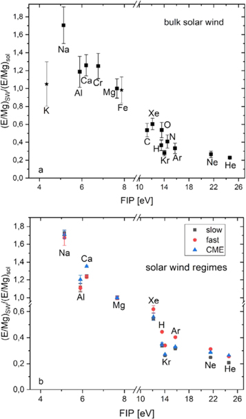
Figure 2. (a) (Upper panel): fluence ratios (elements/Mg) in Genesis bulk SW targets normalized to solar ratios (Table 7, Appendix A.5). Values from this work and H are from Table 1. Data for K (Rieck 2015) and Fe (Burnett et al. 2017) in bulk SW targets (a) are shown by asterisks. Error bars for bulk targets reflect the total uncertainties given in Table 1 and 1σ uncertainties of solar ratios. (b) (Lower panel): fluence ratios (elements/Mg) in Genesis regime targets. Here, only the analytical uncertainties (± in Table 1), with uncertainties for Mg not propagated, are shown. The FIPs of some elements in panel (b) are slightly shifted to increase visibility. Ordinate data are shown in Table 8 (Appendix A.5). The FIP plots for the different regimes are strikingly similar, particularly for low-FIP elements. Fast SW has been regarded as the least fractionated. Our results confirm this, but the decrease in fractionation is relatively small.
Download figure:
Standard image High-resolution imageInefficient Coulomb drag (Bodmer & Bochsler 2000) would not predict such a difference in fractionation between two elements of almost equal mass (K and Ca). These elements are expected to have a similar charge state distribution; moreover, the difference would also run opposite to the possible increase of fractionation with decreasing FIP mentioned above. The final Genesis-derived abundance of K will be important in this comparison.
The FIP fractionation pattern predicted by the model of Laming et al. (2017, 2019) is in reasonable agreement with the low-FIP element data in Figure 2(a). This model explains FIP fractionation by the ponderomotive force in the chromosphere. Conservation of the adiabatic invariant during acceleration away from the photosphere is invoked to account for isotope fractionation.
Figure 3 shows an FIP trend of SW element/Mg ratios normalized to the values in CI carbonaceous chondrites instead of photospheric spectroscopic abundances. Elemental abundances in CI chondrites (e.g., Lodders 2020) are often used as a surrogate of solar abundances for most elements, because of the overall agreement between CI and photospheric values derived by spectroscopy when available. On the other hand, solar abundances should be based on data from the Sun: to clarify the validity of CI abundances as a proxy for solar values is one of the ultimate goals of Genesis. At this point, we note that the apparent fractionation factors element/Mg in Figure 3 show a slightly smaller spread than those in Figure 2(a), with all ratios agreeing within better than 25% with CI values.

Figure 3. Fluence ratios (elements/Mg) in Genesis bulk SW and fast SW targets normalized to respective ratios in CI chondrites (Lodders 2020). Error bars for bulk targets reflect the total uncertainties given in Table 1 and 1σ errors for CI chondrites. Error bars for fast SW reflect only analytical uncertainties (± in Table 1). For clarity, besides bulk SW data, only those for the fast SW regime, thought to be the least fractionated, are shown, but the good agreement with CI abundances also holds for the other two regimes.
Download figure:
Standard image High-resolution imageFigure 2(b) shows the fractionation patterns of the different Genesis regime targets as a function of FIP, again with Mg as the normalizing element. In situ data generally reveal that the fractionation between low-FIP and high-FIP elements is less for fast than slow SW (e.g., von Steiger et al. 2000; Bochsler 2009). This is also observed in Figure 2(b), i.e., the fast SW fractionation factors are closer to 1 (lower for low-FIP elements and higher for high-FIP elements). Most importantly, for low-FIP elements, differences in normalized element/Mg ratios are small, not more than 10% between CME and fast SW and even less between slow SW and fast SW. These differences are significant beyond the 1σ level only for Ca and (marginally) Al in CME targets. In particular, the Na/Mg ratio shows the smallest spread among the low-FIP elements, perhaps contrary to expectations, given that Na appears to show the strongest fractionation in the bulk SW among all elements shown in Figure 2(a).
Even given the overlap in SW speeds actually sampled by the fast- and slow-SW regimes, the close similarity of the low-FIP fractionation patterns in Figure 2(b) is new and potentially important. This has not been recognized by previous studies of SW composition primarily because of the high precision possible in interregime comparisons of element ratios in our data (Table 2). The major source of errors in the fractionation factor (implant standard calibrations and the spectroscopic photospheric abundances) do not enter into the comparison of the regime data. The analytical precision of the ratios in Table 2 is 1.6%–4.6%. As noted above, significant interregime differences (4.8%–11.2%) are observed, but the important point is that these are small, especially between fast and slow regimes. The fast and slow SW form by different mechanisms in different solar environments (e.g., Neugebauer & von Steiger 2001; Laming et al. 2017). Consequently, it seems unlikely that fractionations among low-FIP elements would be the same for both fast and slow as shown in Table 2. This is possibly an indirect, but potentially strong, argument that there are no significant fractionations among the low-FIP elements as a set (i.e., a flat pattern on Figure 2). There, of course, is still the larger fractionation between high- and low-FIPs, which is a separate issue. Nonfractionation among low-FIP elements might only hold below about 7 eV. Pilleri et al. (2015) propose, based on processing ACE-SWICS data for the Genesis period, that there is a non-FIP mass-dependent fractionation between Mg and Fe. As discussed in Appendix A.6, our result is fully compatible with previous SW composition data sets. The widely recognized smaller fractionation of fast SW is primarily a smaller difference between low-FIP and high-FIP elements taken as groups, specifically between low-FIP elements and O.
Table 2. Comparison of Low-FIP Element Ratios in Genesis Regimes
| Regime | Na/Mg | Al/Mg | Ca/Mg |
|---|---|---|---|
| Slow | 0.0716 | 0.0771 | 0.0668 |
| Fast | 0.0697 | 0.0766 | 0.0662 |
| CME | 0.0597 | 0.0833 | 0.0726 |
| Average regimes | 0.0664 | 0.0790 | 0.0685 |
| stdev (%) | 11.2% | 4.8% | 5.2% |
| Bulk | 0.0711 | 0.0821 | 0.0676 |
Note. Errors in individual element/Mg values are 1.6%–4.6%.
Download table as: ASCIITypeset image
Figure 4 shows flux ratios in Genesis regimes over those in bulk SW. This format is independent of assumed solar compositions as well as of absolute calibration uncertainties when interregime comparisons are being made. First, we note that the observation based on noble gases (Vogel et al. 2019) that fluxes increase in the order fast–slow–CME also holds for the low-FIP elements. Furthermore, three different groupings are observed: (i) the low-FIP elements show substantially different fluxes in the different regimes, (ii) fluxes for H, Kr, and Ar are similar within 20% in all three regimes, and (iii) He and Ne again show large differences. There also appears to be a crossover pattern, in that the flux differences between fast SW and CMEs first seem to decrease with increasing FIP, while they clearly increase again for the two highest FIP elements Ne and He.
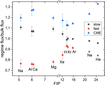
Figure 4. Ratios of elemental fluxes in Genesis regimes over those in Genesis bulk solar wind (bulk solar wind data obtained from weighted regime target data). Data from Table 1.
Download figure:
Standard image High-resolution image4.2. High-FIP Elements
In Figure 2(a), the data for C, N, and O (and H) for bulk SW fit into the noble gas pattern already discussed by Vogel et al. (2019). For both bulk and regime SW samples, these high-FIP elements display the above-mentioned trend of increasing normalized abundances with decreasing FIP in the 15−11 eV region between Ar and C (see also Meshik et al. 2020). Abundance ratios Xe/Kr and Xe/Ar higher than solar in the SW were already observed based on lunar regolith data (Wieler & Baur 1995; Wieler et al. 1996). Geiss & Bochsler (1985) proposed to explain this enhancement of Xe to be due to the fact that in the SW source region, Xe has a relatively low first-ionization time (FIT), the characteristic time for an element to undergo its first ionization in the chromosphere, a parameter closely related to FIP. Xenon indeed has the lowest FIT of all elements between 15 and 11 eV shown in Figure 2(a). However, otherwise there is no conspicuous dependence of the fractionation factors of these elements on FIT, indicating that FIT is not the most relevant parameter governing the SW abundance pattern in the high-FIP region below Ne.
The position of the CNO points in Figure 2(a) is also relevant for the discussion of solar elemental abundances of these three elements (e.g., Serenelli et al. 2016; von Steiger & Zurbuchen 2016). Note that the position of the Kr and Xe points relative to that of H is well constrained as (i) Kr and Xe abundances in the SW are well known, thanks to the precise noble gas data (including He) provided by Genesis and the accurate He abundance provided by helioseismology and (ii) solar Kr and, to a lesser extent, Xe abundances can be derived with high confidence, Kr by interpolating meteoritic abundances of neighboring elements, Xe from nucleosynthesis theory (see Table 7 in Appendix A.5 and Meshik et al. 2020). The fact that the CNO points in Figure 2(a) display the same trend as H, Kr, and Xe is, thus, an argument in favor of the solar abundances of CNO used here, which are those given by Asplund et al. (2009). This speaks against the suggestion by Laming et al. (2017) that the difference between their modeled fractionations and the measured data in the high-FIP region may indicate an underestimation of the solar O and N abundances by Asplund et al. (2009).
The high-FIP elements show systematic differences in the different regimes (Figure 2(b)). Their abundances relative to Mg are more fractionated in CME and slow SW than in the fast SW (i.e., fast SW data points plot closest to the 1:1 line). Relative differences are modest, yet tend to be somewhat larger than those for the low-FIP elements (e.g., ∼28% for Ar/Mg in fast versus slow wind). The only exception to this is He, where the CME point falls marginally above that of fast SW. In terms of He/H the CME ratio is about 25%–30%% higher than slow or fast (Huss et al. 2020, Figure 18). Figure 4 shows that relative fluxes of Ne and especially He increase markedly in CMEs (by about 16% in the case of He), which is compensated by a roughly parallel decrease of the relative fluxes of these two elements in fast and slow SW (see also Vogel et al. 2019). High He/H is observed in some CME events (Borrini et al. 1982). It is also worth noting that the Genesis CME sample is basically all ions that were not clearly fast or slow SW and could contain several different sources of high He SW. High He/H was one, but only one, of the factors that triggered the deployment of the Genesis CME array.
Also notable on the high-FIP side of Figure 4 are two further observations. First, in all three regimes, the Kr flux closely follows H, which has a very similar FIP. Second, whereas the slow regime shows a monotonic decrease with FIP from Mg to He, in the fast SW, Xe, H, and Kr increase markedly relative to Mg. These observations further indicate that the fractionation of the high-FIP elements in the SW is governed by more than the FIP.
4.3. Comparing Genesis-derived Elemental Abundances with in Situ Data
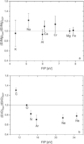
Reames (2019) reviews element abundances measured in solar energetic particles (SEPs). Large (gradual) SEP events show an abundance pattern similar to that of the SW, with low-FIP element/O ratios being enhanced by factors of 2–3 relative to photospheric abundances. SEP abundances given by Reames (2019) are compared with the values for bulk SW Genesis targets in Figure 5, where we use Mg and O as reference elements for the low-FIP (upper panel) and high-FIP (lower panel) elements, respectively. The agreement between SEP and Genesis-derived SW values is remarkably good for all low-FIP elements shown. A similarly good agreement had also been noted by Reames (2019) between SEPs and in situ derived SW abundances (Bochsler 2009), indicating a common lack of fractionation among low-FIP elements relative to the photosphere in the SW and in the higher-energy gradual SEPs. Particularly remarkable is the close agreement in Mg and Fe, which have similar FIPs.
Figure 5. Ratios of elemental abundances in Genesis bulk SW targets and solar energetic particles (SEPs). For low-FIP elements (a) Mg is used for normalization, high-FIP elements (b) are normalized to O. SEP data are from Reames (2019). Total errors (Table 1) used for Genesis data.
Download figure:
Standard image High-resolution image
The high-FIP region (Figure 5(b)) shows less good agreement between SEP and SW abundances. Most remarkably, C is enhanced in the SW by ∼30% relative to O in SEPs, while N—as well as Ar, Ne, and He—are depleted by 20%–30% in the SW relative to SEPs. A similarly high C/O ratio in the (slow) in situ SW relative to the SEP ratio was also observed by Reames (2019), who also noted even somewhat larger differences for S and P, two elements with a similar FIP to C. He pointed out that this indicates that the SEPs are not just accelerated SW but are an independent sample of the solar corona, and noted that the transition from "low FIP" to "high FIP" occurs at a lower value for SEPs than for the slow SW. The Genesis C abundance confirms this observation also for the bulk SW.
Pilleri et al. (2015) report mean abundance ratios (element/Mg) for eight elements measured by the Solar Wind Ion Composition Spectrometer (SWICS) on the Advanced Composition Explorer (ACE) during the same time window as the Genesis collection. In the upper part of Table 3, these ratios are compared with the data of this work for the five element pairs for which bulk SW data are available in both studies. For regime data, only Ne/Mg and He/Mg are available in both studies. In the lower part of the table, we report these ratios normalized to the respective bulk SW values. All five elemental abundance ratios from both studies agree within their formal uncertainties; for O/Mg and Ne/Mg, the agreement is actually very satisfying.
Table 3. Comparison of Elemental Abundance Ratios in ACE and Genesis
| Bulk SW | ACEa | ±b | Genesis | ± | ||
|---|---|---|---|---|---|---|
| Fe/Mg | 0.98 | 0.20 | 0.746 | 0.039 | ||
| C/Mg | 4.39 | 0.88 | 3.71 | 0.25 | ||
| O/Mg | 6.64 | 1.00 | 6.76 | 0.74 | ||
| Ne/Mg | 0.749 | 0.15 | 0.786 | 0.033 | ||
| He/Mg | 600 | 120 | 479 | 20 | ||
| Regimes/Bulk SW | Slow SW/Bulk SW | Fast SW/Bulk SW | CME/Bulk SW | |||
| ACEa | Genesis | ACEa | Genesis | ACEa | Genesis | |
| Ne/Mg | 0.91 | 0.94 | 1.06 | 1.17 | 1.06 | 1.08 |
| He/Mg | 1 | 0.91 | 1.07 | 1.12 | 0.89 | 1.16 |
Notes.
aACE data from ref. (1) measured by the SWICS instrument during time intervals corresponding to the respective collection periods of the Genesis bulk or regime targets. Errors for Genesis data are total errors from Table 1. bInstrumental uncertainties as reported in reference (1).Reference. (1) Pilleri et al. (2015).
Download table as: ASCIITypeset image
5. Conclusions
This paper presents data on elemental abundances in the SW for elements with a wide range in FIPs obtained by laboratory analyses on Genesis targets. Such data are of higher precision than can be reached by in situ observations and can be used to support studies of SW fractionation processes and possibly solar abundances of key elements more quantitatively than measurements obtained by space-borne instruments. All elements discussed here (C, N, O, Na, Mg, Al, Ca, Cr, H, K, Fe, and the noble gases) are also of great interest in planetary sciences. In some cases, the data presented here approach the accuracy required to test the extent to which elemental abundances of CI chondrites approach solar abundances. The Genesis data are consistent with the view that CI data represent the solar abundances of the low-FIP elements studied here as well as spectroscopically obtained values. Intermediate- to high-FIP elements between 10 and 16 eV (C, N, O, H, Kr, Xe, Ar) display a well-defined trend of increasing SW abundances with decreasing FIP if normalized to 3D-model-derived solar values. In particular, Kr and Xe, whose solar abundances are independently known and whose SW abundances are anchored to H via the well-known abundances of He in the outer convective zone of the Sun as well as in the SW, speak in favor of the 3D-model values (Asplund et al. 2009). Where Genesis data are available for the SW regimes, the fast regime is always less fractionated than the slow and CME SW, as expected, although the differences are modest. For low-FIP elements the interregime variations are precisely measured (Table 2), the fast–slow SW differences are less than 3%. Abundances of low-FIP elements measured in gradual SEP events (Reames 2019) agree well with SW abundances obtained here, whereas the high C/O ratio in the SW relative to the SEP value is consistent with the suggestion by Reames (2019) that the transition from "low-FIP" to "high-FIP" elements occurs at a lower range of ionization energies for SEPs than for the SW.
We appreciate the expertise and cooperation of the curatorial team at NASA Johnson Space Center in cleaning the Genesis collector fragments. D. Ledu, F. Fortuna (CSNSM Orsay), E. Briand, and J.-J. Ganem (Universités Pierre et Marie Curie and Namur) are thanked for standard implantations and nuclear reaction analyses. We appreciate discussions with P. Bochsler and comments and suggestions by the reviewer. The UCLA ion microprobe facility is partially supported by a grant from the NSF Instrumentation and Facilities program. V.S.H. thanks NASA for financial support. This work was supported by grants from the NASA Laboratory Analysis of Returned Samples (LARS) program (NASA LARS 80NSSC17K0025 to D.S.B. and A.J.G.J. R.W. acknowledges the hospitality of Caltech's Division of Geological and Planetary Sciences during his stay in Pasadena.
Appendix
A.1. Basic Analytical Procedures
Table 4 shows the details of each backside SIMS analysis and each individual fluence. Table 5 gives additional details. Artificial ion implants into Si served as reference. One minor isotope of the element of interest (except for Cr and the monoisotopic elements Al and Na) with approximately known nominal fluences was implanted. Profiles of the reference implants, conventionally sputtered from the front side, were routinely measured prior to and after each SW profile for the positive ions (Na, Mg, Al, Ca, and Cr) in a standard-sample bracketing mode, or several times per day for the negative ions (C, N, and O). The depth of raster pits in the reference implants was measured by a MicroXam Surface Mapping Microscope and/or a Zygo optical surface profiler (Heber et al. 2014a).
Table 4. Fluences Measured in Each Individual Backside SIMS Analysis
| Analysis# and Session Date | Isotope | Regime | Fluencea (ions cm−2) | Error, 1σ (ions cm−2) | Error Includes |
|---|---|---|---|---|---|
| 1 (10/2010) | 16O | bulk | 1.04E13 | 1.39E11 | RSF, S |
| 2 (10/2010) | 16O | bulk | 1.14E13 | 1.53E11 | RSF, S |
| average 1 and 2 | 1.09E13 | 7.12E11 | stdev. of 2 analyses | ||
| 3 (06/2012) | 16O | bulk | 1.20E13 | 2.00E11 | RSF, S |
| 4 (06/2012 | 16O | bulk | 1.22E13 | 2.03E11 | RSF,S |
| 5 (06/2012) | 16O | bulk | 1.34E13 | 2.23E11 | RSF, S |
| average 3-5 | 1.26E13 | 7.5E11 | stdev. of 3 analyses | ||
| average 16O bulk | 1.17E13b | 1.25E12 | stdev. 2 session av., RSF, S + 2.5% ref. calibrationb | ||
| 7 (10/2010) | 12C | bulk | 6.86E12 | 1.21E10 | RSF, S |
| 8 (10/2010) | 12C | bulk | 6.14E12 | 1.08E10 | RSF, S |
| 9 (10/2010) | 12C | bulk | 6.17E12 | 1.28E10 | RSF, S |
| 10 (10/2010) | 12C | bulk | 6.46E12 | 1.34E10 | RSF, S |
| 11 (10/2010) | 12C | bulk | 6.37E12 | 1.33E10 | RSF, S |
| 12 (10/2010) | 12C | bulk | 5.23E12 | 6.68E10 | RSF, S |
| 13(10/2010) | 12C | bulk | 5.57E12 | 1.16E10 | RSF, S |
| average 7-13 | 6.12E12 | 5.50E11 | stdev. of 7 analyses | ||
| 14 (06/2012) | 12C | bulk | 6.69E12 | 9.24E10 | RSF, S |
| 15 (06/2012) | 12C | bulk | 6.42E12 | 6.57E9 | RSF, S |
| average 14,15 | 6.56E12 | 1.91E11 | stdev. of 2 analyses | ||
| average 12C bulk | 6.34E12 | 3.61E11 | stdev. 2 session av., RSF, S + 2.8% ref. calibrationb | ||
| 16 (10/2010) | 14N | bulk | 1.25E12 | 3.31E10 | RSF, S |
| 17 (10/2010) | 14N | bulk | 1.55E12 | 4.11E10 | discardedc |
| 18 (10/2010) | 14N | bulk | 1.24E12 | 3.27E10 | RSF, S |
| average 16,18 | 1.24E12 | 9.23E9 | stdev. of #16 and 18 | ||
| 19 (06/2012) | 14N | bulk | 1.23E12 | 1.06E10 | RSF, S |
| 20 (06/2012) | 14N | bulk | 1.21E12 | 1.09E10 | RSF, S |
| 21(06/2012) | 14N | bulk | 1.21E12 | 1.16E10 | RSF, S |
| 22 (06/2012) | 14N | bulk | 1.21E12 | 1.10E10 | RSF, S |
| average 19-22 | 1.22E12 | 1.18E10 | stdev. of 4 analyses | ||
| average 14N bulk | 1.23E12 | 1.26E11 | stdev. 2 session av., RSF, S + 10% (missing ref. calib.) | ||
| 23 (02/2013) | 27Al | bulk | 1.40E11 | 3.94E9 | RSF, S |
| 24 (02/2013) | 27Al | bulk | 1.41E11 | 9.90E9 | RSF, S |
| 25 (04/2013) | 27Al | bulk | 1.43E11 | 3.66E9 | RSF, S |
| 26 (04/2013) | 27Al | bulk | 1.46E11 | 3.18E9 | RSF, S |
| average 27Al bulkd | 1.42E11 | 1.52E10 | stdev. 4 analyses, RSF, S + 10% (missing ref. calib.) | ||
| 27 (02/2013) | 27Al | fast | 3.71E10 | 1.09E9 | RSF, S |
| 28 (02/2013) | 27Al | fast | 3.70E10 | 1.09E9 | RSF, S |
| 29 (04/2013) | 27Al | fast | 3.65E10 | 7.70E8 | RSF, S |
| average27Al fastd | 3.69E10 | 9.83E8 | stdev. of 3 analyses, RSF, S | ||
| 30 (02/2013) | 27Al | CME | 3.62E10 | 1.02E9 | RSF, S |
| 31 (02/2013) | 27Al | CME | 3.85E10 | 1.08E9 | RSF, S |
| 32 (04/2013) | 27Al | CME | 3.81E10 | 6.93E8 | RSF, S |
| average 27Al CMEd | 3.80E10 | 1.49E9 | stdev. of 3 analyses, RSF, S | ||
| 33 (02/2013) | 27Al | slow | 5.47E10 | 1.54E9 | RSF, S |
| 34 (02/2013) | 27Al | slow | 5.48E10 | 2.00E9 | RSF, S |
| 35 (04/2013) | 27Al | slow | 5.83E10 | 8.60E8 | RSF, S |
| average 27Al slowd | 5.54E10 | 2.43E9 | stdev. of 3 analyses, RSF, S | ||
| 36 (02/2013) | 24Mg | bulk | 1.39E12 | 1.91E10 | RSF, S |
| 37 (02/2013) | 24Mg | bulk | 1.35E12 | 1.44E10 | RSF, S |
| average 24Mg bulkd | 1.37E12 | 4.89E10 | stdev. of 2 analyses, RSF, S + 2.8% ref. calibratione | ||
| 38 (02/2013) | 24Mg | fast | 3.76E11 | 5.10E9 | RSF, S |
| 39 (02/2013) | 24Mg | fast | 3.86E11 | 5.01E9 | RSF, S |
| average 24Mg fastd | 3.81E11 | 8.65E9 | stdev. of 2 analyses, RSF, S | ||
| 40 (02/2013) | 24Mg | CME | 3.64E11 | 3.75E9 | RSF, S |
| 41 (02/2013) | 24Mg | CME | 3.57E11 | 3.81E9 | RSF, S |
| 42 (02/2013) | 24Mg | CME | 3.56E11 | 3.80E9 | RSF, S |
| average 24Mg CMEd | 3.60E11 | 5.71E9 | stdev. of 3 analyses, RSF, S | ||
| 43 (02/2013) | 24Mg | slow | 5.75E11 | 7.92E9 | RSF, S |
| 44 (02/2013) | 24Mg | slow | 5.63E11 | 5.35E9 | RSF, S |
| average 24Mg slowd | 5.68E11 | 1.08E10 | stdev. of 2 analyses, RSF, S | ||
| 45 (02/2013) | 23Na | bulk | 9.76E10 | 1.57E9 | RSF, S |
| 46 (02/2013) | 23Na | bulk | 1.02E11 | 1.98E9 | RSF, S |
| average 23Na bulkd | 1.00E11 | 1.07E10 | stdev. 2 analyses, RSF, S + 10% (missing ref. calib.) | ||
| 47 (02/2013) | 23Na | fast | 2.82E10 | 5.96E8 | RSF, S |
| 48 (02/2013) | 23Na | fast | 2.65E10 | 5.50E8 | RSF, S |
| average 23Na fastd | 2.73E10 | 1.34E9 | stdev. of 2 analyses, RSF, S | ||
| 49 (02/2013) | 23Na | CME | 2.70E10 | 5.19E8 | RSF, S |
| 50 (02/2013) | 23Na | CME | 2.63E10 | 5.10E8 | RSF, S |
| 51 (02/2013) | 23Na | CME | 2.60E10 | 5.04E8 | RSF, S |
| average 23Na CMEd | 2.64E10 | 7.40E8 | stdev. of 3 analyses, RSF, S | ||
| 52 (02/2013) | 23Na | slow | 4.21E10 | 7.90E8 | RSF, S |
| 53 (02/2013) | 23Na | slow | 4.25E10 | 6.82E8 | RSF, S |
| average 23Na slowd | 4.21E10 | 7.88E8 | stdev. of 2 analyses, RSF, S | ||
| 54 (04/2013) | 40Ca | bulk | 1.11E11 | 1.88E9 | RSF, S |
| 55 (04/2013) | 40Ca | bulk | 1.16E11 | 7.38E8 | RSF, S |
| average 40Ca bulkd | 1.13E11 | 5.99E9 | stdev. of 2 analyses, RSF, S + 4.1% ref. calibratione | ||
| 56 (04/2013) | 40Ca | fast | 3.09E10 | 5.11E8 | RSF, S |
| 57 (04/2013) | 40Ca | CME | 3.21E10 | 2.03E8 | RSF, S |
| 58 (04/2013) | 40Ca | slow | 4.62E10 | 3.46E8 | RSF, S |
| 59 (04/2013) | 40Ca | slow | 4.67E10 | 4.48E8 | RSF, S |
| average 40Ca slowd | 4.65E10 | 5.29E8 | stdev. of 2 analyses, RSF, S | ||
| 60 (04/2013) | 52Cr | bulk | 1.95E10 | 3.06E8 | RSF, S |
| 61 (04/2013) | 52Cr | bulk | 1.95E10 | 5.62E8 | RSF, S |
| average 52Cr bulk5 | 1.95E10 | 9.40E8 | stdev. of 2 analyses, RSF, S + 4.3% ref. calibratione | ||
Notes. Analysis number in column 1 used to identify analysis in Table 5.
aFluences (for isotopes measured, not total elements) backscatter-corrected according to prevailing solar wind conditions during collection. Uncertainties include the standard deviations of RSF and S (see Appendix A.2) measured in reference implants for the elements measured as positive ions. For C, N, and O, we include the standard deviation of RSF and S over a day. bUncertainty of reference calibration calculated from Orsay implant data (Heber et al. 2014a). cMeasurement interrupted near concentration peak. Onset of breakthrough difficult to assess. dAverage fluences for positive ion profiles weighted based on completeness of data coverage. eUncertainties of reference calibrations include standard deviations of n analyses of standard glasses (Table 6), concentration uncertainties of standard elements in the glasses, and uncertainties of pit depths measured with a profilometerTable 5. Details of Individual Backside SIMS Analyses
| Analysis # | NASA Sample Code | DE (nm) | FE (%) | Method to Account for Missing Data | Reference Implant | Profile Displayed in |
|---|---|---|---|---|---|---|
| 1 and 2 (16O) | 30767 | 30/24 | 21/17 | Mg Analysis #39, 2nd Order Polynomial | Orsay Implant K09-07_18O15N During Measurement With Fluence Adjusted) | |
| 3–5 (16O) | 30767 | 22/24/22 | 15/17/15 | Mg analysis #39, 2nd order polynomial | Orsay K09-07_18O15N during measurement with fluence adjusted | Figure 1(b) and ref. (1): Figures 9(a) and 10(f) |
| 7–11 (12C) | 60757 | 25/17/23/25/22 | 18/11/16/18/15 | Mg analysis #39, 2nd order polynomial | Orsay implant (LANL 5_05_13C during measurement with fluence adjusted) | Figure 1(b) |
| 12–13 (12C) | 30767 | 26/31 | 20/24 | Mg analysis #39, 2nd order polynomial | Orsay implant (LANL 5_05_13C during measurement with fluence adjusted) | |
| 14–15 (12C) | 60968 | 23/22 | 17/15 | Mg analysis #39, 2nd order polynomial | Orsay implant (LANL 5_05_13C during measurement with fluence adjusted) | ref. (1): Figure 9(c) |
| 16–18 (14N) | 60757 | 13/21/15 | 6/15/8 | K 04_2013_AlCa | EAG 4257 (K09-07_18O15N during measurement with fluence adjusted) | |
| 19–22 (14N) | 60968 | 14/12/14/16 | 7/5/7/8 | Mg analysis #39, 2nd order polynomial | EAG 4257 (K09-07_18O15N during measurement with fluence adjusted) | Figure 1(c); ref. (1): Figure 9(b) |
| 23 (27Al) bulk | 60514 | 12 | 5 | 2nd order polynomial | K 04_2013_AlCa (K 08-08_Al used during measurement with fluence adjusted) | |
| 24 (27Al) bulk | 60514 | 11 | 7 | Asym2sig (Origin®), 2nd order polynomial | K 04_2013_AlCa (K 08-08_Al used during measurement with fluence adjusted) | |
| 25 (27Al) bulk | 30768 | 15 | 8 | Asym2sig (Origin®), 2nd order polynomial | K 04_2013_AlCa | |
| 26 (27Al) bulk | Mg analysis #39, 2nd order polynomial | K 04_2013_AlCa | ||||
| 27–29 (27Al) fast | 60796 | 7.3/2.8/ 6.5 | 0.6/0.1/0.5 | 2nd order polynomial | K 04_2013_AlCa (K 08-08_Al used during measurement with fluence adjusted) | |
| 30 (27Al) CME | 41126 | 18 | 10 | Al analysis #31, 2nd order polynomial | K 04_2013_AlCa (K 08-08_Al used during measurement with fluence adjusted) | |
| 31 (27Al) CME | 41126 | 3.4 | 0.6 | 2nd order polynomial | K 04_2013_AlCa (K 08-08_Al used during measurement with fluence adjusted) | |
| 32 (27Al) CME | 41133 | 3.9 | 0.7 | 2nd order polynomial | K 04_2013_AlCa | ref. (1): Figure 10(c) |
| 33–34 (27Al) slow | 60833 | 1.4/4.5 | 0.2/2 | 2nd order polynomial | K 04_2013_AlCa (K 08-08_Al used during measurement with fluence adjusted) | |
| 35 (27Al) slow | 60449 | 8.7 | 6 | Al analysis #33, 2nd order polynomial | K 04_2013_AlCa | |
| 36–37 (24Mg) bulk | 60514 | 4.8/3.2 | 1.1/0.5 | 2nd order polynomial | K 02_2010 25Mg (K 02_2013 Na25Mg used during measurement with fluence adjusted) | ref. (1): Figure 10(a) and 7a |
| 38–39 (24Mg) fast | 60796 | 1.6/4.5 | 0.0/0.3 | 2nd order polynomial | K 02_2010 25Mg (K 02_2013 Na25Mg used during measurement with fluence adjusted) | Figure 1(e) |
| 40–41 (24Mg) CME | 41126 | 5.2/3.9 | 1.2/0.9 | 2nd order polynomial | K 02_2010 25Mg (K 02_2013 Na25Mg used during measurement with fluence adjusted) | Figure 1(d) |
| 42 (24Mg) CME | 41126 | Mg (41126, analysis 41), 2nd order polynomial | K 02_2010 25Mg (K 02_2013 Na25Mg used during measurement with fluence adjusted) | |||
| 43–44 (24Mg) slow | 60833 | 11.1/2.4 | 6.9/0.5 | 2nd order polynomial | K 02_2010 25Mg (K 02_2013 Na25Mg used during measurement with fluence adjusted) | ref. (1): Figure 9(e) |
| 45–46 (23Na) bulk | 60514 | 12.8/11.0 | 6/9 | 2nd order polynomial, end of profile set by Mg of same measurement | K 02_2013 Na25Mg | ref. (1): Figure 10(d) |
| 47–48 (23Na) fast | 60796 | 12.9/9.6 | 2/1.1 | 2nd order polynomial, end of profile set by Mg of same measurement | K 02_2013 Na25Mg | Figure 1(e) |
| 49–50 (23Na) CME | 41126 | 22.9/9.8 | 16/4 | 2nd order polynomial, end of profile set by Mg of same measurement | K 02_2013 Na25Mg | |
| 51 (23Na) slow | 41126 | 31.7 | 14 | Mg of same measurement, 2nd order polynomial | K 02_2013 Na25Mg | |
| 52–53 (23Na) slow | 60833 | 9.6/28.5 | 5/33 | 2nd order polynomial, end of profile set by Mg of same measurement | K 02_2013 Na25Mg | |
| 54–55 (40Ca) bulk | 60998 | 3.3/12.2 | 0.7/5 | 2nd order polynomial | K 04_2013_AlCa | Figure 1(g); ref. (1): Figure 9(f) |
| 56 (40Ca) fast | 60796 | 7.0 | 0.9 | 2nd order polynomial | K 04_2013_AlCa | |
| 57 (40Ca) CME | 41133 | 4.3 | 0.9 | 2nd order polynomial | K 04_2013_AlCa | |
| 58–59 (40Ca) slow | 60449 | 15.1/10.1 | 16/9 | Asym2sig (Origin® fit) of Mg analysis #44, 2nd order polynomial | K 04_2013_AlCa | ref. (1): Figure 10(e) |
| 60–61 (52Cr) bulk | 2nd order polynomial | CEI 62Ni, 52Cr 01/2013 and L52 (with fluence adjusted) | Figure 1(h); ref. (1): Figure 10(b) |
Notes. Analysis # in column 1 refers to column 1 in Table 4.
aDE = Extrapolated distance to target surface of last measured point before breakthrough. bFE = Extrapolated fluence of unrecovered near-surface portion as fraction of total fluence FT.Reference. (1) Heber et al. (2014a).
All analyses of reference and SW profiles were done under identical conditions in each given session. The standard-sample bracketing technique allowed us to reduce the uncertainties of calibration factors due to instrumental variations, especially important for the regime samples that were expected to show abundance differences of a few percent at best if low-FIP elements are unfractionated relative to each other.
A.2. Data Reduction
Measured signals of the isotope of interest were corrected for the effective dead time of the counting system and for background contributions. No correction was made for the instrumental mass fractionation between the isotopes measured in the reference implant and the sample, respectively, as such effects are small compared to the overall uncertainty of the SW fluence determinations.
From the reference implants sputter rates (S) and SW fluences (Fi) were obtained according to Equations (1) and (2):

with x being the measured pit depth and t the total sputter time of a profile. Sputter rates obtained for the reference implants were used for the sample backside profiles measured prior to and afterwards. A sensitivity factor, RSF, is used to relate implant standard secondary ion intensity, normalized to the matrix element Si, to standard implant fluence (Heber et al. 2014a; Burnett et al. 2015).
The unknown SW fluence (Fi) of an isotope of interest is calculated from its depth profile according to Equation (2):

with ni and nSi being the ion intensities in counts per second of the isotope of interest and the matrix element Si, respectively. Equation (2) is also used with a known implant standard fluence to determine RSF.
For species implanted to depths as shallow as SW ions, measured backside depth profiles never reach the SW surface. Even low-energy primary ions of 5–7 keV as used here penetrate by about 5–10 nm into the target. This penetration causes epoxy and other contaminants from the original surface to be backward-gardened and eventually dominate the secondary ion signal. At this point, a measurement had to be stopped, and an extrapolation of the profile to the SW surface is required to determine an extrapolated surface correction (FE) to the measured profile.
Figure 1 in the main text shows, for each element, one measured backside profile; further examples (listed in Table 5) are given by Heber et al. (2014a). The most complete profiles were obtained for the positive ions, with the extrapolated fluence (FE) in the unrecovered near-surface portion on average contributing only ∼5% to the total fluence (FT). The most complete measured profiles were obtained for Mg (FE = 1.1% of FT). The distance between the last measured "good" data point to the extrapolated original surface (DE) was on average 10 nm. The negative ion profiles (C, N, O) are characterized by earlier breakthroughs, at around the depth of the maximum SW concentration. This is the result of the high abundances of these elements on surfaces (e.g., the uppermost 2 nm of metallic Si consist of a native SiO2 layer) and because these elements are the main constituents of epoxies.
The near-surface portions of the depth profiles were extrapolated as follows (see Heber et al. 2014a for more details): the nearly complete Mg profiles indicate that the measured data between the peak region and the original collector surface are well described by a quadratic polynomial. Such polynomials were therefore fitted to all profiles whose measured data extended from the peak to at least one-third of the distance toward the collector surface. This included 30 of the 39 profiles obtained with positive ions (Na, Mg, Al, Ca, and Cr). For all Na profiles, the distance to the collector surface was set equal to that of the concomitantly measured Mg profile, as Na always broke through earlier than Mg by a few nanometers. Data coverage on the collector surface side of the profile peaks was insufficient for this approach for nine profiles obtained with positive ions and all negative ion profiles. In these cases, we adopted the shape of a more complete profile of the same element (or sometimes of Mg) obtained in another analysis or of Mg from the same SW regime (main text; Figures 1(a)–(c)). This approach is justified as our data and simulations by the SRIM code (Stopping and Range of Ions in Matter; Ziegler et al. 2010) show that depth distributions and peak depths of different elements implanted with the same energy distribution are similar to each other. FE (given as the percent of FT) and DE values as well as the applied extrapolation method are given in Table 5.
Total fluences (FT) were obtained by adding the extrapolated fluence FE integrated over the fit polynomial between breakthrough and collector surface to the measured fluence (integrated over the measured data). Finally, small corrections to the fluences were made for backscatter loss upon SW implantation into the Si target. The backscatter correction factors were obtained by SRIM using the SW speed distributions at the time of the Genesis collection period (Reisenfeld et al. 2013).
A.3. Absolute Calibration of the Reference Implant Fluences
SW fluences were calibrated against reference implants with nominal fluences on the order of 1013 ions cm−2 for positive ions and (0.5–1) × 1015 ions cm−2 for negative ions. These nominal fluences have uncertainties of ∼10%, sometimes more, and require independent calibration. Heber et al. (2014a) absolutely calibrated some reference implants. Briefly, the C and O reference implant fluences were cross-calibrated with independent implantations at the Centre de Sciences Nucléaires et de Sciences de la Matière (CSNSM) Orsay (France) and the accuracy of the 18O fluence was further cross-checked by nuclear reaction analysis at the Université de Namur (Belgium). For N, we relied on one 15N implant that also contained implanted 18O and 13C with fluences in agreement with those determined in Orsay to within 4% and 2%, respectively, and added an uncertainty of 10% to account for the missing absolute calibration. The Mg, Cr, and Ca reference implants were calibrated using standard glasses with known concentration of these elements. Glasses and Si wafers that were used as reference during the SW analysis were simultaneously implanted (Burnett et al. 2015). Absolutely calibrated fluences of C and O in the Orsay implants and the resulting differences from our reference implants are given in Table 4 in Heber et al. (2014a), while Table 6 here gives the updated results for Mg, Ca, and Cr.
Table 6. Calibration of Reference Implants for Mg, Ca, Cr: Glass Parameters and the Calibrated Implant Fluence
| Standard Glass Parameters | Implant | ||||||||
|---|---|---|---|---|---|---|---|---|---|
| Type | Density (g cm−3) | Concentration (ppm) | Implanted Isotope | Implant Identification Number | Nominal Fluence (1013 cm−2) | Mean Calibrated fluence (1013 cm−2) | Number (n) of Analyses | Calibrated to Nominal Fluence (% Deviation) | |
| Mg | NIST 617 | 2.51 | 26.5 ± 0.4a | 25Mg | K SRINI 4 02/2010 | 3.0 | 2.73 ± 0.08 | 7 | −8.9 |
| Ca | SRM 93a | 2.26 | 86.8 ± 1.4 | 42Ca | K Al,42Ca 04/2013 | 1.0 | 1.18 ± 0.05 | 3 | 18.24 |
| Cr | NIST 612 | 2.51 | 36.26 ± 1.16b | 52Cr | CEI 62Ni,52Cr 01/2013 | 4.0 | 4.16 ± 0.18 | 6 | 4.10 |
Notes.
aBurnett et al. (2015). bJochum et al. (2011).Download table as: ASCIITypeset image
The Na implant calibration is from Rieck (2015; see also Rieck et al. 2016). An absolute calibration was obtained by Rutherford backscattering analysis on a nominal 1 × 1016 cm−2 (1E16) Na implant into diamond-like C (DLC) giving a calibrated fluence of 1.136 ± 0.010 × 1016 cm−2 (error is 1σ mean of 10 spectra). Si samples coimplanted with the DLC have the same fluence (Burnett et al. 2015). The K Al 42Ca 2013 nominal 1 × 10¹³ implant used as a standard for SW Na analyses cannot be intercalibrated directly with the 1E16 implant; our SIMS dynamic range is insufficient because of our inability to do accurate dead-time corrections with a rastered beam. Consequently, an intermediate ("Stevie") nominal 1 × 10¹⁴ implant was calibrated relative to the 1E16 implant. Separately, the 2013 Na implant was calibrated relative to Stevie. The fluence of the 2013 Na implant is 1.230 ± 0.66 × 1013 cm−2. This is slightly revised from the 1.28 value given in Rieck (2015).
Using the approach of Burnett et al. (2015), a nominal 1 × 1013 cm−2 42Ca implant Si standard was coimplanted with a sample of NIST 93a standard glass as the absolute reference material. The Ca concentration of the 93a glass sample was measured by an electron microprobe (emp) at Caltech to be 86.8 ± 1.4 ppm; relative to this, SIMS analyses of the 42Ca-implanted 93a glass sample yielded a 42Ca implant fluence of 1.18 × 1013 cm−2. Allowing for the error in the emp analysis, the 42Ca implant fluence is 1.18 ± 0.05 × 1013 cm−2. At this relatively low Ca concentration, the emp Ca analyses were not routine; variable emp Ca concentrations were measured adjacent to SIMS pits, which showed a uniform 40Ca/28Si counting rate ratio; however, 86.8 ppm within error defined a baseline value for around two-thirds of the analyses and the rest were higher. Detailed emp analyses ruled out significant effects from Na or B migration; the high values very likely reflect Ca surface contamination. Simultaneous SIMS/emp analyses show similar contamination effects for Al in olivine at ≈100 ppm levels (Paque et al. 2020). The calibrated 42Ca implant Si sample coimplanted with 93a was used as a standard for SW analyses.
A.4. Noble Gas Fluences in the Solar Wind Derived from Genesis Targets
The noble gas fluences shown in Table 1 in the main text are based on the values published by Heber et al. (2009, 2012) for He, Ne, and Ar and by Vogel et al. (2011, 2019) for Kr and Xe, with values for major isotopes of each element given in these publications being recalculated to elemental fluences using SW isotopic ratios measured in Genesis targets by Heber et al. (2009, 2012) for He, Ne, and Ar and by Meshik et al. (2014, 2020) for Kr and Xe (for the latter two elements, bulk SW isotopic composition was assumed also for the regimes). In detail, for He, Ne, and Ar, we adopt values from the DOS targets analyzed by Heber et al. (2009, 2012) and fully published (including the DOS regime) in Table 2 in Vogel et al. (2019). For bulk SW, we adopt the data measured in the bulk SW targets (as opposed to calculated values based on exposure-weighted regime targets. The Kr and Xe fluences in Table 1 are based on the CZ-Si target analyses given by Vogel et al. (2019), again for bulk SW we rely on the data from the bulk SW Si target. As the 36Ar fluences measured in the different Si samples differ by up to 5% from the preferred DOS values, we adjusted the Kr and Xe fluences reported by Vogel et al. (2019) to account for these differences, i.e., we adopt the mean flux ratios Kr/Ar and Xe/Ar bulk SW and each regime, respectively.
A.5. Solar Elemental Abundances and Solar-normalized Fluence Ratios
Table 7 shows solar elemental abundances adopted here. Table 8 lists solar-normalized fluence ratios in SW regimes shown in Figure 2.
Table 7. Solar Abundances Used in This Work
| Element | FIP (eV) | Abundance (dex) | ± | Element/Mg | ± a | References |
|---|---|---|---|---|---|---|
| C | 11.26 | 8.43 | 0.05 | 6.76 | 0.81 | 1 |
| N | 14.53 | 7.83 | 0.05 | 1.70 | 0.24 | 1 |
| O | 13.61 | 8.69 | 0.05 | 12.3 | 1.5 | 1 |
| Na | 5.14 | 6.21 | 0.04 | 0.0417 | 0.0040 | 2 |
| Mg | 7.65 | 7.59 | 0.04 | = 1 | 2 | |
| Al | 5.99 | 6.43 | 0.04 | 0.0692 | 0.0036 | 2 |
| K | 4.34 | 5.04 | 0.05 | 0.0028 | 0.0003 | 2 |
| Ca | 6.11 | 6.32 | 0.03 | 0.0537 | 0.0038 | 2 |
| Cr | 6.77 | 5.62 | 0.04 | 0.0107 | 0.0010 | 3 |
| Fe | 7.87 | 7.47 | 0.04 | 0.759 | 0.072 | 3 |
| H | 13.6 | 12 | 25700 | 3080 | ||
| Heb | 24.58 | 10.92 | 0.01 | 2140 | 105 | 4 |
| Nec | 21.56 | 8.05 | 0.02 | 2.87 | 0.12 | 5 |
| Arc | 15.75 | 6.36 | 0.04 | 5.87E-2 | 0.50E-2 | 5 |
| Krd | 13.99 | 3.25 | 4.56E-5 | 0.33E-5 | ||
| Xee | 12.13 | 2.26 | 4.66E-6 | 0.29E-7 |
Notes.
aNot including the Mg uncertainty. bHelioseismology. cNe/He and Ar/He versus H/He in the Genesis regimes extrapolated to solar H/He according to Huss et al. (2020), with slightly updated Ne and Ar values obtained with data in Table 1 of this work. dInterpolated from CI chondrite abundances of neighboring elements. eFrom s-process σn trends.References. (1) Asplund et al. (2009). (2) Scott et al. (2015b). (3) Scott et al. (2015a). (4) Basu & Antia (2008) (5) Huss et al. (2020).
Download table as: ASCIITypeset image
Table 8. Fluence Ratios (Element/Mg) in Solar Wind Regimes Normalized to Solar Values: (E/Mg)SW/(E/Mg)sol
| Bulk SW | ± | Slow | ± | Fast | ± | CME | ± | |
|---|---|---|---|---|---|---|---|---|
| C | 0.536 | 0.074 | ||||||
| N | 0.409 | 0.073 | ||||||
| O | 0.537 | 0.087 | ||||||
| Na | 1.706 | 0.205 | 1.728 | 0.033 | 1.672 | 0.085 | 1.710 | 0.047 |
| Mg | 1.000 | 0.107 | 1.000 | 0.019 | 1.000 | 0.023 | 1.000 | 0.015 |
| Al | 1.186 | 0.174 | 1.114 | 0.048 | 1.107 | 0.030 | 1.205 | 0.048 |
| Ca | 1.259 | 0.118 | 1.243 | 0.013 | 1.232 | 0.019 | 1.352 | 0.008 |
| Cr | 1.252 | 0.140 | ||||||
| H | 0.367 | 0.059 | 0.338 | 0.012 | 0.445 | 0.005 | 0.352 | 0.013 |
| He | 0.227 | 0.014 | 0.208 | 0.001 | 0.255 | 0.001 | 0.263 | 0.001 |
| Ne | 0.266 | 0.036 | 0.249 | 0.001 | 0.312 | 0.001 | 0.287 | 0.001 |
| Ar | 0.333 | 0.057 | 0.315 | 0.002 | 0.404 | 0.004 | 0.330 | 0.002 |
| Kr | 0.279 | 0.030 | 0.264 | 0.003 | 0.340 | 0.006 | 0.271 | 0.003 |
| Xe | 0.604 | 0.064 | 0.546 | 0.012 | 0.619 | 0.027 | 0.560 | 0.028 |
Note. Fluence ratios shown in Figure 2.
Download table as: ASCIITypeset image
A.6. Comparison of Genesis and in Situ Interregime Element Ratios
As discussed in conjunction with Figure 2(b) and Table 2 in the main text, our results show very similar element/Mg ratios among the three regimes at a very high level of precision for low-FIP elements. Here we show that this result is compatible with previous studies of SW composition. All abundance data in this section are the measured SW ratios; no data normalized to spectroscopic photospheric ratios are used. Beyond the higher precision of our data, there are other reasons why the similarity in low-FIP trends has not been recognized: (1) use of O normalization. (2) Differences (at present) among low-FIP elements for Genesis and spacecraft instrument studies.
O normalization. Discussions of SW composition require a reference element. O is the logical choice for spacecraft data, as the data are very precise. All spacecraft data papers, except Pilleri et al. (2015), normalize to O. For Genesis, O is difficult to measure, in contrast to Mg, which we have adopted as a reference element. The widely accepted qualitative interpretation of the large low–high FIP elemental fractionation in all coronal and solar particle abundance data is that it represents the lack of complete ionization for high-FIP elements, producing their depletion. Correct interpretations do not require any specific reference element; however, in terms of assessing interregime variations of low-FIP elements, data normalized to a high-FIP element (e.g., O) can be confusing. Using the most recent revised ACE-SWICS data (Pilleri et al. 2015) for the Genesis mission period, the L ("slow SW") and H ("fast SW") Mg/O ratios are 0.156 and 0.128, respectively. Because the photospheric Mg/O is 0.079, one concludes, correctly, that the H SW is less fractionated. But, the statement: "L SW is more enhanced in low-FIP elements than H SW," although numerically correct, is potentially misleading because the main fractionation is between low-FIP elements as a group and any specific high-FIP element. The cause of the (L, H) Mg/O difference is less O depletion in the H SW. This is totally semantic, but O normalization makes the very similar interregime element ratios of low-FIP elements more difficult to see. This problem does not arise in Mg-normalized data.
Element selection. Our high-precision interregime comparisons involve: Na, Ca, Al, and Mg. The most accurate ACE-SWICS data (Pilleri et al. 2015) only have Mg, Fe, and Si. The only overlap is Mg. With FIP = 8.15 eV, Si may not be a low-FIP element; nevertheless, the L and H Si/Mg ratios are very close: 1.19 and 1.21. The spectroscopic photospheric ratio is 0.81 ± 0.11 (Asplund et al. 2009), possibly not significant relative to Pilleri at 2σ. The main point is that the Si/Mg is the same in L and H SW, consistent with the conclusion from our data for other low-FIP elements. Pilleri et al. give evidence that a separate mass-dependent fractionation causes L–H differences in Fe/Mg.
Comparison with MTOF abundances. In order to deal with the complex SW charge state distribution, the mass time of flight (MTOF) mass spectrometer (Hovestadt et al. 1995; Heidrich-Meisner et al. 2016) passed velocity-selected SW ions through a thin foil such that only +1 charged ions emerged. Beautiful mass spectra were obtained, but there have been major problems in obtaining quantitative elemental abundances because a large correction is required for the fraction of incoming ions that emerge from the foil as neutrals. Progress appears to have been made (Heidrich-Meisner et al. 2016) by intercalibration with SWICS, but quantitative abundances are not yet available. A full set of MTOF abundances for the same elements as measured here is available in Table 1 of Bochsler (2009). For L and H SW, the Na/Mg, Al/Mg, and Ca/Mg ratios are the same in L and H SW, although the errors range from 25% to 75%, compared to our 2%–5%.