


Abstract
Spatial gradients of galactic cosmic-ray (GCR) fluxes are important for studying charged particle transport in the heliosphere. Little is known so far about how these gradients evolve with time. Here we present how the radial gradient (Gr) evolves between 2006 January and 2017 September using Cassini measurements of >300 MeV protons, which we combine with proton spectra obtained by advanced observatories at Earth (BESS, BESS-Polar, PAMELA, and AMS-02). All gradient calculations were performed for a nearly constant heliocentric distance of Cassini from Earth's orbit and near the ecliptic, thus revealing only how Gr changes with time. The variability patterns of Gr are well established as they rely on a single data set for ∼9.5 au and accurately cross-calibrated GCR spectra for Earth at 1 au. We show that over solar-cycle timescales, Gr is regulated by both the polarity of the solar magnetic field and the solar-cycle phase. During the negative-polarity phase (A < 0, 2006–2014), gradients are stronger and more stable with an average of Gr = 3.5 ± 0.3%/au and with evidence of a minimum around the 2009 solar minimum. The gradient peaks at ∼4%/au around the solar maximum and subsequently experiences a gradual drop to ∼2%/au in the A > 0 phase (2014–2017). Regular Gr enhancements over yearly or biennial timescales are also observed, in phase with quasi-biennial oscillations in GCR intensity. While all aforementioned results are based on Cassini measurements that are integral in energy, they are most representative for GCR protons in the low gigaelectronvolt range.
Export citation and abstract BibTeX RIS
1. Introduction
Galactic cosmic rays (GCRs) are high-energy charged particles of astrophysical origin. They comprise mostly protons, electrons, and heavier ions reaching into ultrarelativistic energies. Due to their high energies, GCRs cross the heliopause and gain access to the entire heliosphere. They are regularly detected through ground-based measurements by neutron monitors and through energetic particle detectors on board spacecraft that operate in different regions of our solar system (e.g., Heber et al. 1995; Adriani et al. 2013; Usoskin et al. 2017; Roussos et al. 2018a; Honig et al. 2019). Owing to the Voyager 1 and 2 spacecraft, GCRs have even been measured in the local interstellar medium (LISM), before their distribution is modified by interaction with the heliosphere (Krimigis et al. 2013, 2019; Stone et al. 2013, 2019; Cummings et al. 2016).
All these measurements are indicative of the different processes that GCRs undergo as a function of heliocentric distance, latitude, energy, and time from the moment they gain entry to our Local Bubble until they reach the inner heliosphere. A well-documented characteristic is the solar modulation of GCRs at a variety of timescales, including the solar rotation and the solar cycle (Reames 1999; Cane 2000; Heber et al. 2006; Adriani et al. 2013; Heber 2013). These modulations are revealing about the transport of GCRs within the heliosphere, which can be described through a variety of approximations or models (e.g., Vainio et al. 2009; Kóta 2013; Moraal 2013; Potgieter 2013; Boschini et al. 2018). A measurable index that can be contrasted against different transport model predictions is the radial intensity gradient of GCRs. This gradient is defined as

where j1 and j2 are GCR intensities at the heliocentric distances r1 and r2, respectively. This parameter is easily calculated when simultaneous measurements are available at different heliocentric distances and assuming that Gr between the two locations is constant. Intensity gradients exist also as a function of heliospheric latitude. These need to be disentangled from the radial gradients if spacecraft measurements are taken away from the ecliptic, as was done by de Simone et al. (2011), Gieseler & Heber (2016), and Vos & Potgieter (2016), who analyzed measurements by the Ulysses solar orbiter (Heber 2013) and the Payload for Antimatter Matter Exploration and Light-nuclei Astrophysics (PAMELA; Picozza et al. 2007).
Data-based calculations of Gr are available from a variety of independent studies and for different ion species and energies. Estimates of Gr for the inner heliosphere and for protons up to a few gigaelectronvolts converge to values lower than ∼5%/au (McKibben 1975; McDonald et al. 2003; de Simone et al. 2011; Gieseler & Heber 2016; Vos & Potgieter 2016; Honig et al. 2019). Many of these measurements, however, are subject to a series of uncertainties. Some of these uncertainties may be systematic, due to cross-calibration issues between measurements obtained from different techniques and instruments at various regions of the heliosphere or because radial, temporal, and latitudinal dependencies of Gr are not always straightforward to distinguish. These kind of problems make combining Gr values from independent investigations and time periods challenging, such that long-term time series of Gr cannot be constructed without ambiguity. Several examples are provided below.
Lockwood & Webber (1984) studied the period containing the transition between solar cycles 20 and 21 (1972–1982), including the polarity reversal from A > 0 to A < 0 around 1980. Combining data from Voyager 1, Pioneer 10, and the Interplanetary Monitoring Platform-8 (IMP-8), the authors did not resolve any long-term variation of Gr within 25 au from the Sun. Conversely, when a similar period was investigated using proton measurements from Pioneer 10 and Pioneer 11 (1972–1988, 1–44 au), Gr was found to experience a sinusoidal variation over the solar cycle, with values peaking around the time of the solar maximum (1979–1981; van Allen 1988). Webber & Lockwood (1991) obtained a trend similar to that found by van Allen (1988) for 1982–1990 using Pioneer 10, Voyager 1 and 2, and IMP-8 measurements (increasing Gr toward solar maxima) but different Gr values at the overlapping date range of the two studies. Webber & Lockwood (1991) argued that the differences could be attributed to the diverse conditions under which the GCR measurements were obtained, namely the different heliocentric distance and latitude ranges.
More recently, time series of Gr were calculated by Honig et al. (2019) using measurements from nearly identical radiation monitors on Earth orbiters and on the Rosetta spacecraft that reached out to 5.7 au. The authors provide evidence of a cyclic Gr variation between 2005 and 2014. Most notable are the strong variations of Gr, ranging between 1.6 and 2.1%/au in 2005 and 2014 and 3.1%/au in the years around the solar minimum (2008–2011). The peak values during the solar minimum would point to a reversed solar-cycle dependence of Gr compared to what van Allen (1988) and Webber & Lockwood (1991) found. Since estimates of Gr by Honig et al. (2019) between these periods were discrete rather than continuous, it is uncertain if the observed changes were rapid or gradual and whether there were specific correlations with well-timed events such as the solar magnetic field polarity reversal from A < 0 to A > 0 (Sun et al. 2015) between 2014 and 2015. The study even hints that in 2014 the comet 67P (target of the mission) may have influenced GCR intensities measured by Rosetta, thus explaining, at least in part, the reduced Gr for that period.
From the short review provided above, it is obvious that the long-term solar-cycle variability of Gr is far from established. Assessing this time variation, however, could offer new insights on the transport of GCRs in the heliosphere and throughout the solar cycle (Manuel et al. 2015). To address this problem, we analyze GCR measurements from the Low Energy Magnetospheric Measurement System (LEMMS) of the Cassini spacecraft in combination with observations at Earth at 1 au. The rationale for using Cassini/LEMMS measurements for this purpose is analyzed in the following section.
2. Using Cassini as a GCR Observatory
Cassini was launched in 1997 October and orbited Saturn between 2004 July and 2017 September. The capability of using LEMMS to resolve GCR time series has been demonstrated in a variety of studies (Roussos et al. 2011, 2018a, 2018c, 2019). For the present study, the advantages of using Cassini data are the following:
- 1.After 2004 and for 13 yr, Cassini was at a quasi-steady distance from 1 au, and any possible heliocentric distance dependence of Gr that we will estimate for that period is negligible.
- 2.
- 3.During its interplanetary transfer to Saturn, Cassini flew by the Earth (1999 August), with LEMMS operating for several weeks around that period (Lagg et al. 2001). These measurements can be compared with independent observations of GCR spectra at 1 au, offering data for the absolute calibration of LEMMS's GCR count rates.
- 4.A fortuitous coincidence was the launch and operation of the Balloon-Borne Experiment with a Superconducting Spectrometer (BESS) on 1999 August 29 (BESS99; Shikaze et al. 2007), a few weeks after Cassini's flyby from Earth and while the spacecraft was still near 1 au. BESS99 obtained high energy resolution GCR spectra, which can define an ideal point of reference for cross-calibrating LEMMS's GCR responses (Section 3).
- 5.Measurements by advanced energetic particle observatories like PAMELA and the Alpha Magnetic Spectrometer-2 (AMS-02; Picozza et al. 2007; Aguilar et al. 2018) provide time series of high-precision GCR differential spectra at 1 au. These spectra are available from 2006 until the end of the Cassini mission in 2017 and can be used as the reference for the application of Equation (1). Such high-quality spectra simplify cross-calibration efforts, as discussed in Section 3.
- 6.Simultaneous measurements between 2006 and 2017 at 1 and 9.5 au span one solar cycle and the polarity reversal of the solar dipole from A < 0 to A > 0 around 2013 (Sun et al. 2015).
In the following sections, we explain how we utilize all of these advantages for calculating Gr between 1 and 9.5 au and describe our findings on the gradient's long-term variability, with an emphasis on solar-cycle and yearly timescales.
3. Multipoint GCR Measurements
As explained in the introduction, application of Equation (1) requires simultaneous measurements of GCRs at two different locations. The following subsections describe the different sources of GCR data for the present study. We also introduce an analytical model that approximates the GCR proton distribution function and that provides additional context.
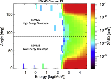
Figure 1. Response function of channel E7 as a function of proton energy and polar angle of incidence to LEMMS. Centered at 0° and 180° are the apertures of LEMMS's Low and High Energy Telescopes (LET/HET), respectively. The response from any telescope side is maximized within a cone of 30° around each aperture's bore sight. Color-coded values show the effective channel area for proton acceptance with a given combination of energy and polar angle.
Download figure:
Standard image High-resolution image3.1. GCR Measurements at 9.5 au: Cassini MIMI/LEMMS
LEMMS was a double-ended energetic charged particle telescope that belonged to Cassini's Magnetospheric Imaging Instrument (MIMI) suite (Krimigis et al. 2004). The signal of GCRs in LEMMS, which appears as low-intensity background noise in many of its 57 channels, can be easily isolated. We refer the reader to Roussos et al. (2018a, 2019) for the details on how this signal is extracted, and we focus on the data processing aspects that are most relevant or novel for the present investigation. Additional information is provided in the Appendix.
A new element compared to the past, the Cassini-based GCR studies that we cite above, is that we extended our data set back to the first switch-on of the LEMMS instrument on 1999 January 3. The main purpose was to analyze the LEMMS GCR data around the time of the Earth flyby, compare them with well-defined measurements of GCR proton spectra at 1 au (Section 3.2), and obtain an absolute GCR flux calibration for LEMMS.
Here we use data from LEMMS channel E7. Away from sources of planetary electrons and protons in Saturn's radiation belts, E7 is responding to >300 MeV protons. The signal-to-noise ratio easily exceeds 50 when few-days averaging is applied to its GCR time series. In addition, the E7 calibration settings were identical at 1 au and for the Saturn tour, while the channel shows no sensitivity to neutrons and gamma rays from Cassini's Radioisotope Thermal Generators (RTGs). At the energies of E7, protons are dominated by GCRs for periods with quiet solar wind. Solar proton fluxes become comparable or stronger only at energies below ∼10–20 MeV.
The channel's most important property is that contributions to its signal from sideways-penetrating GCR protons is the lowest compared to all LEMMS proton channels. Sideways penetrators may propagate through the body of the Cassini spacecraft before reaching LEMMS, an effect not taken into account in our channel-response function simulations. In that respect, we consider that the modeled responses of E7 (Figure 1) are the most reliable compared to other LEMMS channels. The channel's directionality and capability to reject sideways penetrators have been confirmed through measurements of the harsh environments of Earth's and Saturn's proton radiation belts (Roussos et al. 2018b). The processing steps for E7 data were the following:
- 1.We excluded time periods through Earth's and Saturn's radiation belts, as well as data for an extended period around the Cassini flyby of Jupiter (day 360/2000–day 060/2001) where Jovian relativistic electrons (>7 MeV) were detected with E7 in and out of the planet's magnetosphere (Krupp et al. 2004).
- 2.We excluded time periods of interplanetary coronal mass ejections (ICMEs). Even though the high-energy proton threshold at 300 MeV makes E7 insensitive to the direct detection of ICME protons, its GCR signal captures the associated Forbush decreases (Lockwood 1971). Lists of ICMEs were obtained from Roussos et al. (2018a, 2018c) and Lario et al. (2004, 2005). As these three studies did not fully cover 1999, 2003, and early 2004, we made an additional survey to add missing events.
- 3.
- 4.After all these filtering steps, we applied a 26 day average to the E7 count rates in order to suppress solar periodicities induced by corotating interaction regions (CIRs; Roussos et al. 2018c). Even though shorter averaging intervals were possible, it is expected that CIR-driven oscillations at 1 au and at Cassini would be out of phase, leading to unphysical solar periodicities of Gr through application of Equation (1).
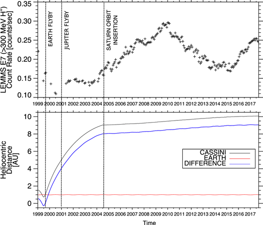
Figure 2. Top: time series of reduced and 26 day averaged >300 MeV GCR count rates from Cassini LEMMS channel E7. Bottom: time series of heliocentric distances of Cassini and Earth, and their difference. In both panels, marked are the times of the Earth and Jupiter flybys and of the Saturn Orbit Insertion (SOI).
Download figure:
Standard image High-resolution imageThe resulting data, along with relevant ephemeris information, are shown in Figure 2.
3.2. GCR Measurements at Earth (1 au): BESS, BESS-Polar, PAMELA, and AMS-02
The measurements by Cassini are compared with GCR observations at Earth (to which we may refer by Earth's heliocentric distance at 1 au). For that purpose, we use data obtained from several advanced GCR observatories (Table 1), namely BESS, BESS-Polar, PAMELA, and AMS-02. All these observatories comprise large magnetic spectrometers capable of retrieving precision differential energy spectra of GCRs with high energy and species resolution throughout the energy range of Cassini's >300 MeV proton measurements. These energy-resolved spectra offer several advantages for our analysis compared to the use of integral flux measurements (e.g., van Allen 1988) or compared to spectral reconstructions based on neutron monitors and theory, as will be presented in Section 3.3.
Table 1. Sources of GCR Proton Measurements at Earth
| Instrument | Energies (MeV) | Dates | Data Sources |
|---|---|---|---|
| BESS | >200 | 1993–2002 | Shikaze et al. (2007) |
| BESS-Polar | >200 | 2004, 2008 | Abe et al. (2016) |
| PAMELA | >80 | 2006–2016 | Adriani et al. (2013), Martucci et al. (2018) |
| AMS-02 | >430 | 2011–today | Aguilar et al. (2013, 2018) |
Note. The date ranges for BESS and BESS-Polar do not indicate the periods between which continuous measurements were obtained, but the time periods containing the several short-duration flights of the respective experiments. All experiments obtain (or have obtained) differential GCR proton flux spectra above the energies indicated in the second column. We note that AMS-02 measurements may reach down to 150 MeV. GCR proton spectra by AMS-02, however, are provided only above ∼430 MeV (Aguilar et al. 2018). The upper energy bound at which fluxes are energy-resolved is well above the energy range where LEMMS has any appreciable GCR sensitivity (∼10 GeV; see Figure 6).
Download table as: ASCIITypeset image
Among the different observatories, BESS and BESS-Polar were high-altitude balloons operated for 12 short-duration missions between 1993 and 2008. Only the five missions after 1999 (1999, 2000, 2002, 2004, 2008), when Cassini's MIMI/LEMMS was functional, are relevant here. PAMELA and AMS-02 operated or still operate on long-duration orbital missions, offering time series of GCR spectra nearly continuously since 2006. Certain measurements by BESS-Polar, PAMELA, and AMS-02 overlap in time such that small differences between the respective spectra can be evaluated and cross-calibrated. The BESS flight in 1999 overlaps both in space and time with Cassini's Earth flyby, as mentioned in Section 2.
GCR spectra from the aforementioned experiments were subject only to minor processing described below:
- 1.All GCR spectra were interpolated at common time and energy tags, such that simultaneous measurements can be compared and cross-calibrated, when available. Linear interpolation was used for GCR time series at a fixed energy, while logarithmic interpolation was applied for GCR fluxes as a function of energy.
- 2.AMS-02 spectra where extrapolated from their minimum energy at 430 MeV (Table 1) down to the lowest energy where LEMMS E7 responds (∼300 MeV) as this is necessary for reconstructing the LEMMS count rate in one of our analysis steps introduced in Section 4.2. Extrapolation was performed through an analytical spectrum function (Section 3.3), requiring that its flux at 430 MeV matches the one measured by AMS-02. This extrapolation has negligible impact on our results because of the relatively narrow energy range involved and the low GCR fluxes between 300 and 430 MeV and is primarily done for the application of several numerical integrations starting from the ∼300 MeV threshold.
- 3.PAMELA fluxes were divided by an energy-dependent scaling factor, P(T) (T: energy). This factor was estimated by time-averaging the energy-dependent ratio of simultaneous PAMELA and AMS-02 spectra after 2011. For the energy range of interest, that ratio ranged between 0.95 and 1.1, indicating good agreement between the two data sets even without correction. For most energies, the PAMELA fluxes were slightly higher than that of AMS-02 (P(T) > 1). The reason we adjusted PAMELA fluxes to match AMS-02 and not the other way around is that PAMELA fluxes were similarly larger than those estimated from the second BESS-Polar flight in 2008. This choice on how to match PAMELA and AMS-02 fluxes has some minimal impact on our final results, which will be discussed in Sections 5.1 and 6.
- 4.Since proton spectra from BESS are provided until 20 GeV (Shikaze et al. 2007), we extended them manually to 100 GeV. To do that, we estimated the spectral index from measurements between 15.0 and 20.0 GeV for each of the BESS spectra, and we used that to extrapolate them as a power law above that energy. This extrapolation has a negligible impact on our results and was only performed such that several numerical integrations described in Section 4 can be performed. This procedure does not concern spectra from BESS-Polar that are available up to 156 GeV (Abe et al. 2016).
Example time series of 0.5 and 2.0 GeV proton fluxes are shown in Figure 3. By adjusting slightly only the fluxes of PAMELA, simultaneous measurements by the three experiments are in excellent agreement, with differences in fluxes rarely exceeding 1%.

Figure 3. Time series differential GCR proton flux measurements by different observatories at 1 au (top: 0.5 GeV, bottom: 2.0 GeV). The measurements by PAMELA have been scaled by a small amount to better match those from BESS and AMS-02 (see text for explanation).
Download figure:
Standard image High-resolution image3.3. Analytical Description of GCR Spectra
While our analysis relies on measured GCR fluxes, an analytical approximation for the GCR proton spectra can provide useful, practical context. This context information is important for assessing aspects of LEMMS's calibration or results from combined Cassini and 1 au measurements before 2006, which are only available for four isolated intervals (Figure 3). They also serve to complete the missing spectral information of AMS-02 below 430 MeV (Section 3.2).
The reconstruction that we employ here is based on the force-field approximation (Gleeson & Axford 1968), which offers a sufficiently good prediction of the GCR spectral shape and fluxes above 300 MeV that it is applicable for the heliospheric distance range of 1–10 au and serves well the purposes for which we intend to use reconstructed spectra in the present study (Usoskin et al. 2017; Roussos et al. 2019). The GCR differential proton flux spectrum, j(t, T), at a given time (t) and kinetic energy (T) is controlled through a single free parameter, the so-called modulation potential (ϕ[GV]). In the case of protons, it can be represented in units of energy as Φ[GeV] = e ϕ, with e the electron charge. The regulation of this parameter by the solar activity is the way in which force-field spectra are modulated. The equation of the GCR spectrum is as follows:
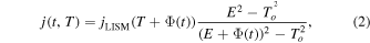
with E = T + To[GeV] being the total proton energy and To = 0.938 GeV the proton rest mass. The spectrum of the local interstellar medium (jLISM) in Equation (2) is given by
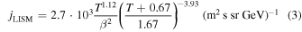
with β = v/c the ratio of the proton speed to the speed of light. Time series of ϕ have been calculated at 1 au by Usoskin et al. (2017) and are regularly updated at http://cosmicrays.oulu.fi/phi/phi.html. The calculation of ϕ is obtained through neutron monitor observations that have been cross-calibrated with PAMELA (Usoskin et al. 2017).
While the force-field approximation achieves a good, first-order representation of the GCR fluxes in the inner heliosphere, it also shows nonnegligible deviations from the measured spectra with amplitudes that depend on the solar-cycle phase. These deviations, which partly stem from the approximation's incomplete physics (Caballero-Lopez & Moraal 2004; Moraal 2013), peak around solar maximum, with fluxes that can be overestimated by as much as a factor of two (Gieseler et al. 2017; Corti 2019). This time-dependent deviation may translate into an artificial solar-cycle dependence of the radial gradient, which is why this analytical reconstruction is mostly used here for context, as explained in the beginning of this subsection.
4. GCR Radial Gradient Estimations
In order to increase the robustness of our analysis, we have developed two different approaches for calculating values of Gr. These are described in the following subsections.
4.1. Method 1: Differential Flux Conversion
In this method, we try to find if LEMMS's channel E7 can be described by a characteristic effective energy (Teff), for which we can convert its count rate to differential flux. In that case, the gradient can be directly estimated through Equation (1), since fluxes at 1 au are energy-resolved. We describe this approach below.
The simplest method for converting channel count rates (R) to differential fluxes (j) is through Equation (4):

where G is the average, omnidirectional geometry factor within the channel's energy interval  . The characteristic energy for j is at the geometric mean of the channel boundaries, that is, at
  (Kronberg & Daly 2013). Since the response of LEMMS's E7 channel is integral in energy, this approximation cannot be used. Instead, because for a differential energy spectrum, j(T), the count rate can be approximated as

then from Equation (4) we obtain the count rate to flux conversion factor, g:

In order to evaluate g, we need to use a predefined spectral form for j(T). This form is given through Equation (2), which is a valid approximation of the GCR spectrum between 1 and 9.5 au. For the E7 geometry factor G(T), we use the profile of Figure 1, integrated over the polar angle (see Figure 9 in the Appendix). Integration limits ( ) are between 100 MeV and 100 GeV. A limitation is that for all of Cassini's positions besides its crossing from 1 au, Φ is unknown. We therefore evaluate the energy profile of g(T) for different, realistic values of Φ. The results are shown in Figure 4 (left). The same calculation can be performed using the spectra measured by BESS, PAMELA, and AMS-02. These spectra are detailed enough that the shape of j(T) can be resolved through measurements only. Here we obtain different spectra by sampling them from different time periods. Evaluation of Equation (6) for this case is shown in Figure 4 (right). We stress that for both cases, estimation of g(T) depends only on the spectral shape, not on the absolute GCR fluxes. Assuming that the spectral shapes within 9.5 au are similar, we may rely on 1 au measurements and approximations to estimate g(T) for any time period of the Cassini mission.

Figure 4. Bow-tie analysis for the response of channel E7 to the spectrum type of Equation (2) and for variable Φ values. The value of g (Equation (6)) is weakly dependent on Φ for T = 2.15 GeV.
Download figure:
Standard image High-resolution imageFor both estimations, we observe that around 2.0–2.2 GeV, all g(T) curves converge toward a single energy and g values that are independent of the chosen Φ (left) or date (right). An effective energy and flux conversion factor for channel E7 (Teff, geff) can be evaluated by finding the centroid of all these curve intersections. Based on the analysis of the measured spectra (Figure 4, right), we obtain that for GCR-type spectra, channel E7 can be described with Teff = 2.0 ± 0.2 GeV and geff = (1.0 ± 0.1)10−4 m2 sr GeV. The method of determining these two parameters is a generalization of the "bow-tie analysis" (Van Allen et al. 1974), typically applied with the use of power-law spectra where the variable input is that of the spectral index.
We can now estimate the differential flux at 2.0 GeV measured by Cassini, requiring also that its value should agree with the 2.0 GeV flux measured by the BESS99 experiment, which occurred close in time to the Cassini flyby. In that case, we obtain
with the factor 4.086 accounting for the aforementioned normalization at 1 au. For this normalization, we compared Cassini data between 0.75 and 1.25 au with those of BESS99. The magnitude of this correction is discussed in the Appendix. We note here that BESS or BESS-Polar measurements require an adjustment that accounts for a small reduction of GCR fluxes at the operational altitude of these spectrometers within Earth's upper atmosphere (Sanuki et al. 2000; Shikaze et al. 2007). This kind of adjustment may introduce some systematic errors in the obtained spectrum. It is thus important that the proton spectrum from BESS99 is in excellent agreement with fluxes from neutron-monitor-based reconstructions or other GCR flux proxies (Gieseler et al. 2017; Usoskin et al. 2017). We therefore do not find a reason to apply any additional correction factor to the BESS99 fluxes, before scaling Cassini's measurements to them.
Applying Equation (7) for Cassini (jCassini) and retrieving from the measurements the 2.0 GeV fluxes at 1 au (jEarth), we obtain the time series shown in the top panel of Figure 5. Following 2001, jCassini is steadily higher than jEarth, as expected for a positive GCR radial intensity gradient. Unfortunately, because GCR spectra at 1 au are not continuously available before 2006, we cannot utilize all of the Cassini observations for our analysis, which are available also for 1999–2006 (Figure 2).
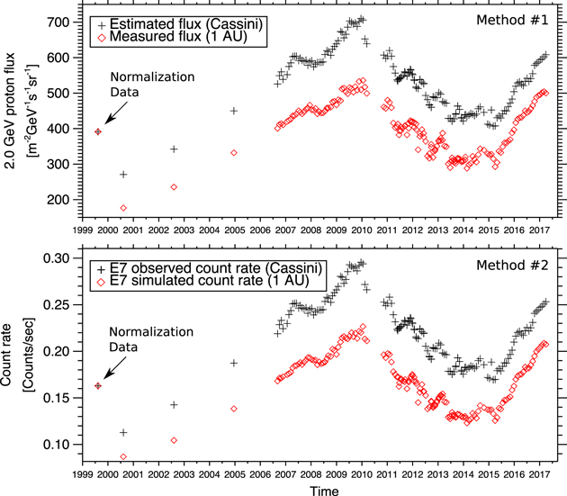
Figure 5. Top: time series of estimated 2.0 GeV proton differential fluxes at Cassini's position (red diamonds) against the measured fluxes at 1 au (black crosses) from BESS, BESS-Polar, PAMELA, and AMS-02. Bottom: time series of the observed LEMMS E7 count rates (black crosses), and the simulated count rates of a virtual E7 channel residing at 1 au (red diamonds). Estimated fluxes and simulated count rates are normalized to the corresponding observations at 1 au, as marked, and are shown only where GCR spectra at 1 au have been obtained directly.
Download figure:
Standard image High-resolution imageA careful inspection of the jCassini time series reveals small differences from the count rate profile of Figure 2, even though the two quantities, based on Equation (7), should be proportional. That is because the profile of jCassini has been time-shifted to account for solar wind propagation effects between 1 au and Cassini and then interpolated back to the time tags of jEarth, such that Equation (1) can be applied. The time shift was performed assuming an average solar wind velocity of 431 km s−1 (Echer 2019; Roussos et al. 2019),
With the data shown in Figure 5 (top), we can apply Equation (1), where j1 = jEarth and j2 = jCassini (Section 4.3). A possible caveat of this method is that the resulting profiles depend significantly on the value of the effective energy, Teff. This is a calibration-sensitive value that affects the time series of jEarth that we choose to compare with, since Teff controls the amplitude of their sinusoidal solar-cycle variation of GCR fluxes that decreases with energy. For this reason, in the following subsection we also apply a method that does not depend on the choice of an effective energy.
4.2. Method 2: LEMMS Count-rate Reconstruction
The second method is driven by the following question: what would have been the count rate of LEMMS's channel E7 had Cassini remained continuously at 1 au? As proton spectra at 1 au are known, we can reconstruct time series of this count rate (REarth) by folding them into Equation (5). At Cassini's position, the count rate (RCassini) is the actual one measured by channel E7 (Figure 2). Similarly, the simulated values of REarth were normalized so that they match the ones measured by Cassini around its Earth flyby. Overall, we obtain

with 4.116 being the normalization factor. Notice that the normalization factor is similar to that of Method 1 (Equation (7)), suggesting that the two methods are complementary. The resulting time series of E7 count rates are plotted in Figure 5 (bottom).
In principle, Equation (1) can be applied even if we set j1 ≡ REarth and j2 ≡ RCassini, assuming that the energy dependence of Gr in the range that E7 receives most of its signal from is secondary. This energy range is rather broad, as we illustrate in Figure 6. The GCR contribution to the E7 signal peaks at ∼0.6 GeV (black curve), but other energies are also important. If we apply Equation (5) but with a variable minimum energy integration limit, we obtain the cumulative count rate (Figure 6, bottom, red). This shows that 50% of the total count rate is contained below T = Teff (Section 4.1), while 90% of the E7 signal comes approximately between 0.5 and 10 GeV. Gieseler & Heber (2016) and de Simone et al. (2011) indicate a slightly decreasing Gr between 0.43 and 1.2 GeV. At higher energies, the models predict that the decrease in Gr is stronger. A decrease in Gr at high GCR energies can be deduced directly from observations, since above ∼10–20 GeV, heliospheric GCR fluxes are similar as in the LISM. Alternatively, we may consider Gr in this case to be an integral gradient, as in many past studies (van Allen 1988; Honig et al. 2019).
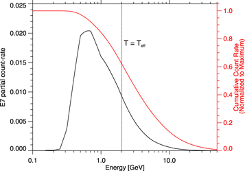
Figure 6. Partial count rate contribution to the GCR signal of LEMMS channel E7 as a function of proton energy (black curve, left vertical axis) for a typical GCR proton spectrum. With red we plot the cumulative count rate normalized to its maximum. The effective energy of channel E7 (Figure 4, Section 4.1) is also marked.
Download figure:
Standard image High-resolution image4.3. Time Series of Radial Gradients
The calculated radial intensity gradient time series using Methods 1 and 2 are shown on the top panel of Figure 7. Time series of averaged Gr values over 4 month intervals and context information from past studies are also shown (de Simone et al. 2011; Gieseler & Heber 2016; Vos & Potgieter 2016; Honig et al. 2019). The monthly sunspot number (http://www.sidc.be/silso/monthlyssnplot), the heliospheric current sheet (HCS) tilt (http://wso.stanford.edu/Tilts.html), and the interplanetary magnetic field magnitude at 1 au from the Advanced Composition Explorer are added for context in the lower panels. We now focus on the the top panel of Figure 7. We may identify two extended time periods, before and after 2006.

Figure 7. Top panel: GCR radial intensity gradient calculated with two methods (black, gray circles). A 4 month average of Gr based on Method 2 data is overplotted with red. Averages based on Method 1 data lead to a very similar profile. Cyan, blue, and orange filled or hatched boxes show estimations from past studies. The gray-hatched box shows the range of Gr values obtained before 2005, where we lack continuous GCR spectra, if the force-field approximation is used to estimate GCR fluxes at 1 au. Bottom panels: time series of the monthly sunspot number, the heliospheric current sheet tilt, and the interplanetary magnetic field magnitude at 1 au. Aspects or events of solar cycles 23 and 24 are also marked in the different panels.
Download figure:
Standard image High-resolution image4.3.1. Radial Gradient: 1999–2006
Data before 2006 are sparse and rely only on three Gr estimates based on simultaneous observations by Cassini and the BESS flights in 2000, 2002, and 2004. The estimate for the year 2000 is between 8%–12%/au from the two methods and is not visible in the scale of the plot. We consider these estimates unreliable for several reasons outlined below:
- 1.The three estimates are isolated and rely only on a few samples by Cassini and BESS that may be affected by transient heliospheric conditions. Indeed, the BESS-2000 flight occurred in the recovery phase of the Bastille Day ICME that disrupted the heliosphere globally (Webber et al. 2002). Similarly, the BESS-2002 flight occurred while Earth was immersed in a Forbush decrease (Shikaze et al. 2007).
- 2.Our two calculation methods for Gr using data from the BESS-2000 and BESS-2002 periods yield different results. Furthermore, a Gr > 8% for 2000 appears extreme.
- 3.Using neutron monitor data to obtain a proxy for GCR spectra at 1 au through the force-field approximation (Section 3.3, Usoskin et al. 2017) results in much lower Gr values compared to those based on BESS between 2000 and 2004 (Figure 7, top, gray-hatched area). While such differences are not unexpected (Section 3.3) and for 2004 they are not unrealistic, no independent derivation of GCR spectra is available that could help us assess which of the two Gr estimates is closer to reality.
We will therefore not consider pre-2006 Gr calculations in the following discussion. These results are nevertheless important for future reference as they illustrate the challenges involved in combining GCR measurements from different data sources, especially when the spectra are resolved for short-duration and isolated time intervals.
4.3.2. Radial Gradient: 2006–2017
The radial gradient after 2006, when PAMELA and AMS-02 spectra are available almost continuously, displays several distinct features. Some of these features may be more easily visible in Figure 8, which zooms into the 2006–2017 period. Shaded areas in Figure 8 are overplotted to guide the eye for identifying short-duration structuring of the Gr profile and several of the following discussion points. We recommend that readers use Figures 7 and 8 in a complementary way.
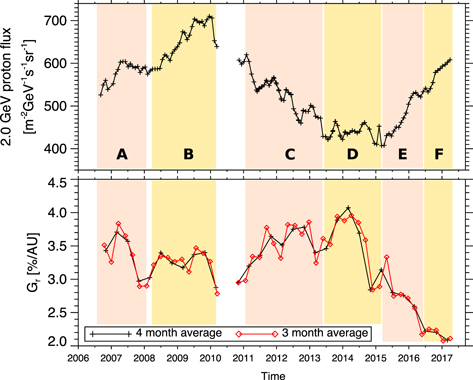
Figure 8. Top: fluxes of 2.0 GeV GCR protons at Cassini, as in Figure 5. Bottom: time series of Gr for a 3 and a 4 month averaging window. In both panels, shaded areas with alternating color highlight several recurring enhancements in Gr or GCR fluxes. The boundaries of these enhancements have been determined "by eye," using either the Gr or the GCR time series. Each of these enhancements is marked with a letter (A–F) to aid the discussion in Section 5.3. The 3 month averaging in Gr indicates that some long-duration events may be more structured (e.g., events B, C).
Download figure:
Standard image High-resolution imageSince both calculation methods give nearly identical results for Gr, we show the long-term average profile from the second method only (Figure 7, top, red line, or Figure 8). Between 2006 and 2014, the gradient is quasi-constant with an average of Gr = 3.5 ± 0.3%/au, with evidence of a broad, weak minimum present between 2008 and 2011. After 2014, Gr experiences a clear, steady drop, reaching 2.0%/au by 2017 September. The dropout begins to develop around the time of the maximum of solar cycle 24 and the full transition to A > 0. Superimposed on this long-term 11 yr profile are hints of faster variations, each lasting between a few hundred days and ∼2 yr. In the following section, we expand on the validation of these results, based on which we proceed with initial physical interpretations of our findings.
5. Discussion
Through the analysis of Cassini LEMMS GCR observations that were obtained between 1999 January and the end of the mission in 2017 September, we have calculated time series of the GCR radial intensity gradient (Gr) between 1 and 9.5 au. For that purpose, we combined LEMMS data with those of advanced energetic particle observatories at 1 au (BESS, BESS-Polar, PAMELA, AMS-02). Certain observations before 2006 were used to achieve an absolute flux calibration of LEMMS's GCR measurements but otherwise offer Gr estimates that cannot be reliably validated. In the following sections, we will therefore elaborate only on the post-2006 results that were presented in Section 3.
5.1. Validation of Gr Time Series
LEMMS was not designed to measure GCRs, which is why we have invested a significant fraction of this study into the absolute GCR flux calibration of LEMMS (see also the Appendix), from the processing of the data and to the validation of our results. Here, we extend the validation efforts by comparing our findings with several independent Gr estimations. Some of these estimates and their uncertainties (de Simone et al. 2011; Gieseler & Heber 2016; Honig et al. 2019) are overplotted as shaded or hatched boxes in the top panel of Figure 7.
Most of these earlier studies provide Gr measurements between 2006 and 2009 July, with Honig et al. (2019) covering several more intervals in 2005, 2009–2011, and 2014. A comparison with the 2006–2011 cluster shows that our Gr values are similar, although they are generally toward the high end of the uncertainty range of those earlier studies. Given the multiple data processing steps and the diversity of the data sets compared, we consider such differences insignificant. A small source of discrepancy, for instance, may be the energy dependence of Gr. The values shown for de Simone et al. (2011) and Gieseler & Heber (2016) are for ∼1.2 GeV, the highest proton energies resolved in these two investigations, while our GCR measurements are more representative for Teff = 2.0 GeV protons (Section 4.1).
In terms of data analysis pipeline, Table 2 summarizes how sensitive our results can be if we treat the cross-calibration between PAMELA and AMS-02 in two different ways (last two rows of Table 2). We find that in both cases, gross features of the Gr variability profile shown in Figures 7 and 8 are retained (e.g., fast drop of Gr after 2014), excluding the transient Gr minimum around the 2009 solar minimum, which cannot be resolved if correction factors to PAMELA and AMS-02 fluxes are obtained by averaging the two data sets at their overlapping time periods (2011–2014). Furthermore, all changes discussed in Table 2 lead to an average drop of the Gr amplitudes by 0.2%–0.5%/au, improving agreement with certain independent estimates, particularly for 2006–2008. We nevertheless consider the differences between the three cases small and the profile plotted in Figures 7 and 8 as representative. Any subsequent discussion points to the profile of those two figures.
Table 2. Impact of Changing the Cross-calibration Approach between PAMELA and AMS-02
| Assumption | Results |
| Adjusting PAMELA to AMS-02 fluxes | See Figures 7, 8 |
| Adjusting AMS-02 to | |
| PAMELA fluxes | Gr profile of Figures 7, 8 shifted uniformly by −0.5%/au. Better agreement with independent Gr estimates for 2006–2008, worse for 2008–2011 |
| Adjusting AMS-02 and PAMELA fluxes to their midpoint values | Quasi-constant Gr profile before 2014 (A < 0); no obvious minimum in Gr for solar minimum in 2009. Better agreement with independent Gr estimates for 2006–2008. Agreement remains good for 2008–2011. The Gr drop after 2014 remains. The Gr profile of Figures 7, 8 is shifted by ∼−0.2%/au |
Note. The top row points to the approach adopted for the present manuscript. The reason this approach was adopted was that a third, independent measurement by BESS-Polar was closer to that of AMS-02 (Section 3.2). The bottom two rows describe the modified approaches.
Download table as: ASCIITypeset image
The biggest discrepancies in Gr are with the study of Honig et al. (2019), who derive much lower gradients for 2005–2006 July and for 2014 January to March. While for the 2005–2006 period we do not have simultaneous estimates, it would seem unlikely that the gradient would change so drastically, from ∼1.6 to 3.4%/au within a few months after 2006 July. We note that the aforementioned calculation of Honig et al. (2019) took place 0.43–0.75 au away from Earth. It is possible that local solar wind dynamics may partly mask global-scale gradients of GCRs over such scales, leading to the small Gr values observed. Other estimates by Honig et al. (2019), farther away from Earth (2008 March–2011 July), are in much better agreement with our derivation.
The same argument cannot explain the even larger discrepancy in 2014. Honig et al. (2019) found that for the period 2014 January to March the gradient between 1 and ∼4.36 au was Gr = 2.13%/au, as opposed to 4.05%/au from our analysis. This measurement by Honig et al. (2019) is based on Rosetta observations from the vicinity of its target comet 67P. After 2014 March, GCR rates measured by Rosetta progressively dropped until they became smaller than those at 1 au, leading to a negative radial gradient and hinting that the comet locally modifies GCR fluxes by some process that is yet to be identified. Even though Honig et al. (2019) considers that before 2014 March the GCR fluxes may be unaffected by the comet, in view of our findings, we advocate that a partial GCR flux reduction could have been present at Rosetta also in that earlier period. What also favors such an interpretation is that Honig et al. (2019) presents GCR proxy data from Mars Odyssey at 1.5 au, indicating a signal comparable to that of Rosetta at 4.36 au before 2014 March. That would imply a considerable radial gradient between 1 au and the orbit of Mars and a vanishing one between Mars and 4.36 au, which would be surprising. We therefore consider that our estimate is more representative of the global radial gradient for 2014. We cannot exclude that additional dependencies, such as a heliocentric distance dependence of Gr, contribute to the differences, but we consider this unlikely, because if that was true, Cassini and Rosetta estimates would have diverged also in earlier time periods (2007–2011).
Based on all these arguments, we are confident that our Gr estimations after 2006 July (Figure 7, top panel) are valid within 0.5%/au. The comparison with independent Gr calculations and possible variations of our data analysis steps indicate that a slight Gr overestimation from our side is more likely than an underestimation. Also, GCR transport models generally predict slightly lower Gr values for few-gigaelectronvolt protons compared to what we find here (Vos & Potgieter 2016). But since our analysis relies on the combination of measurements at a quasi-constant heliocentric distance, with a single data set at 9.5 au and three accurately cross-calibrated data sets at 1 au (Figure 3), we consider that there is little ambiguity regarding the relative temporal Gr variations that we derive compared to past studies. The discussion that follows focuses on the resulting Gr variability pattern.
5.2. Gr Variations at Solar-cycle Timescales
We now turn our attention to the Gr variability trends (Section 4.3). Most of our Gr observations are in solar cycle 24, such that we cannot make extensive comparisons with solar cycle 23. For this study it is more sensible to separate the Gr time series into their A < 0 and A > 0 phases as well as compare solar minimum against solar maximum observations.
A prediction of drift-modulated GCR transport models for the inner heliosphere is that Gr values during the A < 0 phase are larger than those of A > 0 (Burger & Hattingh 1998; Potgieter et al. 1989; Potgieter 2017). This theoretical prediction is in agreement with our observations, where we find that Gr progressively decreases into the A > 0 phase, reaching the lowest estimated values in 2017. This is even more obvious when comparing periods "A" and "F": at similar solar-cycle phases and GCR flux levels (Figure 8), their Gr differs by 1.5%/au, with the highest values for the A < 0 period in 2006–2007. In terms of solar-cycle phase control, our observations also indicate a stronger control for A > 0, when the Gr dropout develops over several years and in line with changes in the various solar indices shown in the lower three panels of Figure 7. For the A < 0 phase, the apparent alignment of the broad Gr minimum with the solar minimum also suggests a solar-cycle control, albeit a much weaker one than for A > 0. Correlation coefficients between Gr and the solar indices are generally positive and highest with the sunspot number and the HCS tilt (values ∼0.5). Due to the long, 4 month averaging used and the limited Gr data set, introducing time lags for exploring higher correlation coefficients does not yield clear results.
Our observation of a peaked and a transient Gr minimum toward solar maximum and solar minimum, respectively, is consistent with several Gr calculations for previous solar cycles (van Allen 1988; Webber & Lockwood 1991). Such a solar-cycle control may have a straightforward explanation: assuming a static GCR LISM spectrum, the difference between LISM fluxes and those within the heliosphere are the greatest during solar maximum, when heliospheric GCR fluxes reach their minimum levels (or the contrary). A difference with those earlier studies, however, is that they report similar Gr values on each side of the solar maximum, indicating a stronger control by solar-cycle phase (e.g., sunspot number), rather than from the polarity of the solar magnetic field. We cannot assess whether these disagreements signify issues in certain observations, differences between (odd/even) solar cycles, or a combination of the above.
5.3. Short-term Gr Variations
As briefly mentioned in Section 4.3.2, the Gr time series display variations also on yearly or biennial timescales, most clearly visible in Figure 8. Several Gr changes before 2015 are apparent as enhancements bounded by clear minima (marked as A–D). After 2015, enhancements E and F are more subtle but still visible. The enhancements have a visible correspondence in GCR fluxes for events A, B, E, and F. Events C and D are more obvious in lower energy GCR measurements by LEMMS and at 1 au (Figure 3, Roussos et al. 2019).
Pizzella (2018) observed that many such features in GCR intensities at 1 au tend to recur every several hundred days. Since a similar recurrence was seen at 9.5 au, Roussos et al. (2019) argued that these are heliospheric modulations corresponding to the so-called quasi-biennial oscillations (QBOs). These are quasi-periodic variations of the solar magnetic field with a broad range of periods in the 0.6–2.0 yr range (Bazilevskaya et al. 2014) that propagate in the heliosphere and may modulate accordingly the GCR spectra (Krivova & Solanki 2002; Obridko & Shelting 2007; Mandal et al. 2017). Uncertainties and the long-averaging of our Gr time series prevent us from exploiting the full QBO periodicity range with accuracy. A Lomb–Scargle periodicity analysis (not shown here) leads to a noisy spectrum with several peaks in the expected range for QBOs. The durations of individual Gr enhancements and their alignment with corresponding features in GCR intensities are what gives some credence to the link between QBOs and the short-term variability of Gr.
There are several ways that QBOs may leave signatures in radial GCR gradients. One possibility is that their appearance is an artifact that is due to the fact that for the alignment of GCR observations at 1.0 and 9.5 au we are using an average solar wind velocity of 431 km s−1 (Echer 2019; Roussos et al. 2019) for the whole time period analyzed. Large deviations from this velocity may lead to a misalignment of QBO events in GCR intensity and thus lead to an artificial gradient roughly at the time of each event's occurrence. We do not believe this to be the case here, since uncertainties in solar wind propagation times between 1 and 9.5 au may be as large as a week but only for rare extreme events. Propagation uncertainties are also small compared to our 26 day averaging of the GCR intensities, the 3–4 month averaging of the Gr series, and the duration of the QBO events.
For instance, the peak of event "A" in GCR fluxes at 9.5 au (Figure 8, top) is misaligned by several months to the corresponding 1 au feature (Figure 5). This misalignment is too large to be attributed to an error in solar wind propagation. The much better aligned event "B" features much sharper changes in GCR fluxes at 9.5 au, explaining the similarly sharp decrease in Gr at its outset in early 2010. These two examples suggest that QBO properties (spatial extent, intensity) evolve from the inner to the outer heliosphere, leading to transient variations of Gr across large spatial scales, in the same way that the merging of interaction regions in the heliosphere may lead to similar effects (Potgieter et al. 1993; Potgieter & Le Roux 1994; Wang & Richardson 2002). It is, however, questionable whether global merged interaction regions had a big impact during the latter two quiet solar cycles (Luo et al. 2019).
6. Summary
The analysis of Cassini measurements in conjunction with highly resolved GCR proton spectra by BESS, BESS-Polar, PAMELA, and AMS-02 enabled us to determine the variability of the proton GCR radial intensity gradient (Gr) for a period that exceeds a full solar cycle (2006 July to 2017 September) and for a quasi-constant heliocentric distance range (1–9.5 au). Our principal result is that after 2006, when Gr is best determined, gradient variations are resolved over both long (solar cycle) and short (yearly) timescales. The magnitude of the gradient ranges mostly between 2% and 4%/au, in agreement with past investigations.
The long-term variability appears to have two components. The first component is associated with the polarity sign of the solar magnetic field. The strongest gradients were observed during the A < 0 phase, until mid-2014, in agreement with predictions by drift-modulated GCR transport models. The transition to lower Gr values in the A > 0 phase develops over several years. The second component concerns the control of Gr by the solar-cycle phase. For A < 0, Gr appears to attain a subtle minimum during the long solar minimum of 2009. For A > 0, correlated variations of Gr with solar indices (sunspot number, HCS inclination) seem stronger. The Gr peaking around the time of the solar maximum has been observed also for previous solar cycles (van Allen 1988; Webber & Lockwood 1991).
Short-term variations consist of recurring Gr enhancements, each lasting several hundred days. Several of these enhancements have clear corresponding signatures in GCR intensities at both 1 and 9.5 au. We attribute these features to QBOs, which are observed in various heliospheric indices. Their presence in GCR radial gradients may offer hints on how QBOs evolve spatially and temporally as they propagate to larger heliocentric distances and the way they impact GCR spectra. Peak-to-valley amplitudes of these short-term enhancements reach up to ∼0.5%/au.
Our calculations were compared and validated against estimations of Gr by independent studies. Because several differences from past investigations do exist, we refrain from generalizing our findings to any solar cycle and consider them representative only for solar cycles 23 and 24 and for proton energies in the low gigaelectronvolt range. We also recognize that the multiple data analysis steps and the diverse data sets that we combined may lead to systematic errors in Gr that are difficult to assess and quantify. It is our view that these errors are more likely to shift the Gr time series up to −0.5%/au as a whole, rather than randomly scatter each individual Gr estimate. We cannot, however, exclude slight changes in the variability pattern, most notably affecting the coincidence of Gr minima/maxima with solar minimum and maximum, respectively (Section 5.1, Table 2).
Given the limitations in estimating some uncertainties, our study will benefit from further validation. We believe that the methodology we introduced here should be readily applicable to many other GCR observations that have been taking place in the heliosphere in the time frame of BESS, BESS-Polar, PAMELA, and AMS-02. The absolute flux calibration of Cassini may allow us to compare its measurements with those of Ulysses, Mars orbiters, and New Horizons and also estimate latitudinal gradients. New Horizons, for instance, crossed Saturn's orbit between 2008 and 2009 and can resolve GCRs in the same way as Cassini (Hill et al. 2018; Kollmann et al. 2019). Such investigations would add another dimension to the observations of the inner heliosphere, which we expect will be crucial for understanding GCR transport and dynamics.
We thank Andreas Lagg and Markus Fränz (MPS) for extensive software support and Martha Kusterer and Jon Vandegriff (both JHUAPL) for reducing the MIMI data. Cassini data analysis at MPS was supported by the German Space Agency (DLR) through contracts 50 OH 1101 and 50 OH 1502 and by the Max Planck Society. E.R. and K.D. also acknowledge the support by NASA grant 18-DRIVE18 2-0029, Our Heliospheric Shield, 80NSSC20K0603, and useful discussions with SHIELD team members (http://sites.bu.edu/shield-drive/). We are grateful to ASI for the data services provided through the Cosmic Ray Database (https://tools.ssdc.asi.it/CosmicRays/).
Appendix: Notes on the LEMMS GCR Calibration
As the present investigation required us to analyze Cassini LEMMS data from 1999, we have processed the instrument's housekeeping data and reviewed relevant documentation in order to reconstruct any changes in the instrument's calibration before the Saturn tour. The LEMMS channel responses are determined by the coincident energy losses of particles that hit different solid state detectors (SSDs). SSDs are triggered only if the energy loss exceeds a given threshold. LEMMS had programmable thresholds, which changed five times throughout the mission for testing or optimization of the instrument. These time periods are listed below:
- Calibration period 0: 1999-003T00:00:00 to 2000-193T23:08:23
- Calibration period 1: 2000-193T23:08:23 to 2000-207T21:10:54
- Calibration period 2: 2000-207T21:10:54 to 2000-293T06:50:00
- Calibration period 3: 2000-293T06:50:00 to 2003-264T00:07:00
- Calibration period 4: 2003-264T00:07:00 to 2004-295T04:01:21
- Calibration period 5: 2004-295T04:01:21 to 2017-259T00:00:00
Specifically for channel E7, threshold settings and its response function were similar for periods 0, 3, 4, and 5 (Figure 9). The broader and strongest response was in Calibration period 1, where E7 can capture protons of slightly lower energy (>250 MeV) compared to other periods (>300 MeV). The weakest response is in Calibration period 2, where the geometry factor for gigaelectronvolt protons drops by a factor of ∼2.
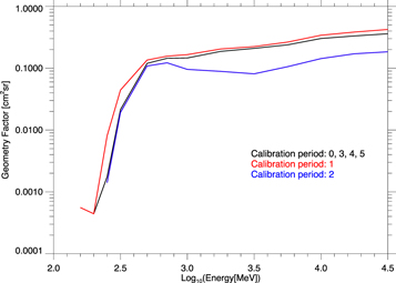
Figure 9. Omnidirectional proton response function of LEMMS channel E7 for different calibration periods.
Download figure:
Standard image High-resolution imageData around the period of Calibration periods 1 and 2 are shown in Figure 10. Unlike Figure 2, data here are daily averaged, while data around ICME events, the Jupiter flyby, and the two aforementioned calibration periods were not filtered, in order to illustrate aspects of the processing discussed in Section 3.1.
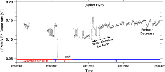
The data in Figure 10 show that at the transition from Calibration period 0–1 (strongest response), count rates experience a clear increase, while during the transition to Calibration period 2 (weakest response), a sharp drop is observed. If we normalize the measurements to Calibration period 0, then the ratio of count rates for periods 1–3 is 1:1.22:0.48. At that time period, the GCR modulation potential was between 0.7 and 0.9 GV and the heliocentric distance of Cassini was ∼4.5 au, where the modulation potential should be ∼5% weaker (Caballero-Lopez & Moraal 2004). Using these parameters, we estimate, using Equations (2) and (5) and the response functions shown in Figure 9, that the count rate ratios should be 1:1.11:0.54 (0.7 GV) and 1:1.11:0.52 (0.9 GV), close to the observed values. Differences can be attributed to deviations of the simulated response function from the actual one or the use of the force-field approximation to reconstruct count rates for that time period.
Figure 10 shows also daily average data from the Jupiter flyby and the period after it, which were filtered for our main analysis. The closest approach to Jupiter is clearly identified as a sharp increase in the E7 count rates. For about 60 days after that spike, GCR levels appear slightly elevated. In both cases, these come from the >7 MeV electrons that E7 was originally designed to measure in Saturn's radiation belts, explaining why such a long period after the Jupiter flyby had to be removed. Relevant observations, but for lower energy electrons, are discussed in Krupp et al. (2002). An example of a Forbush decrease at the end of the plotted interval is also marked. Similar events also had to be removed.
Figure 10. LEMMS E7 channel count rates for the time period of the Jupiter flyby, which included three changes in the LEMMS calibration settings. Several features in that time period (Jupiter flyby, Jovian electrons, Forbush decrease) are marked. The rates are daily averaged and less filtered than those shown in Figure 2.
Download figure:
Standard image High-resolution image
Finally, we briefly comment here on the reconstructed E7 GCR count rate value from Equation (5) compared to the measured one, lower by a factor of ∼4.1. This difference cannot be attributed to the fact that in our model GCR spectra we do not include other species, such as electrons or heavy ions. Even the sum of all those species' contributions would increase the reconstructed count rate marginally, since GCR electron fluxes are very low while LEMMS is much better shielded from heavy ions. The lower simulated rates for the E7 channel may reflect a lower detection efficiency that is due to noise in the detector amplifier electronics or differences in the actual versus simulated detector shielding. We recall that the instrument model used in response function simulations was based on old mechanical drawings (Roussos et al. 2018b), so uncertainties in several of its shielding elements naturally exist. A slightly weaker overall shielding would have resulted in a stronger response function for lower GCR energies, sufficient to account for a large part of the factor of ∼4.0 count rate discrepancy.
We finally note that in Roussos et al. (2019), estimated count rates were larger than those observed because of a error in multiplying Equation (5) with a factor of 4π, although this factor was effectively included in the omnidirectional geometry factor. Results of that study are not affected by that error, as only the relative variations and periodicities of the GCR rates were relevant for the conclusions and not the absolute LEMMS flux calibration. The only change would be that the constants k in Table 1 of that manuscript should be divided by 4π.