


Abstract
We report on the results of a new spectroscopic monitoring campaign of the quasar PG 0026+129 at the Calar Alto Observatory 2.2 m telescope from 2017 July to 2020 February. Significant variations in the fluxes of the continuum and broad emission lines, including Hβ and He ii, were observed in the first and third years, and clear time lags between them are measured. The broad Hβ line profile consists of two Gaussian components: an intermediate-width H with an FWHM of 1964 ± 18
  and another very broad H
 with an FWHM of 7570 ± 83
  . H
. H has long time lags of ∼40–60 days in the rest frame, while H
 shows nearly zero time delay with respect to the optical continuum at 5100 Å. The velocity-resolved delays show consistent results: lags of ∼30–50 days at the core of the broad Hβ line and roughly zero lags at the wings. H
 has a redshift of ∼400
  , which seems to be stable for nearly 30 yr by comparing with archived spectra, and may originate from an infall. The rms spectrum of H
 shows a double-peaked profile with brighter blue peak and extended red wing in the first year, which matches the signature of a thin disk. Both the double-peaked profile and the near-zero lag suggest that H
 comes from a region associated with the part of the accretion disk that emits the optical continuum. Adopting the FWHM (in the rms spectrum) and the time lag measured for the total Hβ line, and a virial factor of 1.5, we obtain a virial mass of
  for the central black hole in this quasar.
Export citation and abstract BibTeX RIS
1. Introduction
The broad emission lines are one of the most prominent features of active galactic nuclei (AGNs; see Gaskell 2009 for a review). They are widely used for classification (type I/II and the unification model, e.g., Antonucci 1993; and narrow-line Seyfert 1 galaxies, NLS1s, e.g., Osterbrock & Pogge 1985), measuring the mass of the central black hole (by both reverberation mapping and a single-epoch spectrum; see Peterson 2014 for a review), and studying the physics (by the so-called Eigenvector 1; Boroson & Green 1992) and evolution (e.g., Wang et al. 2012) of AGNs. Hβ is the most studied broad line in the optical spectra of AGNs. However, the geometry and kinematics of its emitting region are still far from well understood. Various complex physical processes and dynamics other than simple virial motions have been suggested to characterize this region, e.g., wind (Murray et al. 1995), inflow (Zhou et al. 2019) and outflow (Czerny & Hryniewicz 2011), and tidal disruption of clumps from the dusty torus (Wang et al. 2017). The observational evidence is often difficult to thoroughly interpret for two reasons: the profiles of Hβ broad lines in different objects are highly diverse, and the variability behavior of the line in a single object is also complex and changeable on a timescale of a few years.
The profiles of the broad Hβ emission lines are often shifted relative to the narrow lines and more or less asymmetric (e.g., Boroson & Green 1992), and generally cannot be described well by a single simple analytical function (e.g., a Gaussian or Lorentzian; see Hu et al. 2012 for a review), indicating that multiple physically distinct components may exist in the Hβ-emitting region. The two-component model for AGNs, including an intermediate-width component and a very broad component, 13 has been proposed in the literature by many authors, as a spectral decomposition of the Hβ profile to two Gaussians or a Gaussian plus a Lorentzian (e.g., Corbin 1995; Brotherton 1996; Popović et al. 2004; Hu et al. 2008a; Marziani et al. 2009; Kovačević et al. 2010). However, the emission-line profile emitted from a single physical component is not necessarily a simple Gaussian or Lorentzian. For example, a thin disk is believed to emit an asymmetric double-peaked profile, which has been observed in many objects (Eracleous & Halpern 1994; Strateva et al. 2003; Storchi-Bergmann et al. 2017). So spectral principal component analysis, as a model-independent approach, has been performed to samples of quasar spectra, and the scenario of two kinematically distinct Hβ components is still favored (Hu et al. 2012).
On the other hand, a scenario of multiple broad-line regions (BLRs) has been suggested from a theoretical perspective by many authors. Netzer & Marziani (2010) found that at least two populations of clouds are required in their calculations to reproduce the observed line profiles, and simple models with only one zone can be ruled out. Wang et al. (2014) calculated the self-shadowing of the super-Eddington accreting slim disk, suggesting the possible existence of two BLRs. Numerical simulations of photoionized gas by Adhikari et al. (2016) showed the production of intermediate-width emission lines in high-density gas because of the inefficient dust suppression.
More interestingly, multiple Hβ broad-line components are also expected for supermassive binary black hole systems, in which the two components relate to different central black holes and have different velocity shifts (e.g., Boroson & Lauer 2009). Alternatively, for rapidly recoiling black holes (e.g., Eracleous et al. 2012), one black hole is "kicked" out during the merger and has a large offset velocity relative to the host galaxy. Thus, besides searching the evidence of multiple emission-line components by statistics in large samples, it is more valuable and convincing to identify such a phenomenon in individual objects. And furthermore, it is important to distinguish whether the multiple components are emitted from physically distinct regions of a single black hole, or related to different black holes.
The identification of multiple emission-line components in individual AGNs is often achieved by performing multi-epoch spectroscopic observations and recognizing the independent variations of different components. Sulentic et al. (2000) observed, in quasar PG 1416−129, that the narrower "classical" broad Hβ component declined dramatically while the very broad component persisted in two spectra taken 10 yr apart. For binary black hole systems, not only the strengths but also the velocity shifts of the emission-line components are expected to have periodical variabilities. By decomposing the broad emission line to several components and studying the variations in their velocity shifts from long-term spectroscopic monitoring, several supermassive black hole binary systems have been claimed in the literature, e.g., NGC 4151 by Bon et al. (2012), and NGC 5548 by Li et al. (2016) and Bon et al. (2016).
The existence of multiple BLRs is more convincing if they are not only kinematically distinct as suggested above, but also geometrically separated. An explicit result of the virialization of two populations of clouds with different velocities is that they will rotate at different distances to the central supermassive black hole. Thus, the reverberation mapping (Blandford & McKee 1982) method would be able to identify multiple broad-line components by detecting different time lags between the variations of separated components and that of the ionization continuum. The time lag represents the distance, because it is the time the ionization photons take to travel from the central continuum source to the ionized line-emitting gas. Bian et al. (2010) and Zhang (2013) attempted to decompose the Hβ broad line into two components, and then measure the time lag of each by reanalyzing the spectroscopic monitoring data of Kaspi et al. (2000) for PG 1700+518 and PG 0052+251, respectively. But the quality of the data sets (mainly the low sampling cadence) allowed no significant detection of two well separated time lags.
Similar to the complexity of the line profile discussed above, a single emission-line component does not need to have a single time lag. It more probably shows complex structure on the velocity-delay map, which could be recovered from high-quality data (by, e.g., the maximum-entropy method; Horne 1994). The results will be much more complicated in the case of two kinematically distinct BLRs with comparable size as simulated in Wang et al. (2018), although the current data quality is not good enough to reveal such fine structures. The velocity-delay maps, or at least high-quality velocity-resolved delays, have been measured for many objects in several campaigns (e.g., Bentz et al. 2009; Denney et al. 2009; Grier et al. 2013b; Du et al. 2016, 2018a; De Rosa et al. 2018; Xiao et al. 2018), showing diverse kinematic signatures including outflowing, infalling, and virialized motion. It turns out that the kinematics drawn from the velocity-delay map does not always agree with that given by profile decomposition. The high-quality velocity-delay map of NGC 5548 recovered by Xiao et al. (2018) suggests a Keplerian disk, rather than two separated BLRs in the scenario of a supermassive black hole binary preferred by the profile analysis mentioned above. Even an intermediate-width long-lag component and a very broad short-lag component do not have to be emitted from two geometrically separated BLRs. For example, in a model of circular Keplerian orbits shown in Figure 10(a) of Bentz et al. (2009), if the line profile is decomposed to two components, one representing the line core and another covering the wings, then the core component will have a longer lag than the wing component. Thus, conclusions drawn from only profile analysis should be reexamined with caution, by taking at least velocity-resolved delays into consideration.
Recently, the direct modeling method (Pancoast et al. 2011) has been developed and applied to roughly a dozen AGNs (e.g., Pancoast et al. 2014; Grier et al. 2017; Li et al. 2018) to measure the black hole masses. By establishing a theoretical model of the motions of the BLR clouds and fitting the yielded line profile variations to the observed reverberation mapping data, the geometry and kinematics of the BLR can be constrained. Li et al. (2018) found that a two-zone model is favored for Mrk 142, although a complicated one-zone model still cannot be ruled out. With improvements in both the observed data and theoretical modeling (see Mangham et al. 2019 for a discussion), this method would hopefully be able to confirm the existence of two distinct dynamical components, and distinguish whether they come from two BLRs of a single black hole or just different black holes in a binary.
This paper presents strong observational evidence for the existence of two separated Hβ-emitting regions in the quasar PG 0026+129. Both the profile decomposition and velocity-resolved delays suggest that the very broad component is emitted from a disk adjacent to the optical continuum source, while the intermediate-width component probably originates from an infall far away. Section 2 briefly describes the observations and data reduction of our recent spectroscopic monitoring of this object using the Centro Astronómico Hispano-Alemán (CAHA) 2.2 m telescope. Section 3 presents the spectral decomposition and the measurements of light curves. The analyses of the light curves and the velocity-resolved delays are then given in Section 4. The properties and possible origins of the two broad Hβ components, along with an estimation of the black hole mass, are discussed in Section 5. Section 6 gives a brief summary.
2. Observations and Data Reduction
PG 0026+129 is a bright radio-quiet quasar with a V-band magnitude of 15.4 and redshift z = 0.1454.
14
The FWHM of its broad Hβ line, given by Boroson & Green (1992), is 1860  , allowing it to be classified as an NLS1. With regards to the other typical spectral features of NLS1, the Fe ii emission is just moderately strong while [O iii] lines are far from weak in this object (see Figure 2 below for an impression). The Hβ profile clearly has strong broad wings.
PG 0026+129 has been monitored once by Kaspi et al. (2000), and a time lag of  days was obtained for its Hβ. Only 56 spectroscopic epochs were observed in ∼7.5 yr. Data with such a low cadence should be dealt with using caution, as the time lag measured could be overestimated by undersampling, as in the case of PG 2130+099 (see discussions in Grier et al. 2008 and Hu et al. 2020). Moreover, obtaining results beyond an averaged time lag, e.g., velocity-resolved delays, requires higher sampling cadence.
Since 2017 May, we started a large reverberation mapping campaign using the CAHA 2.2 m telescope at the Calar Alto Observatory in Spain, which is still ongoing. This campaign is an expansion of the super-Eddington accreting massive black hole (SEAMBH) project (Du et al. 2014), performing long-term and high-cadence spectroscopic monitoring of PG quasars (PG refers to the Palomar-Green Survey; Schmidt & Green 1983) with high accretion rates. The first result of this campaign has been presented in Hu et al. (2020), on an unexpected change of the BLR structure in PG 2130+099 during only two years. The details of the observations and data reduction of this campaign have been described in Hu et al. (2020), so we only briefly present those relevant to PG 0026+129 below.
PG 0026+129 was observed for 47 epochs between 2017 July and 2018 February (hereafter the observations in 2017), 41 epochs between 2018 June and 2019 February (hereafter the observations in 2018), and 39 epochs between 2019 August and 2020 February (hereafter the observations in 2019). For each epoch, broadband images and long-slit spectra were taken by the Calar Alto Faint Object Spectrograph (CAFOS). On the spectrophotometric flux calibration, we follow the strategy in Kaspi et al. (2000) and Du et al. (2014), which requires rotating the slit to observe a nearby comparison star with the object simultaneously. In this case, the comparison star is a G-type (determined from our spectra) star, located 95'' away from PG 0026+129 with a position angle of 42°.
2.1. Photometry
Utilizing CAFOS's ability to swiftly switch observing modes between direct imaging and spectroscopy, broadband images were also taken for two purposes: (1) confirming that the comparison star is non-varying; and (2) comparing the light curves of the object from photometry and spectroscopy to test the spectrophotometric flux calibration. For each epoch, three exposures of 60 s each were taken with a Johnson V filter. Data reduction followed the standard IRAF 15 procedures, and differential instrumental magnitudes of both the object and the comparison star were obtained relative to the other stars within the field.
Figure 1 shows the V-band light curves for PG 0026+129 (top) and its comparison star (bottom), respectively. The comparison star is rather stable as the scatter in its magnitudes is only ≲0.01 mag. The variability of PG 0026+129 shows significant structure in 2017 and 2019, with amplitudes of nearly 0.2 and 0.1 mag between the maximum and minimum, respectively. But in 2018, PG 0026+129 is almost non-varying in the first ∼170 days, and the standard deviation of its magnitudes for the whole year is only ∼0.02 mag.
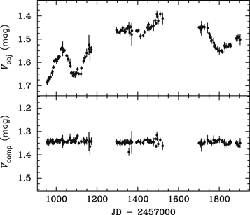
Figure 1. Photometric V-band light curves for PG 0026+129 (top) and the comparison star (bottom), in units of instrumental magnitudes.
Download figure:
Standard image High-resolution image2.2. Spectroscopy
For each epoch, two successive exposures of 1200 s were taken using CAFOS with Grism G-200 and a long slit with a projected width of 30. The spectroscopic images were reduced following the standard procedures using IRAF (see Hu et al. 2020 for details), and then the spectra of both PG 0026+129 and the comparison star were extracted in a uniform aperture of 106. The yielded spectra cover the wavelength range of 4000–8500 Å with a dispersion of 4.47 Å pixel−1. Because the slit is broader than the seeing most of the time, the actual spectral resolution is better than that given by the line width of the wavelength-calibration lamp spectra, and varies in different exposures depending on the seeing. By comparing the widths of [O iii] λ5007 emission lines in our mean spectra with those given by previous high-spectral-resolution observations for several objects in our campaign, we estimated an FWHM of 1000  as the average instrument broadening (Hu et al. 2020). The signal-to-noise ratio (S/N) of PG 0026+129 typically reaches ∼80 per pixel at the continuum around the rest frame 5100 Å for a single exposure.
The flux calibration was done by using the comparison star as a spectrophotometric standard. The details of generating the fiducial spectrum of the comparison star, fitting the sensitivity function, and performing the calibration to the object spectra were described in Hu et al. (2020). The accuracy of the flux calibration by this technique has been proven to be better than ∼3% (e.g., Kaspi et al. 2000; Hu et al. 2020), and the issue of apparent flux variations of the host galaxy (Hu et al. 2015) can be ignored in the case of PG 0026+129 due to its weak host contribution.
The spectra of six epochs are removed from the following light-curve measurements, because of S/N lower than 20 (per pixel around the rest frame 5100 Å), difference between the fluxes of the two exposures larger than 3%, or abnormal spectral slope, all of which were due to bad weather conditions. Thus, the spectroscopic light curves below contain 46 epochs in 2017, 39 epochs in 2018, and 36 epochs in 2019, respectively.
3. Light-curve Measurements
Two methods are often used in reverberation mapping studies for light-curve measurements: integration and spectral fitting. Integration is traditional, and widely used in most campaigns (e.g., Kaspi et al. 2000; Peterson et al. 2004; Bentz et al. 2009; Fausnaugh et al. 2017; Du et al. 2018a, 2018b) for its simplicity and robustness under normal situations. By subtracting the continuum as a straight line defined by two windows, the emission-line flux is measured by a simple integration in a window. This method is suitable for strong, single emission lines such as Hα and Hβ, as long as the continuum can be approximated by a straight line define by the two windows. The spectral fitting technique is relatively new and adopted in fewer reverberation mapping campaigns (e.g., Barth et al. 2013, 2015; Hu et al. 2015). The fluxes of emission lines are obtained from fitting the spectra in a wide wavelength range by including as many spectral components as necessary. This method is useful especially in two situations: (1) for highly blended lines, e.g., Fe ii and He ii, spectral fitting is necessary to decompose them from contaminations (Bian et al. 2010; Barth et al. 2013; Hu et al. 2015); (2) for objects with strong host contribution, the continuum deviates considerably from a simple straight line (Hu et al. 2015, 2016). However, spectral fitting is less robust than integration if the quality of the spectra is not high enough for reliably determining each spectral component, especially the host starlight. In Hu et al. (2020), both methods were used: integration for Hβ and He i, and spectral fitting for Fe ii and He ii.
In this section, we first investigate the uncertainty in measuring the Hβ light curve by the integration method for PG 0026+129, caused by the contamination to the continuum by the broad He ii line. Then, we describe the spectral fitting method, which is preferred in this case due to its better continuum subtraction. Moreover, we obtain the light curves of the two Hβ components decomposed by spectral fitting, both of which seem to have physical meaning.
3.1. Integration
For integrating the flux of Hβ, two continuum windows are used to define a local continuum. The best choice for the redward continuum window is at 5100 Å in the rest frame, in which only very weak Fe ii emission is likely above the continuum (window A in Figure 2, 5085–5115 Å). The blueward window is usually set just adjacent to the blue wing of Hβ, at the local minimum between Hβ and He ii (window B, 4750–4780 Å). However, in this case, the continuum defined by windows A and B is apparently too steep (the green solid line), because of the contamination of broad He ii emission in window B (see the cyan Gaussian in Figure 4). A better choice could be the local minimum blueward of the Hγ line (window C, 4195–4225 Å). The continuum defined by this window, which is much farther away from Hβ, looks more reasonable (the blue solid line in Figure 2).
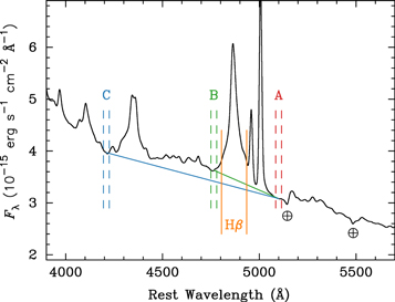
Figure 2. Integration windows for continuum (A, B, and C, between the corresponding pairs of dashed vertical lines) and Hβ line (between the solid orange vertical lines). The green and blue solid lines show the continua defined by windows A and B and A and C, respectively. The spectrum is the mean spectrum, and two telluric absorptions are marked by ⊕.
Download figure:
Standard image High-resolution imageThe top panel of Figure 3 shows the light curve of the continuum at rest frame 5100 Å integrated in window A. It agrees well with that given by the V-band photometry shown in the top panel of Figure 1. The other two panels of Figure 3 show the Hβ light curves measured using different choices of the blueward continuum window: by window B in the middle, and C in the bottom. The fluxes of Hβ are smaller in the middle panel, because more continuum fluxes are subtracted as the result of the contamination of He ii in window B. Moreover, the variability of He ii, which is strong as shown in Figure 6, makes the underestimations of Hβ fluxes vary in different epochs, introducing artificial structures in the light curve. This effect is more severe in 2018, when the variability amplitudes of both continuum and Hβ are small, creating the false illusion of an increasing Hβ flux shown in the middle panel.
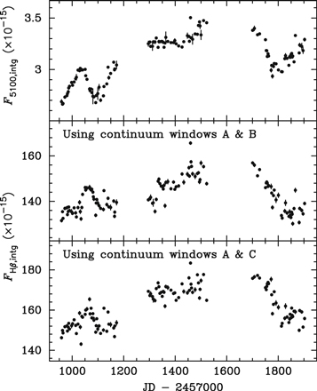
Figure 3. Light curves obtained by integration. Top: continuum at rest frame 5100 Å. Middle and bottom: Hβ above the continua defined by different choices of blueward windows. Note the apparent difference between the two Hβ light curves, indicating the uncertainty in integration method.
Download figure:
Standard image High-resolution imageAlthough window C avoids the contamination of He ii emission, its large wavelength separation from Hβ increases the systematic error introduced by the uncertainty in the spectral shape calibration. Thus, the method of spectral fitting is favored for light-curve measurements in this work.
3.2. Spectral Fitting
Our spectral fitting follows that in Hu et al. (2020), except that the host starlight is not included here. In our spectra, there is no recognizable stellar absorption feature in even the mean spectrum (see Figure 2; note that the two broad absorption features around ∼5145 and 5485 Å are telluric absorptions). Also, the continuum shape in the optical band can be fitted well without adding a starlight component. Thus, we neglect the host in our spectral fitting.
Before fitting, the Galactic extinction correction was performed with an extinction law assuming RV = 3.1 (Cardelli et al. 1989 and O'Donnell 1994) and a V-band extinction of 0.195 mag from the NED determined by Schlafly & Finkbeiner (2011). Then the spectra were de-redshifted with a value of 0.1454, determined by the [O iii] λ5007 line in our mean spectrum.
The following spectral components are included in the fitting, as shown in Figure 4 for a single-epoch spectrum: (1) the AGN continuum modeled as a simple power law, (2) the Fe ii pseudo-continuum generated by convolving a Gaussian with the Boroson & Green (1992) template, (3) the broad Hβ line as two Gaussians, one for the intermediate-width component (H ) and another for the very broad component (H
 ), (4) the broad He ii as a single Gaussian, and (5) narrow emission lines including [O iii] λλ4959, 5007, He ii
λ4686, and Hβ, modeled by a set of Gaussians with the same velocity width and shift. Because of the blending between the Fe ii emission, broad He ii line, and the Hβ wings, and also the degeneracy between the two broad Hβ components, we first fit the mean spectrum with all of the parameters free to vary, and then fit the single-epoch spectra by fixing the velocity widths and shifts of the broad He ii, H
), (4) the broad He ii as a single Gaussian, and (5) narrow emission lines including [O iii] λλ4959, 5007, He ii
λ4686, and Hβ, modeled by a set of Gaussians with the same velocity width and shift. Because of the blending between the Fe ii emission, broad He ii line, and the Hβ wings, and also the degeneracy between the two broad Hβ components, we first fit the mean spectrum with all of the parameters free to vary, and then fit the single-epoch spectra by fixing the velocity widths and shifts of the broad He ii, H , and H
 to the values given by the best fit to the mean spectrum. Also, the relative density ratios between the narrow emission lines are fixed to the values in the best-fit model of the mean spectrum. Among the 20 parameters in total, only 11 are free to vary in the fitting to single-epoch spectra. The fitting is performed between the rest-frame wavelengths 4180 and 5640 Å, excluding a window around Hγ and two narrow windows around ∼5145 and 5485 Å for telluric absorptions.
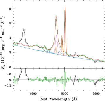
Figure 4. Sample fit of a single-epoch spectrum. In the top panel, the observed spectrum is plotted in green and black for the pixels included and excluded in the fitting, respectively. The best-fit model (red) is the sum of the following components: the power-law continuum and the Fe ii pseudo-continuum (blue), intermediate-width and very broad Hβ components (magenta), broad He ii line (cyan), and the narrow emission lines (orange, including [O iii], Hβ, and He ii). The bottom panel shows the residuals. Two narrow bands around ∼5145 and 5485 Å are excluded in the fitting for telluric absorptions.
Download figure:
Standard image High-resolution imageThe best fit to the mean spectrum yields a nonzero flux of a narrow Hβ component, whose velocity width and shift are forced to be the same as those of [O iii]. The intensity ratio relative to [O iii] λ5007 is 0.156, which is a normal value in AGNs (e.g., Veilleux & Osterbrock 1987). Because of the low spectral resolution in this campaign (instrument broadening ∼1000  ; Hu et al. 2020), the narrow Hβ component is smeared with the redshifted H
 , making the peak of the entire Hβ profile ∼150
  redshifted with respect to [O iii]. It is well known that [O iii], as a high-ionization line, can be blueshifted with respect to the low-ionization lines (e.g., Boroson 2005; Hu et al. 2008b). We checked the spectra of this object obtained with the Sutherland 1.9 m telescope at the South African Astronomical Observatory during this campaign, which have higher spectral resolution (see Appendix B for details). By comparing the velocity shifts of [O iii], [O ii], and the peak of the Hβ profile, we concluded that the [O iii] lines of PG 0026+129 are not blueshifted with respect to the low-ionization lines. Thus, forcing the narrow Hβ component to have the same profile as [O iii] in our fitting is appropriate, and so does using [O iii] to define the systematic redshift when no host absorption feature is available.
Columns (3) and (4) of Table 1 list the FWHMs and velocity shifts of the broad emission lines and components from the best fit to the mean spectrum.
16
The errors are estimated as the standard deviations of the values given by the best fits to Monte Carlo realizations (by bootstrap sample selection) of the mean spectrum. The listed values of FWHMs have been corrected for the instrumental broadening, and those of velocity shifts are with respect to [O iii] λ5007. Note that H is ∼3.9 times broader than H
 . This width ratio is much higher than the average value of 2.5 in Hu et al. (2008a). The width of H
 approximates that of the broad He ii, while H
 and Fe ii (FWHM = 1957 ± 35
  , shift = 243 ± 8
  ) have similar widths.
Table 1. Measurements for Broad Emission Lines and Components
| Line | Flux | FWHM | Shift |

|

| Lag |
|---|---|---|---|---|---|---|
(×10−15
 ) ) | ( ) ) | ( ) ) | (%) | (days) | ||
| (1) | (2) | (3) | (4) | (5) | (6) | (7) |
| 2017 | ||||||
| He ii | 36.0 ± 8.5 | 8445 ± 162 | 1173 ± 62 | 21.3 ± 2.7 | 0.46 |

|
H
| 124.8 ± 7.0 | 7570 ± 83 | 415 ± 12 | 4.4 ± 0.7 | 0.66 |

|
H
| 45.8 ± 3.2 | 1964 ± 18 | 449 ± 3 | 6.7 ± 0.7 | 0.81 |

|
H
| 170.6 ± 6.1 | 3193 ± 141 a | 424 ± 1 | 2.5 ± 0.5 | 0.61 |

|
| 2019 | ||||||
| He ii | 40.1 ± 5.2 | 8445 ± 162 | 1173 ± 62 | 11.8 ± 1.6 | 0.62 |

|
H
| 129.4 ± 5.5 | 7570 ± 83 | 415 ± 12 | 3.9 ± 0.5 | 0.74 | −1.1
|
H
| 51.8 ± 6.0 | 1964 ± 18 | 449 ± 3 | 11.2 ± 1.4 | 0.87 |
 b
b
|
H
| 181.2 ± 8.7 | 3094 ± 133 a | 424 ± 1 | 4.6 ± 0.6 | 0.87 |

|
Notes. Measurements for the broad He ii line, two broad Hβ components, and the total broad Hβ line in years 2017 and 2019. Column (2) lists the mean fluxes, and the errors are the standard deviations. Columns (3) and (4) list the FWHMs after instrumental broadening correction and the velocity shifts with respect to [O iii] λ5007, measured from the mean spectrum, except those for H , which are the means of the values measured from the individual-night spectra. Columns (5) and (6) give the variability amplitudes
  , and the peak values
  of the CCFs. Column (7) lists the time lags τ in the rest frame.
 in 2019 could be underestimated here. See the text for a discussion.
Download table as: ASCIITypeset image
The FWHMs and velocity shifts listed in Table 1 for He ii and two broad Hβ components are identical for different years because we set them to the values measured in the mean spectrum for the entire data set. We tried measuring the mean spectrum of each single year and setting annual averages separately, but the time lags measured in each year have no statistically significant change. However, the relative fluxes of these components between years change, showing some long-term trends. Such trends are not seen in the results here, which could therefore be caused by the varying degeneracy in spectral decomposition if different values are used for different years.
The light curves are generated directly from the fluxes of the decomposed spectral components given by the best fits to the single-epoch spectra. Figure 5 shows, from top to bottom, the light curves of the AGN continuum, the broad He ii, H , H
, H , the total broad Hβ (H
 ), and the Fe ii emission. The flux of H
 is just the sum of the fluxes of H
 and H
and H . Table 2 presents the data of all of these light curves (only the first five epochs are included here as an example; the machine-readable table in its entirety is available online).

Figure 5. Light curves obtained by spectral fitting. From top to bottom: the AGN continuum at rest frame 5100 Å, the broad He ii, the very broad Hβ component, the intermediate-width Hβ component, the total broad Hβ, and the Fe ii emission.
Download figure:
Standard image High-resolution imageTable 2. Light Curves of the 5100 Å Continuum and Emission Lines
| JD−2457000 | F5100 |

|

|

|

|

|
|---|---|---|---|---|---|---|
| (1) | (2) | (3) | (4) | (5) | (6) | (7) |
| 958.663 | 2.559 ± 0.004 | 32.92 ± 0.97 | 119.1 ± 1.2 | 42.27 ± 0.67 | 161.4 ± 0.9 | 66.05 ± 1.39 |
| 962.626 | 2.560 ± 0.003 | 33.16 ± 0.76 | 120.1 ± 1.0 | 44.72 ± 0.55 | 164.9 ± 0.8 | 66.36 ± 1.10 |
| 964.641 | 2.568 ± 0.003 | 38.30 ± 0.76 | 113.4 ± 1.0 | 46.46 ± 0.53 | 159.9 ± 0.7 | 70.48 ± 1.09 |
| 971.608 | 2.614 ± 0.004 | 37.17 ± 0.94 | 123.1 ± 1.2 | 44.31 ± 0.61 | 167.4 ± 0.9 | 70.59 ± 1.34 |
| 979.631 | 2.634 ± 0.004 | 39.01 ± 0.98 | 124.5 ± 1.2 | 44.71 ± 0.66 | 169.3 ± 0.9 | 69.70 ± 1.42 |
| ⋮ | ||||||
Note. The 5100 Å continuum flux is in units of 10−15 erg s−1 cm−2 Å−1, and emission-line fluxes are in units of 10−15
 .
.
Only a portion of this table is shown here to demonstrate its form and content. A machine-readable version of the full table is available.
Download table as: DataTypeset image
The mean fluxes of these emission lines and components are listed in Column (2) of Table 1, and the standard deviations are given as the errors. The flux ratio of H to H
to H is ≳2.5, thus H
 is dominated by the former. Note that the error bars plotted in the light curves are those given directly by the fitting (the statistical errors), and not adequate to interpret the scatter in the fluxes of successive epochs. Thus, a systematic error is estimated for each light curve as in Hu et al. (2015, 2020), and has been added in quadrature for the time-series analysis below.
4. Time-series Analysis
We perform time-series analysis on the light curves in each single year separately, to avoid potential influence of the unobservable gaps. On the other hand, the behavior of emission-line reverberation in different observing years has been found to be able to change significantly in other objects (e.g., PG 2130+099; Hu et al. 2020), and is therefore worth exploring here. For comparison, we present the results of time-series analysis performed on the combined light curves for the entire 3 yr, in Appendix A. In general, the time lags are consistent with those obtained in individual years.
As shown in Figure 5, the variability amplitudes in fluxes of both AGN continuum and emission lines in 2018 are too small to yield reliable time lag measurements. Hence, we present only the results for 2017 and 2019 hereafter. In addition, no reliable time lag is obtained for the Fe ii emission in any year, possibly due to the relatively larger scatter in its light curve and potentially longer time lag than other lines.
4.1. Variability Amplitudes
The quantity  and its uncertainty defined by Rodríguez-Pascual et al. (1997) and Edelson et al. (2002) are calculated to represent the intrinsic variability amplitude over the errors (including both the statistical and systematic errors). Column (5) of Table 1 lists the results for the broad emission lines and components. For comparison, the
  of the AGN continuum was 3.8% ± 0.4% and 3.3% ± 0.4% in 2017 and 2019, respectively. The much larger
  of He ii compared to those of the continuum and other lines is commonly seen in previous campaigns (e.g., Barth et al. 2015; Hu et al. 2020). Note that the
  of H
of H is smaller than those of H
 and H
and H separately in 2017, because the variations of the two components are not synchronous. Also note that the variability amplitude of H
 is much larger in 2019 than it was in 2017, while H
 (and also the continuum) shows slightly smaller variability amplitude in 2019, causing the significant change in the rms spectra of the two years (see Figures 8 and 9 below).
4.2. Reverberation Lags
The reverberation lags between the variations of the emission lines and the continuum are measured using the standard interpolation cross-correlation function (CCF) method (Gaskell & Sparke 1986; Gaskell & Peterson 1987; White & Peterson 1994). The value of the time lag is defined by the centroid of the CCF above the 80% level of the peak value ( ) following Koratkar & Gaskell (1991) and Peterson et al. (2004). The uncertainty is in turn estimated by the 15.87% and 84.13% quantiles of the cross-correlation centroid distribution (CCCD) yielded from Monte Carlo realizations generated by random subset selection/flux randomization (Maoz & Netzer 1989; Peterson et al. 1998). The right columns of Figures 6 and 7 show the autocorrelation function (ACF) of the AGN continuum (top panel), the CCFs (in black), and CCCDs (in blue) for the emission lines and components with respect to the AGN continuum (other panels), for the years 2017 and 2019, respectively. The
  and time lags (τ) in the rest frame are listed in Columns (6) and (7) of Table 1.

Figure 6. Left column, from top to bottom: light curves in 2017 of the AGN continuum at 5100 Å, the broad He ii, the very broad Hβ component, the intermediate-width Hβ component, and the total broad Hβ line from spectral fitting. The units for the fluxes of the AGN continuum and emission lines are ×10−15 erg s−1 cm−2 Å−1 and × 10−15
 , respectively. Right column: the autocorrelation function of the AGN continuum and the cross-correlation functions for the emission lines in the left column with respect to the continuum. The blue histograms are the corresponding cross-correlation centroid distributions.
Download figure:
Standard image High-resolution image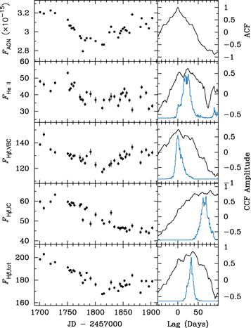
Figure 7. Light curves and CCF analysis results in 2019. The units and notations are the same as those in Figure 6. Note that the time lag of H could be underestimated here. See the text for a discussion.
Download figure:
Standard image High-resolution imageIn 2017, both He ii and H have negative values of measured time lags, with respect to the continuum at 5100 Å. The AGN continuum in this optical band has been observed to lag behind the ultraviolet (UV) continuum, which ionizes the line-emitting gas (e.g., Edelson et al. 2019). This is expected if the optical photons are emitted at a larger radius on the accretion disk than the UV photons (Cackett et al. 2007); the contribution of the diffuse continuum emission from BLR is also significant (Korista & Goad 2001; Lawther et al. 2018; Chelouche et al. 2019; Korista & Goad 2019; Netzer 2020). Considering the median sampling cadence of ∼4 days in this campaign and the uncertainties given by the CCCDs, the time lags of He ii and H
 are broadly consistent with zero, which means that their emitting-region sizes are comparable to the size of the part of the accretion disk that emits the optical continuum. The negative or nearly zero lags of He ii have been reported for many objects in previous reverberation mapping campaigns (e.g., Barth et al. 2013). But such a short lag of an Hβ component, containing ∼3/4 of the total fluxes, is totally surprising for such a luminous quasar (see Section 5.3 below for an estimation of the lag by the BLR radius–luminosity relation).
In 2019, H also had a slightly negative time lag consistent with zero, as in 2017. He ii showed a rather large time lag of
  days in 2019. However, the light curve of He ii showed a smaller variability amplitude but larger scattering than that in 2017, especially during the second half of the year. Thus, this change in the time lag of He ii between the two years has to be treated with caution, and this finding should be checked through future observations.
H showed significant lags of
  and
and  days (in the rest frame) in 2017 and 2019, respectively. If both H
 and H
and H are virialized, the lag of H
 can be estimated as τ(H
 ) ≈ τ(H
 ) × [FWHM(H
 )/FWHM(H
 )]2 ≈ 2.9 and 4.0 days in the two years, respectively. These values are consistent with our measurements of roughly zero, counting the potential time lag between the ionizing UV photons and the optical photons we observed. The measured time lag of H
 in 2019 was more than two times as long as that in 2017 (
 and
and  days, respectively). But both are roughly equal to the varying-flux-weighted (F × Fvar) average of the lags of H
 and H
and H in each year. Note that in 2017, the
  of H
of H was lower than those of both H
 and H
and H , indicating that such a decomposition in the dynamics of the BLR clouds is also valid in geometry.
Considering the little more than steady decline of the H light curve and the relatively short duration of the ∼200 days monitoring in 2019, the measured lag of ∼60 days for H
 could be underestimated. In addition, if this decline is not just the response to the dimming of the continuum in the first half of this season but contains a long-term trend in the variability of only the emission line, the measured time lag becomes much lower than the current value after subtracting a first-order polynomial to remove this trend (detrending; Welsh 1999). However, on a longer timescale, the light curves of the continuum and Hβ components of the entire 3 yr data set do not show different trends (Appendix A). Thus, we prefer to interpret the 2019 decline in the Hβ flux as due to reverberation of the varying continuum, and we choose not to apply detrending.
The large differences in both the velocities (as FWHMs) and the distances to the central continuum source (as lags) of the two broad Hβ components suggest that they are emitted from two separated regions. As mentioned in Section 1, direct modeling and velocity-resolved delays could be more convincing in identifying distinct emission-line components. In the next section, we show the results of velocity-resolved delays, but a direct modeling study is beyond of the scope of this paper.
4.3. Velocity-resolved Delays
As shown in Section 3, spectral fitting is better than simple integration for determining the continuum and decomposing the contaminations in this case. Thus, for obtaining the velocity-resolved delays of Hβ, we started with a broad-Hβ-only spectrum for each epoch after subtracting the best-fit models of all other spectral components.
17
Then, we generated the rms spectrum of the broad-Hβ-only spectra, and divided it into a dozen bins of equal fluxes between −6000 to 6000  in the velocity space.
18
The bottom panels of Figures 8 and 9 show the rms spectra (solid black histogram), and the boundaries of the velocity bins (dotted vertically lines) in years 2017 and 2019, respectively. Finally, light curves were measured by integrating the fluxes of the broad-Hβ-only spectra in each velocity-space bin, and time lags were obtained from the CCFs with the AGN continuum light curve given by the spectral fitting (in the left-top panels of Figures 6 and 7).
in the velocity space.
18
The bottom panels of Figures 8 and 9 show the rms spectra (solid black histogram), and the boundaries of the velocity bins (dotted vertically lines) in years 2017 and 2019, respectively. Finally, light curves were measured by integrating the fluxes of the broad-Hβ-only spectra in each velocity-space bin, and time lags were obtained from the CCFs with the AGN continuum light curve given by the spectral fitting (in the left-top panels of Figures 6 and 7).
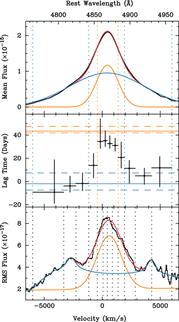
Figure 8. Top: the broad-Hβ-only mean spectrum (black) and the best-fit model (red) consist of H (blue) and H
 (orange). Middle: the velocity-resolved delays in the rest frame (dots with error bars). The horizontal solid lines mark the time lags of H
 (blue) and H
 (orange), and the associated dashed lines mark the 1σ errors. In the top and middle panels, the dotted blue and orange vertical lines divide the velocity bins into three groups: H
 only, H
 dominated, and mixed. Bottom: the broad-Hβ-only rms spectrum (black) and the best-fit model (red) consist of a Gaussian (orange) plus a disk profile (blue). The vertical dotted lines mark the boundaries of the bins of equal rms fluxes for measuring the velocity-resolved delays. Note that the measurements in the narrow velocity bins around the core are not independent due to the instrument broadening.
Download figure:
Standard image High-resolution image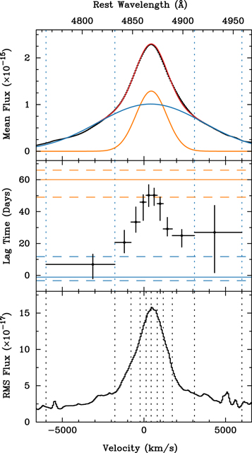
Figure 9. The broad-Hβ-only mean spectrum (top), the velocity-resolved delays (middle), and the broad-Hβ-only rms spectrum (bottom) in 2019. The notations are the same as those in Figure 8. Note that the measurements in the narrow velocity bins around the core are not independent due to the instrument broadening.
Download figure:
Standard image High-resolution imageFigures 10 and 11 show the light curves (black dots with error bars), and the corresponding CCFs (black curves) and CCCDs (blue histograms) for all of the velocity-space bins in 2017 and 2019, respectively. The velocity range of each bin (in units of kilometers per second) is written in the panel of each light curve. It increases from negative (blueshift) to positive (redshift) in a clockwise direction from bottom-left to bottom-right. As in Section 4.2, a systematic error (not shown in the figure) has been estimated and added before calculating the CCCD and the uncertainty of the lag. The time lags (in the rest frame) and their uncertainties for all of the bins are plotted at corresponding flux-weighted velocities in the middle panels of Figures 8 and 9. The error bars in the direction of the velocity mark the widths of the bins. The blue and orange horizontal solid lines show the lags of H and H
and H listed in Table 1, respectively. The associated horizontal dashed lines are 1σ error above and below. We also plot the broad-Hβ-only mean spectrum (black histogram) and the best-fit model (red curve), as the sum of H
 (the blue Gaussian) and H
 (the orange Gaussian), in the top panels of Figures 8 and 9.

Figure 10. Light curves (dots with error bars), CCFs (black lines), and CCCDs (blue histograms) for all of the velocity-space bins. The boundaries of each bin (in units of kilometers per second) are written in the panel of each light curve. From bottom-left to top-left, and then from top-right to bottom-right, the velocity increases from negative (blueshift) to positive (redshift).
Download figure:
Standard image High-resolution image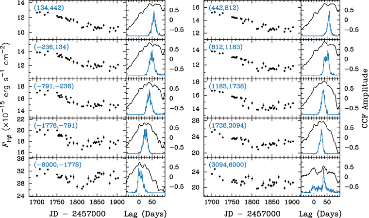
Figure 11. Light curves, CCFs, and CCCDs for all of the velocity-space bins in 2019. The notations are the same as those in Figure 10.
Download figure:
Standard image High-resolution imageIn 2017, the velocity-resolved delays were totally consistent with the two-component scenario. In the bluest and reddest three bins at the wings (between the two pairs of vertical blue dotted lines), the fluxes entirely come from H , and the lags are roughly equal to that of H
 . Note that the bluest bin could be contaminated by He ii while the reddest three bins could be influenced by Fe ii
λ4924, from the uncertainties in fitting the single-epoch spectra. On the other hand, for the four bins at the core (between the orange vertical dotted lines), the variabilities are dominated by that of H
. Note that the bluest bin could be contaminated by He ii while the reddest three bins could be influenced by Fe ii
λ4924, from the uncertainties in fitting the single-epoch spectra. On the other hand, for the four bins at the core (between the orange vertical dotted lines), the variabilities are dominated by that of H . The lags are roughly constant at ∼35 days, which is somewhat lower than the lag of H
 because of the mixture of H
 . For the other two bins at the transition between the wings and the core, the lags also transit from that at the wings to that at the core gradually as the fractions of H
 flux increase.
Three simple models with single kinematics are often used in the literature to understand the results of velocity-resolved delays: a virialized disk, an infall, and an outflow (see, e.g., Figure 10 in Bentz et al. 2009). However, the velocity-resolved delays of PG 0026+129 in 2017 cannot be interpreted by any single one of these models. A virialized disk shows shorter lags at the high-velocity wings, but not so discrete as we obtained here: those bins in the two wings have lags of nearly zero, while the lags of bins for the line core rise abruptly up to ∼35 days. The simplest interpretation is that there are two distinct regions: a compact one emitting H , plus another one much far away for H
 .
.
Another interesting result is the shape of the rms spectrum in 2017 shown in the bottom panel of Figure 8. It shows a complex profile with three peaks. When comparing with the mean spectrum (top panel), the core peak at the velocity of ∼300  matches H
 , and the other two peaks correspond to H
 . Without the core component, the wings of the rms spectrum show an asymmetric double-peaked profile with higher fluxes at the blue side. Such a profile has been observed in many AGNs, and is associated with a disk-like geometry (e.g., Storchi-Bergmann et al. 2017). See Section 5.4 below for more discussions.
In 2019, H had an
  approximately three times as large as that of H
 (see Table 1). The rms spectrum (Figure 9 bottom) is dominated by the variability in H
 , showing a strong core and weak wings, which is much different in shape compared to that in 2017. Due to the low fluxes at the wings in the rms spectrum, only the bluest and reddest bin correspond to the H
 -only region in the mean spectrum. The velocity-resolved delays (Figure 9 middle) still show a reliable lag consistent with that of H
 in the bluest bin, while the lag in the reddest bin is highly uncertain (the CCF in this bin has two peaks, see the bottom-right panel of Figure 11). A possible reason for this is the contamination by Fe ii
λ4924, which would be severe in the event of the weak H
in the bluest bin, while the lag in the reddest bin is highly uncertain (the CCF in this bin has two peaks, see the bottom-right panel of Figure 11). A possible reason for this is the contamination by Fe ii
λ4924, which would be severe in the event of the weak H variability seen here. For bins other than the reddest and bluest, the lags increase gradually toward the redshifted peak of the line, with increasing flux fraction of H
 . The velocity-resolved delays in 2019 are also consistent with the two-component scenario, although the pattern is not as discrete as that in 2017. The dominance of variability in H
 over that in H
 weakens the contrast between the lags at the wings and the core. See Section 5.3 below for more discussions on the much higher
  of H
of H in 2019.
5. Discussions
5.1. The Mass of the Central Black Hole
The virial mass of the central black hole can be estimated from the reverberation mapping measurements of the time lag τ and the emission-line width ΔV as

where c is the speed of light, G is the gravitational constant, and f is a virial factor counting for all other unknown effects including, e.g., the geometry and kinematics of the emitting region. In practice, f is obtained as an average for a sample of AGNs, by comparing the virial masses with those given by other methods, e.g., the MBH–σ* relation (Onken et al. 2004; Grier et al. 2013a). The AGNs are classified into subsamples according to, e.g., the properties of their bulges (Ho & Kim 2014), to reduce the uncertainty in the factor f. All of the calibrations of f in the literature are done for the time lags and the line widths measured from the total broad Hβ line.
The line width can be measured as either FWHM or line dispersion ( ), in either the mean or rms spectrum. See Peterson et al. (2004) for a thorough comparison of these methods. In principle, the rms spectrum is preferred for providing the varying part of the emission line for which the time lag is measured. But the rms spectrum usually has a much lower S/N than the mean spectrum, making the measurements more uncertain. In some cases, the rms spectrum shows emission lines too weak to measure (e.g., PG 2130+099 in 2018; Figure 2 of Hu et al. 2020), or dominated by other spectral components (e.g., the host galaxy, in MCG–6-30-15; Hu et al. 2016). The definition of FWHM is somewhat arbitrary, especially for those complex multiple-peaked profiles (our rms spectrum in 2017 as an example, bottom panel of Figure 8), while
  is well defined but sensitive to the subtraction of the underlying continuum. Thus, in order to alleviate the uncertainty introduced by the continuum subtraction and the contamination of He ii to the red wing of Hβ, we measure the FWHM and
  in the broad-Hβ-only mean and rms spectra, which are generated after subtracting all other components given by the spectral fitting, as for obtaining the velocity-resolved delays in Section 4.3. For FWHM, the method shown in Figure 1 of Peterson et al. (2004) is adopted. The uncertainties are given by the standard deviations of the values measured in Monte Carlo realizations (by bootstrap method) of the mean and rms spectra.
Table 3 gives the widths (Column 2) of the total broad Hβ measured by different methods (Column 1) in years 2017 and 2019. It can be seen that the shapes of the mean spectra in the two years are almost the same (compare the top panels of Figures 8 and 9). The changes in the widths presented by both FWHM and  are less than 5%. With a time lag in 2019 more than twice as long as that in 2017, the virial products (VPs; defined as cτ FWHM2/G or
  for FHWM or
  , respectively; Column 3) in 2019 are also more than twice as large. On the other hand, the shapes of the rms spectra change significantly between the two years, and thus the widths as well. Both FWHM and
  were much smaller in 2019, yielding more consistent VPs between the two years than by mean spectra. Particularly when FWHM in the rms spectrum is used, the difference in VPs between the two years is ≲15%. As mentioned in Section 4.2, the lag of H
 is roughly the varying-flux-weighted average of the H
 and H
and H lags. The large increase of H
 in 2019 accordingly strengthens H
 in the rms spectrum, and thus decreases the line width. The dramatic changes in the time lags and the rms spectra between the two years are both caused by the different behaviors of the two Hβ components. And the FWHM in the rms spectrum is preferred for line width measurements, as in this case it yields the most consistent VPs between the two years.
Table 3. Measurements for the Total Broad Hβ Line
| Method | Width | Virial Product | f |

|
|---|---|---|---|---|
( ) ) | (×107 M⊙) | (×107 M⊙) | ||
| (1) | (2) | (3) | (4) | (5) |
| 2017 | ||||
| Mean, FWHM | 3374 ± 27 |

| 1.3 |

|
Mean, 
| 2274 ± 4 |

| 5.6 |

|
| rms, FWHM | 2735 ± 578 |

| 1.5 |

|
rms, 
| 2446 ± 88 |

| 6.3 |

|
| 2019 | ||||
| Mean, FWHM | 3198 ± 21 |

| 1.3 |

|
Mean, 
| 2315 ± 4 |

| 5.6 |

|
| rms, FWHM | 1902 ± 114 |

| 1.5 |

|
rms, 
| 1901 ± 97 |

| 6.3 |

|
Note. Widths of the total broad Hβ line (Column 2) measured by different methods (Column 1) in years 2017 and 2019. The instrumental broadening has been corrected. Column (3) lists the virial products. Column (5) lists the masses of the central black hole estimated using the virial factors f (Column 4) corresponding to different width measurements given by Ho & Kim (2014). The uncertainty in f has not been included.
Download table as: ASCIITypeset image
Column (4) of Table 3 lists the virial factors f corresponding to different line width measurements from Ho & Kim (2014) for a classical bulge (see Ho & Kim 2014 for a discussion on the bulge type of PG 0026+129), and Column (5) lists the resultant black hole masses. Note that the masses given by  are several times higher than those given by FWHMs for the extremely small values of FWHM/
 of this target (see Figure 9 of Peterson 2014 for a comparison). Such a small FWHM/
 (∼1) in the rms spectra indicates that PG 0026+129 has wings much more variable than for most other objects. And the value of f in the table given as the mean in a sample is very probably unsuitable in this extreme case. The direct modeling method (Pancoast et al. 2011) could provide an estimate of the black hole mass without the assumption of f, but is out of the scope of this work. Therefore, considering that the masses given by the FWHMs in the rms spectra have the best consistency between the two years, we obtain the mass of the central black hole in PG 0026+129 as the weighted mean of the values given by this method:
  .
.
Previous estimations of the black hole mass of PG 0026+129 were based on the time lag measured by Kaspi et al. (2000), and were several times larger than the results here if the same method for line width measurement and f are used. For example, the VP given by  in the rms spectra remeasured by Peterson et al. (2004) is 7.14 ± 1.74 × 10⁷
M⊙, ∼4–5 times as large as our results by the same method. Possibly the time lag was overestimated in Kaspi et al. (2000) for undersampling (Grier et al. 2008), but there is no reliable black hole measurement by other methods for a comparison. The stellar velocity dispersion for PG 0026+129 has not been successfully measured in previous studies (Grier et al. 2013a), and the masses of its host galaxy or bulge are also largely uncertain. Ho & Kim (2014) gave a rather large bulge mass of
in the rms spectra remeasured by Peterson et al. (2004) is 7.14 ± 1.74 × 10⁷
M⊙, ∼4–5 times as large as our results by the same method. Possibly the time lag was overestimated in Kaspi et al. (2000) for undersampling (Grier et al. 2008), but there is no reliable black hole measurement by other methods for a comparison. The stellar velocity dispersion for PG 0026+129 has not been successfully measured in previous studies (Grier et al. 2013a), and the masses of its host galaxy or bulge are also largely uncertain. Ho & Kim (2014) gave a rather large bulge mass of  , based on the R-band magnitude. However, Bentz & Manne-Nicholas (2018) derived a much smaller mass of 1.7 × 10¹⁰
M⊙, by estimating the mass-to-light ratio using the V − H color. Using their Equation (3) for the
, based on the R-band magnitude. However, Bentz & Manne-Nicholas (2018) derived a much smaller mass of 1.7 × 10¹⁰
M⊙, by estimating the mass-to-light ratio using the V − H color. Using their Equation (3) for the  –Mbulge relation, the expected black hole mass is only 1.9 × 10⁷
M⊙. Better observations of the host galaxy, both multiband photometry and spectroscopy, are needed for a reliable bulge mass estimation.
–Mbulge relation, the expected black hole mass is only 1.9 × 10⁷
M⊙. Better observations of the host galaxy, both multiband photometry and spectroscopy, are needed for a reliable bulge mass estimation.
Comparing with the total Hβ line, H or H
or H can be potentially better for the virial mass estimation, because each of these components is hopefully less complex in geometry than the total line. The VPs given by the lag of H
 and its FWHM in the mean spectrum (see Table 1) were 3.27 × 10⁷ and 4.52 × 10⁷
M⊙ in years 2017 and 2019, respectively. These values are consistent with those given by the total line with the same method (FWHM in the mean spectrum), and the difference between the two years is smaller. The widths of the two components in the rms spectrum are presumably more suited for the mass estimation than the widths in the mean spectrum, as the former represents the varying part of each component. However, the decomposition of the two components in the rms spectrum is not so straightforward, due to its complex shape. On the other hand, the factor f for each single component is totally unknown so far.
and its FWHM in the mean spectrum (see Table 1) were 3.27 × 10⁷ and 4.52 × 10⁷
M⊙ in years 2017 and 2019, respectively. These values are consistent with those given by the total line with the same method (FWHM in the mean spectrum), and the difference between the two years is smaller. The widths of the two components in the rms spectrum are presumably more suited for the mass estimation than the widths in the mean spectrum, as the former represents the varying part of each component. However, the decomposition of the two components in the rms spectrum is not so straightforward, due to its complex shape. On the other hand, the factor f for each single component is totally unknown so far.
5.2. No Long-term Variation in the Broad Hβ Profile
As mentioned in Section 3.2, both H and H
and H are redshifted with respect to the narrow lines, by velocities of ≳400
  measured from the mean spectrum. Because of the relatively low spectral resolution of our spectra, it is not reliable to study the variations in the velocity shifts of the two components between different epochs during our campaign. But it is interesting to compare the Hβ profile in our spectra with those in Boroson & Green (1992) and Kaspi et al. (2000) for long-term variations in years.
PG 0026+129 was observed in 1990 October with better spectral resolution (∼360  ) by Boroson & Green (1992), and the spectrum is archived in the NED. As shown in Figure 12, we fit the Hβ line with three Gaussians: a narrow component (in orange) that is forced to have the same velocity shift and width as the [O iii] lines, and the other two Gaussians (in magenta) represent H
 and H
and H . The best-fit FWHMs (after instrumental broadening correction) and velocity shifts are ∼6710
  and ∼700
  for H
for H , and ∼1820
  and ∼340
  for H
for H , respectively. Note that the spectral shape of the archived spectrum is not well calibrated (the fluxes redward of the rest frame 5100 Å are lower than those of a power law extrapolated from the blueward part of the spectrum), so the measurements of broad Hβ components, especially H
 , are influenced by the uncertain continuum level. However, with their high spectral resolution, the Hβ profile of Boroson & Green (1992) clearly shows: (1) a narrow peak at zero velocity shift, indicating that the [O iii] lines are not blueshifted with respect to the low-ionizing narrow lines, and are thus appropriate for defining the systematic redshift of the object; (2) significant asymmetry, which is caused by the redshifted broad components, especially H
 .
.
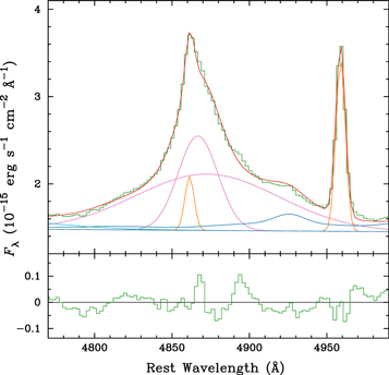
Figure 12. Fit of the archived spectrum in Boroson & Green (1992). The components involved in the fitting and the notations are the same as those in Figure 4. Note that their spectrum has higher spectral resolution and shows the asymmetry in the Hβ profile more clearly than our spectra.
Download figure:
Standard image High-resolution imageThe spectra in the Kaspi et al. (2000) campaign
19
also have low spectral resolution just comparable to that in this work (wide slits are usually used in reverberation mapping observations for good flux calibration). We generate mean spectra for the years 1993–1997, in which more than five epochs were observed. Figure 13 plots the mean spectra in these five years (green), along with the spectrum of Boroson & Green (1992) (red) and the mean spectra of the three years in our campaign (blue). The spectra are normalized by their flux at rest frame 5100 Å, and shifted vertically for clarity. The two vertical dashed lines mark the positions of Hβ λ4861 and [O iii] λ4959 with zero velocity shifts. See the widths of [O iii] λ4959 for a comparison of the spectral resolutions. For the spectra other than that of Boroson & Green (1992), the peaks of narrow Hβ lines are smoothed by the large instrumental broadening and can no longer be distinguished. But the redshifts of the broad line core, consisting of mainly H , are clear in all of the spectra. We decomposed the profiles and attempted to compare the velocity shifts of H
 between different years. No reliable variation was confirmed, presumably because of the uncertainty due to the unresolved narrow component.

Figure 13. Hβ profiles in different years from Boroson & Green (1992; in red), Kaspi et al. (2000; in green), and this work (in blue). The spectra are normalized and vertically shifted for clarity. The years when the spectra were observed are noted. The two vertical dashed lines mark the positions of zero shifts for Hβ λ4861 and [O iii] λ4959.
Download figure:
Standard image High-resolution imageIn summary, in view of the limited quality of the data, there is no evidence of significant change in the Hβ profile in these years. Most probably, the redshift of H remains roughly the same in nearly 30 yr.
5.3. Intermediate-width Component: An Infall?
The Fe ii emission lines of PG 0026+129 have similar widths to H , and are also redshifted, suggesting that both H
 and Fe ii are emitted from an intermediate-line region. Hu et al. (2008b) measured the velocity shifts of Fe ii emission in a large sample of quasars, and found that Fe ii are systematically redshifted (see Hu et al. 2012; Sulentic et al. 2012; Bon et al. 2018; Le & Woo 2019 for more discussions). The inverse correlation between the shift and the Eddington ratio in Hu et al. (2008b) indicates that these intermediate-width lines originate from an infall, because the radiation pressure increases with higher Eddington ratio and decelerates the infall more (Ferland et al. 2009). A similar inverse correlation between the velocity shift and the continuum flux should also exist in multi-epoch observations of a single object, as expected for an infall. However, as shown in Section 5.2, the current data allow for no such exploration.
The size of this intermediate-line region could be constrained by the time lags of H we measured in the two years, 43.4 and 60.0 light days, respectively. Adopting the mean fluxes of AGN continuum at 5100 Å given by our spectral fitting (2.74 × 10⁻¹⁵ erg s−1 cm−2 Å−1 in 2017 and 3.03 × 10⁻¹⁵ erg s−1 cm−2 Å−1 in 2019) and a luminosity distance
20
of 670 Mpc, we obtain spectral luminosities of λLλ
(5100 Å) = 7.5 × 1044 erg s−1 and 8.3 × 1044 erg s−1, respectively. Then the BLR radius–luminosity relation of Bentz et al. (2013) predicts radii of 98 and 104 lt-day, but for the whole Hβ line. Our measurement of H
we measured in the two years, 43.4 and 60.0 light days, respectively. Adopting the mean fluxes of AGN continuum at 5100 Å given by our spectral fitting (2.74 × 10⁻¹⁵ erg s−1 cm−2 Å−1 in 2017 and 3.03 × 10⁻¹⁵ erg s−1 cm−2 Å−1 in 2019) and a luminosity distance
20
of 670 Mpc, we obtain spectral luminosities of λLλ
(5100 Å) = 7.5 × 1044 erg s−1 and 8.3 × 1044 erg s−1, respectively. Then the BLR radius–luminosity relation of Bentz et al. (2013) predicts radii of 98 and 104 lt-day, but for the whole Hβ line. Our measurement of H is roughly half of the value predicted, and that of H
 is only one-eighth to one-fourth, by including the rather compact H
 . Note that shorter time lags than implied by that relation have been observed in many objects (Du et al. 2015; Grier et al. 2017). Especially for SEAMBH, time lags shortened by a factor of two are common and interpreted as a consequence of the self-shadowing effects (Wang et al. 2014; Du et al. 2018b). Adopting the black hole mass estimated in Section 5.1, the dimensionless accretion rates defined by Equation (2) in Du et al. (2015) have rather high values of 76 and 88, for the two years, indicating a SEAMBH in PG 0026+129. Thus, the small size of the intermediate-line region we measured is consistent with those in other SEAMBHs. However, such an extremely compact very-broad-line region that emits nearly three-fourths of the total fluxes has not been seen before, and most probably has a different origin.
The lag of H was ∼50% longer in 2019 than it was in 2017, while the AGN continuum was only 10% more luminous. In addition, H
 is much more variable (nearly 70% larger
  ) in 2019, while the variability amplitude of the continuum is mildly smaller. Another parameter worth noting here is the continuum variability timescale, which was apparently longer in 2019 (see the top panel of Figure 5). It is possible that the H
 region is more extended than what we measured here using time lags. As shown by the photoionization calculations and light-curve simulations in Goad & Korista (2014), the measured time lag and also the line responsivity will be reduced if the continuum varies faster than the maximum lag corresponding to the outer boundary of the emission-line region, because of the geometric dilution (see their Figure 9). Our results of the lags, variability amplitudes and timescales in the two years match this dilution effect qualitatively.
5.4. Very Broad Component: The Accretion Disk?
As shown in Section 4.3, the wings of the rms spectrum in 2017, corresponding to the velocity range of H , show an asymmetric double-peaked profile. But in the mean and single-epoch spectra, H
 is fitted well by a single Gaussian (see Figure 4 and the top panel of Figure 8). Different Hβ profiles in the mean and rms spectra are commonly seen in previous reverberation mapping campaigns, and interpreted as only a part of the total line fluxes that are variable to respond to the continuum variations (e.g., Peterson et al. 2004).
Double-peaked broad emission lines have been seen in many objects, including both low-luminosity AGNs (e.g., Ho et al. 2000; Shields et al. 2000; Bianchi et al. 2019) and Seyfert 1 galaxies (e.g., Storchi-Bergmann et al. 2017). The line is believed to be generated in the accretion disk itself (Strateva et al. 2003), or the inner part of the BLR, which is just the outward extension of the accretion disk (Storchi-Bergmann et al. 2017). The near-zero time lag between H and the optical continuum we measured in PG 0026+129 suggests that this very-broad-line region has to be tightly associated with the accretion disk. This very inner part of the BLR may just originate from the surface of the accretion disk, as suggested by some authors (e.g., Dumont & Collin-Souffrin 1990; Czerny & Hryniewicz 2011).
Following Bianchi et al. (2019), we fit the asymmetric double-peaked wings of the rms spectrum with the kerrdisk model developed by Brenneman & Reynolds (2006), which simulates the broad line emitted from an accretion disk system. The fitting is performed using xspec 12.10.1 (Arnaud 1996), and the results are shown in the bottom panel of Figure 8. The kerrdisk model is convolved with a Gaussian smoothing (in blue, after convolving), and an additional Gaussian line (in orange) is added as the intermediate-width component. The best fit (in red) constrains the parameters for the disk as follows: the emissivity index is  the inclination angle to the line of sight is
  and the inner and outer radii are
  and
and  , respectively, in units of gravitational radius defined as
  . The dimensionless spin of the black hole is not well constrained as
  , for the much larger inner radius than the marginally stable radius. Adopting MBH = 2.89 × 10⁷
M⊙ estimated in Section 5.1, the inner and outer radii are 0.25 and 2.29, in units of light days. For comparison, on a standard centrally illuminated thin accretion disk, the characteristic radius emitting at 5100 Å given by Equation (1) of Edelson et al. (2019) is 1.3 light days in the flux-weighted case, adopting an Eddington ratio of 1.9 in 2017 (by Lbol = 9λLλ
(5100 Å)). So the size of the disk given by modeling the double-peaked profile is consistent with the zero time lag of H
, for the much larger inner radius than the marginally stable radius. Adopting MBH = 2.89 × 10⁷
M⊙ estimated in Section 5.1, the inner and outer radii are 0.25 and 2.29, in units of light days. For comparison, on a standard centrally illuminated thin accretion disk, the characteristic radius emitting at 5100 Å given by Equation (1) of Edelson et al. (2019) is 1.3 light days in the flux-weighted case, adopting an Eddington ratio of 1.9 in 2017 (by Lbol = 9λLλ
(5100 Å)). So the size of the disk given by modeling the double-peaked profile is consistent with the zero time lag of H we measured, supporting the accretion disk origin of the very broad component.
On the other hand, the diffuse continuum emission from the line-emitting clouds is unavoidable and contributes rather significantly to the observed optical continuum in the calculations of several models of the BLR (e.g., Korista & Goad 2001; Chelouche et al. 2019; Netzer 2020). Thus the time lag of the optical continuum with respect to the UV continuum could be longer than that given by the illuminated disk model by a factor of a few times for the contribution of this non-disk continuum (e.g., Lawther et al. 2018; Chelouche et al. 2019; Korista & Goad 2019). In this case, the variations in the H emission from the disk fitted above will lead those of the 5100 Å continuum by a few days. However, the quality of our data set, mainly the sampling interval, does not allow for reliable determination of negative lags of a few days. Interestingly, in the model of Chelouche et al. (2019), the non-disk continuum emission is emitted by the gas launched from the accretion disk, which may correspond to the region responsible for H
 in terms of size, although in their model, high gas density suppressed Balmer lines by collisional de-excitation (Baskin et al. 2014).
The photoionized accretion disk model in Dumont & Collin-Souffrin (1990) produces copious Balmer lines but collisionally suppressed Lyα (Rokaki et al. 1992), as observed in Arp 102B. The double-peaked components are strong in Balmer lines, and can be fitted by a disk with similar size in units of gravitational radius (Halpern et al. 1996) as that given for PG 0026+129 above. But Lyα shows no such disk component in Arp 102B (Figure 3 of Halpern et al. 1996). By contrast, the profile of the Lyα line in PG 0026+129 (see Hubble Space Telescope/Faint Object Spectrograph spectrum collected by Bechtold et al. 2002) shows strong wings, even broader than H , indicating that the collisional de-excitations are not dominant in the H
 -emitting clouds in PG 0026+129. Detailed photoionization modeling, which is beyond the scope of this paper, may reveal why PG 0026+129 is unique (so far) in having such strong line emission emitted so close to the ionizing source.
In 2019, while the mean spectrum retained the same strong H , the rms spectrum showed no double-peaked wings as clearly as in 2017, a result of the more variable H
 . But relatively weak, very broad wings are evident. Thus, the rare existences of outstanding H
 in both the velocity-resolved delays and the rms spectrum in the literature do not necessarily mean that such an H
 is unique for PG 0026+129. It is possible that compact disk-like H
 also exist in other AGNs, but not as strong and variable as that of PG 0026+129 in 2017, or they just hide beneath the other more variable parts of the BLR, as in the case of 2019 here. High-quality velocity-resolved delay measurements would hopefully reveal this kind of H
 in more AGNs, with fast driving continuum variations.
6. Summary
We performed a new reverberation mapping campaign of the quasar PG 0026+129 using the CAHA 2.2 m telescope lasting three years from 2017 to 2019. In the first and third years, the object had sizable variations in the continuum fluxes, and significant reverberations of broad He ii and Hβ emission lines were detected. The spectral decomposition and time-series analysis showed strong evidence that two kinematically and geometrically distinct Hβ-emitting regions exist. The main results can be summarized as follows:
- 1.The broad Hβ emission line can be decomposed into two components: a very broad H
 with an FWHM of 7570 ± 83 , and another intermediate-width H with an FWHM of 1964 ± 18 . Both components show significant reverberations to the continuum variations. The time lags (in the rest frame) are and days for H, and days for H, in 2017 and 2019, respectively.
 - 2.The velocity-resolved delays are roughly zero at the Hβ wings and ∼30–50 days at the core, with no gradual transition between these regimes, supporting the existence of two distinct broad Hβ components.
- 3.H and Fe ii emission have similar line widths, and both are redshifted, indicating that they both originate from an intermediate-width line region, which could be an infall.
- 4.In 2017, a reliable lag of days for the broad He ii line was also detected. H and He ii have similar line widths and time lags. We suggest that both of them are emitted from a region associated with the accretion disk, because: (1) the lags of close to zero indicate that the region has a size comparable to that of the part of the accretion disk emitting the optical continuum; (2) the rms spectrum of H shows an asymmetric double-peaked profile, which suggests a disk-like structure.
- 5.Combining the time lags for the total Hβ broad line and the FWHMs in the rms spectra yields the mass of the central black hole with the best consistency between the two years. The weighted mean is adopted, assuming a virial factor of 1.5.


We acknowledge the support of the staff of the CAHA 2.2 m telescope. This work is based on observations collected at the Centro Astronómico Hispanoen Andalucía (CAHA) at Calar Alto, operated jointly by the Andalusian Universities and the Instituto de Astrofísica de Andalucía (CSIC). This research is supported by the National Key R&D Program of China (2016YFA0400701, 2016YFA0400702), by the National Science Foundation of China (11721303, 11773029, 11833008, 11873048, 11922304, 11973029, 11991051, 11991052, 11991054, 12003036, 12022301), by the Key Research Program of Frontier Sciences of the Chinese Academy of Sciences (CAS; QYZDJ-SSW-SLH007), by the CAS Key Research Program (KJZDEW-M06), and by the Strategic Priority Research Program of the CAS (XDB23000000, XDB23010400). J.A. acknowledges financial support from the State Agency for Research of the Spanish MCIU through the "Center of Excellence Severo Ochoa" award to the Instituto de Astrofísica de Andalucía (SEV-2017-0709).
Appendix A: Results from the Entire Data Set of Three Years
This appendix presents the results of the time-series analysis performed on the entire data set of the three years. In general, the time lags measured from data sets with multiple observing seasons should be treated with caution, because of the gaps between the observing seasons and possible different long-term trends in the light curves. For comparison, the javelin software (Zu et al. 2011) was also used for the 3 yr data set. By assuming a damped-random-walk model and a top-hat transfer function, javelin treats the seasonal gaps in a more sophisticated manner than ICCF. The results from javelin and ICCF are generally consistent, and the numbers listed below are given by ICCF.
Figure 14 shows the light curves, CCFs, CCCDs, and the javelin posterior distributions of lags for the broad emission lines and components. The time lags are  and
and  days in the rest frame for H
 and H
and H , respectively. For the total Hβ, the measured time lag is
  days. The light curves of the two Hβ components and the total Hβ show no obvious long-term trend differing from the AGN continuum.

Figure 14. Light curves and CCF analysis results for the entire three years. The units and notations are the same as those in Figure 6, while the additional orange histograms are the javelin posterior distributions of the lags.
Download figure:
Standard image High-resolution imageFigure 15 shows the broad-Hβ-only mean spectrum and the decomposition, the velocity-resolved delays, and the rms spectrum. Figure 16 shows the light curves, CCF analysis, and javelin posterior distributions for each velocity bin. The differences between the lags from ICCF and javelin in the bluest two bins indicate the measurements in these bins have large uncertainties as in the 1 yr data set mentioned in Section 4.3, which may be influenced by the inaccurate decomposition of Fe ii
λ4924 in the spectral fitting. The velocity-resolved delays show an obvious discrete structure consistent with the two-component scenario: the lags in wing bins equal that of H , while the lags in the core bins jump up close to that of H
 .
.

Figure 15. The broad-Hβ-only mean spectrum (top), the velocity-resolved delays (middle), and the broad-Hβ-only rms spectrum (bottom) for the entire three years. The notations are the same as those in Figure 8. Note that the measurements in the narrow velocity bins around the core are not independent due to the instrument broadening.
Download figure:
Standard image High-resolution image
Figure 16. Light curves, CCFs, and CCCDs for all of the velocity-space bins for the entire three years. The notations are the same as those in Figure 10, while the additional orange histograms are the javelin posterior distributions of the lags.
Download figure:
Standard image High-resolution imageAppendix B: Spectra Obtained with the Sutherland 1.9 m Telescope
During the campaign, PG 0026+129 was also observed by the Sutherland 1.9 m telescope at the South African Astronomical Observatory. Spectra were taken with the 600 lines mm−1 grating and 40 slit for several epochs (see Winkler & Paul 2017 and also Hu et al. 2020 for more details on the observations and data reduction). The spectral resolution is ∼340  estimated by the FWHM of the sky line, better than that of our CAHA spectra. In addition, [O ii] λ3727 is covered. Thus, we present a Sutherland spectrum here to investigate whether [O iii] is blueshifted with respect to the low-ionization lines.
Figure 17 shows a spectrum taken on JD 2458322 in 2018 July. It is well fitted by the same spectral components described in Section 3.2. The FWHMs (after instrumental broadening correction) and the velocity shifts (with respect to [O iii]) are 7225  and 449
  for H
for H , and 1847
  and 403
  for H
for H , respectively. [O ii] λ3727 is clearly detected as shown in the inserted plot. A simple fit to the doublet with a single Gaussian above a locally defined continuum yields a blueshift of 48
  with respect to the [O iii] lines. The uncertainty in the measurement of the [O ii] shift introduced by the unknown line ratio of the doublet has to be smaller than the pair separation (2.78 Å or 224
  ). Thus, the ≳400
  redshifts of the two broad Hβ components cannot be interpreted as [O iii] being blueshifted in this object. In addition, the peak of the Hβ profile is well fitted by the narrow Hβ component, which is forced to have the same velocity width and shift as those of [O iii], supporting that [O iii] is not blueshifted and is appropriate for defining the systematic redshift of this object.
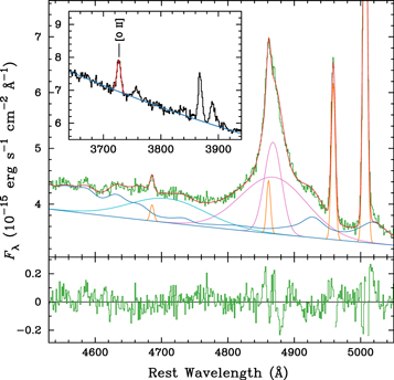
Figure 17. Fit of a spectrum obtained with the Sutherland 1.9 m telescope on JD 2458322. The spectrum has been de-redshifted according to the [O iii] lines. The components involved in the fitting and the notations are the same as those in Figures 4 and 12. The inserted plot shows the fit by a Gaussian (red) above a local continuum (blue) to [O ii] λ3727, whose position of zero velocity shift is marked. Note that the [O iii] lines are not blueshifted with respect to either the Hβ peak or [O ii].
Download figure:
Standard image High-resolution imageFootnotes
- 13
Note that the terms "intermediate-width component" and "very broad component" have been used in the literature for different emission lines including not only Hβ but also Mg ii, C iv, etc. (e.g., Brotherton et al. 1994; Sulentic & Marziani 1999; Popović et al. 2019). In this paper, they refer to the Hβ emission line only.
- 14
This value is given by the shift of the [O iii] λ5007 line in our spectra, and is slightly larger than that in the NASA/IPAC Extragalactic Database (NED; http://ned.ipac.caltech.edu/). See Sections 3.2 for details.
- 15
IRAF is distributed by the National Optical Astronomy Observatories, which are operated by the Association of Universities for Research in Astronomy, Inc., under cooperative agreement with the National Science Foundation.
- 16
Except those for H
. They are the mean FWHMs of the individual-night spectra measured from the best-fit models, in each year. The errors are the standard deviations. - 17
We also generated the velocity-resolved light curves by the traditional integration from the original spectra. The yielded velocity-resolved delays show similar features as those given by the broad-Hβ-only spectra here: zero lags at the wings and long lags at the core, although the uncertainties are larger.
- 18
The velocity binning around the line core is below the instrumental resolution of ∼1000
, and thus the measurements near the line core are not independent. - 19
- 20
Based on z = 0.1454 and cosmological parameters of H0 = 72 km s−1 Mpc−1, Ωm = 0.3, and ΩΛ = 0.7.

