


Abstract
Supernova (SN) 2017cbv in NGC 5643 is one of a handful of Type Ia supernovae (SNe Ia) reported to have excess blue emission at early times. This paper presents extensive BVRIYJHKs-band light curves of SN 2017cbv, covering the phase from −16 to +125 days relative to B-band maximum light. The SN 2017cbv reached a B-band maximum of 11.710 ± 0.006 mag, with a postmaximum magnitude decline of Δm15(B) = 0.990 ± 0.013 mag. The SN suffered no host reddening based on Phillips intrinsic color, the Lira–Phillips relation, and the CMAGIC diagram. By employing the CMAGIC distance modulus μ = 30.58 ± 0.05 mag and assuming H0 = 72 km s−1 Mpc−1, we found that 0.73 M⊙ 56Ni was synthesized during the explosion of SN 2017cbv, which is consistent with estimates using reddening- and distance-free methods via the phases of the secondary maximum of the near-IR- (NIR-) band light curves. We also present 14 NIR spectra from −18 to +49 days relative to the B-band maximum light, providing constraints on the amount of swept-up hydrogen from the companion star in the context of the single degenerate progenitor scenario. No Paβ emission feature was detected from our postmaximum NIR spectra, placing a hydrogen mass upper limit of 0.1 M⊙. The overall optical/NIR photometric and NIR spectral evolution of SN 2017cbv is similar to that of a normal SN Ia, even though its early evolution is marked by a flux excess not seen in most other well-observed normal SNe Ia. We also compare the exquisite light curves of SN 2017cbv with some Mch delayed detonation models and sub-Mch double detonation models.
Export citation and abstract BibTeX RIS
1. Introduction
Type Ia supernovae (SNe Ia) have served as cosmological distance indicators for the past three decades and led to the discovery of the accelerating expansion of the universe (Riess et al. 1998; Perlmutter et al. 1999). After corrections for the light-curve/color parameters (i.e., Δm15; Phillips 1993; Riess et al. 1996; Tripp 1998; Guy et al. 2005; Wang 2005), the magnitude dispersion on the Hubble diagram of SNe Ia can be brought down to below 0.1 mag rms (e.g., Wang 2005; Wang et al. 2009a; Burns et al. 2018; He et al. 2018). Increasing evidence suggests that near-IR (NIR) light curves of SNe Ia are better standard candles (Phillips 2012; Avelino et al. 2019) and intrinsically less affected by dust extinction from the host galaxy (Meikle 2000; Krisciunas et al. 2004a, 2004b, 2007). The scatter in the NIR Hubble diagram can reach 0.15 mag without applying any light-curve/color parameter corrections (Krisciunas et al. 2004a; Wood-Vasey et al. 2008; Folatelli et al. 2010).
There is a general consensus that SNe Ia are the thermonuclear explosion of carbon–oxygen white dwarfs (WDs), and many of them seem to explode near the Chandrasekhar mass (Mch; Hillebrandt & Niemeyer 2000), although they may originate from progenitors of other masses as well (Scalzo et al. 2014b). There are two popular progenitor scenarios, the single degenerate (SD) and the double degenerate (DD); see recent reviews by Wang & Han (2012), Maoz et al. (2014), and Jha et al. (2019). In the SD model, a carbon–oxygen WD accretes material from a nondegenerate companion star such as a red giant, subgiant, main-sequence, or helium star (Whelan & Iben 1973; Livne 1990; Woosley & Weaver 1994; Nomoto et al. 1997), while in the DD model, the system comprises two WDs (Iben & Tutukov 1984; Webbink 1984).
A very clear sign of the SD model lies in the very early light curves, when a "blue bump" may appear in the near-UV (NUV)–optical bands as a result of the collision of SN ejecta with the nondegenerate companion (Kasen 2010; Marion et al. 2016). Excess emission in the early light curve has been reported in a number of SNe Ia (Cao et al. 2015; Marion et al. 2016; Hosseinzadeh et al. 2017c; Jiang et al. 2018; Dimitriadis et al. 2019a; Li et al. 2019b; Shappee et al. 2019). Alternatively, these early light-curve features may be associated with mixing of radioactive 56Ni (Jiang et al. 2020; Magee et al. 2018, 2020; Magee & Maguire 2020; Miller et al. 2018; Piro & Morozova 2016), He shell detonation (Jiang et al. 2017; Maeda et al. 2018; Polin et al. 2019; Siebert et al. 2020), or circumstellar material interaction in the DD scenario (Levanon & Soker 2017, 2019). Meanwhile, other studies have searched for narrow Hα/He emission lines in nebular phase spectra as a characteristic signature of the SD scenario (Marietta et al. 2000; Mattila et al. 2005; Leonard 2007; Pan et al. 2010, 2012; Liu et al. 2012, 2013; Lundqvist et al. 2013; Graham et al. 2015; Lundqvist et al. 2015; Maguire et al. 2016; Botyánszki et al. 2018; Sand et al. 2018, 2019; Shappee et al. 2018, 2018; Dimitriadis et al. 2019b; Holmbo et al. 2019; Tucker et al. 2019). However, no definitive late-time narrow emission features of hydrogen (i.e., Hα) have been detected among current samples of normal SNe Ia. Recent observations for fast-declining, subluminous SNe Ia have detected narrow Hα emission in two cases, SNe 2018fhw (Kollmeier et al. 2019) and 2018cqj (Prieto et al. 2020). The Hα luminosity could be due to stripped hydrogen from a nondegenerate companion in the SD progenitor scenario (Kollmeier et al. 2019; Prieto et al. 2020). Or it could originate from ejecta–circumstellar medium (CSM) interaction (Kollmeier et al. 2019; Vallely et al. 2019; Dessart et al. 2020), a scenario similar to luminous Type Ia CSM objects (Hamuy 2003; Wang et al. 2004; Aldering et al. 2006; Prieto et al. 2007; Dilday et al. 2012; Silverman et al. 2013; Graham et al. 2019).
Additionally, recent observational and theoretical studies of SNe Ia have shown that the NIR spectra have several key physical diagnostics capable of discriminating potential progenitor systems and explosion mechanisms (Ashall et al. 2019a, 2019b; Hsiao et al. 2019). Unburned carbon C i λ1.069 μm can be used to probe the primordial material directly from the progenitor (Hsiao et al. 2013, 2015). Its abundance and distribution in the ejecta also provide strong constraints on explosion models. For instance, the turbulent and pure deflagration models predict a large amount of unburned carbon (Gamezo et al. 2003; Kozma et al. 2005). In contrast, the delayed detonation (DDT) models predict nearly complete carbon burning (Kasen et al. 2009). On the other hand, substantial unburned carbon is not expected to survive in the explosions of sub-Chandrasekhar-mass WDs through the double detonation mechanism (Fink et al. 2010). Furthermore, narrow Paβ λ1.282 μm emission is expected in the SD scenario (for a red giant companion) 1–2 months after maximum light (Maeda et al. 2014). Searching for such emission has only been undertaken in a handful of objects but is another promising signature of the SD scenario (e.g., Sand et al. 2016).
The SN 2017cbv (DLT17u) gained much attention because it shows a very clear "blue bump" as reported by Hosseinzadeh et al. (2017c). Narrow emission lines H/He have not been detected in the nebular phase spectra (Sand et al. 2018), and time-variable narrow-line features of Na i D and Ca ii H&K have not been detected within high-resolution spectra (Ferretti et al. 2017). These observational signatures, together with the fact that SN 2017cbv was discovered so young, make it an interesting target to study with respect to its progenitor system and explosion physics.
Here we present extensive optical and NIR observations of SN 2017cbv, including BVRIYJHKs-band photometry lasting 140 days, using the same instrument and 14 NIR spectra. In Section 2, we describe the observational data and data analyses of SN 2017cbv. In Section 3, we present the physical properties of SN 2017cbv from our well-sampled light curves, including our light/color curves, color–magnitude diagrams (CMDs), host reddening and its distance determination, and bolometric light curves. In Section 4, we present theoretical perspectives of SN 2017cbv. We summarize our results in Section 5.
2. Data and Data Analyses
Our data include optical/NIR photometry from −16 to +125 days and 14 NIR spectra from −18 to +49 days after B-band maximum, making SN 2017cbv one of the earliest NIR spectra ever taken for SNe Ia. The SN 2017cbv was discovered on 2017 March 10.14 (UT dates are used throughout this paper) by the D < 40 Mpc survey (DLT40; Tartaglia et al. 2018; Yang et al. 2019), and a confirmation image was obtained with the same telescope 30 minutes later (Tartaglia et al. 2017). It has coordinates α = 14h32m34 42 and δ = −44°08'02
 8 (J2000.0). It is located 68'' west and 145'' north of the center of galaxy NGC 5643, which has an SAB(rs)c morphology (de Vaucouleurs et al. 1991) and a Tully–Fisher distance modulus of 31.14 ± 0.40 mag (Tully & Fisher 1988). The SN Ia 2013aa also exploded in this galaxy (Parker et al. 2013; Parrent et al. 2013), and a comprehensive comparison between SNe 2017cbv and 2013aa is described in Burns et al. (2020). A spectrum of SN 2017cbv was acquired shortly after its discovery, showing it to be a very young SN Ia with high-velocity features similar to those of SN 1999aa at t > 2 weeks before maximum light (Hosseinzadeh et al. 2017a, 2017b).
Our photometric observations of SN 2017cbv started on 2017 March 13.17, ∼16 days before B-band maximum. Data were collected in the BVRIYJHKs bands with the CTIO 1.3 m telescope and dual-channel optical/NIR camera ANDICam. This instrument has an optical field of view (FOV) of 6 3 × 63 (037 pixel−1) and an NIR FOV of 24 × 24 (027 pixel−1).
The first NIR spectrum of SN 2017cbv was taken with FLAMINGOS-2 (Eikenberry et al. 2006) on the Gemini South 8.2 m telescope at only 2.30 days past the explosion, representing one of the earliest NIR spectra ever taken for an SN Ia. Similar early-phase NIR spectra were only obtained for SN 2011fe (Hsiao et al. 2013) and iPTF13ebh (Hsiao et al. 2015). Five more NIR spectra were also obtained with FLAMINGOS-2, covering the phase from −18 to +36 days from B-band maximum light. Two other spectra were provided by ePESSTO (Smartt et al. 2015) with the SOFI instrument (Moorwood et al. 1998) on the New Technology Telescope (NTT). Five NIR spectra were also acquired with FIRE (Simcoe et al. 2013) on the Magellan Baade telescope. One more spectrum was taken with the SpeX spectrograph (Rayner et al. 2003) on the NASA Infrared Telescope Facility (IRTF). A journal of the NIR spectroscopic observations is shown in Table 1.
Table 1. Log of the NIR Spectroscopic Observations
| UT Date | MJD |

|
Instrument | texp | Airmass |
|---|---|---|---|---|---|
| (s) | |||||
| 2017-03-11 | 57,823.30 | −17.57 | FLAMINGOS-2 | 8 × 150 | 1.03 |
| 2017-03-13 | 57,825.30 | −15.57 | FLAMINGOS-2 | 8 × 150 | 1.04 |
| 2017-03-17 | 57,829.40 | −11.47 | FLAMINGOS-2 | 8 × 60 | 1.03 |
| 2017-03-22 | 57,834.30 | −6.57 | FLAMINGOS-2 | 8 × 20 | 1.08 |
| 2017-03-26 | 57,838.25 | −2.62 | FIRE | 8 × 126.8 | 1.06 |
| 2017-04-02 | 57,845.30 | 4.43 | FLAMINGOS-2 | 8 × 15 | 1.06 |
| 2017-04-14 | 57,857.14 | 16.27 | FIRE | 8 × 126.8 | 1.16 |
| 2017-04-21 | 57,864.27 | 23.40 | FIRE | 4 × 126.8 | 1.08 |
| 2017-04-23 | 57,866.20 | 25.33 | SOFI | 4 × 50 | 1.04 |
| 2017-05-02 | 57,875.27 | 34.40 | FIRE | 4 × 126.8 | 1.14 |
| 2017-05-04 | 57,877.20 | 36.33 | FLAMINGOS-2 | 8 × 25 | 1.05 |
| 2017-05-04 | 57,877.37 | 36.50 | SpeX | 10 × 150 | 2.47 |
| 2017-05-17 | 57,890.22 | 49.35 | FIRE | 4 × 126.8 | 1.12 |
| 2017-05-17 | 57,890.24 | 49.37 | SOFI | 4 × 50 | 1.16 |
Note.  : relative to the epoch of B-band maximum,
  = 57,840.87 MJD from GPR (Rasmussen 2006; Pedregosa et al. 2011).
Download table as: ASCIITypeset image
2.1. Optical Photometry
2.1.1. Data Reduction and Astrometry
The raw optical images were collected by the Yale SMARTS team and reduced through a data pipeline via the NOAO IRAF package.26 The reduction included the subtraction of an overscan region, a zero frame, and division by a normalized dome flat.27 The reduced images were downloaded from the SMARTS ftp site. Then, cosmic rays were detected and removed using Laplacian cosmic-ray identification (van Dokkum 2001).28 The astrometric calibration for the optical images were carried out using Astrometry.net (Lang et al. 2010).
2.1.2. Differential Photometry
As SN 2017cbv is located far away (160'') from the center of its host galaxy, light contamination from the host is negligible (see Figure 1). Aperture and point-spread function (PSF) photometry were performed on the optical images of SN 2017cbv.
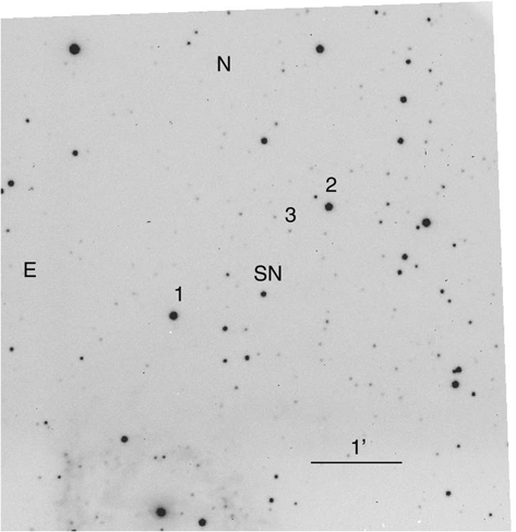
Figure 1. The SN 2017cbv in NGC 5643. This is a B-band image taken with the CTIO 1.3 m on 2017 July 31.99. The SN 2017cbv and three local reference stars (Tables 3 and 4) for BVRIYJHKs calibration are marked by numbers. Star 2 was used for optical calibration, and star 1 was used for NIR calibration.
Download figure:
Standard image High-resolution imageThe photometry of the stars in the field was not completely consistent when comparing Carnegie Supernova Project (CSP; Burns et al. 2020) and ANDICam images. We found an uncorrected illumination pattern in the ANDICam images, which is more evident when combining a large number of images. Unfortunately, there are no available flat-field images to make a proper correction, so instead, we opted to use only stars in the neighborhood of the SN to produce relative photometry. In detail, we used two bright and isolated stars in the close neighborhood of SN 2017cbv to measure differential photometry (we did not detect time-series variability for the two selected stars during our observing window). The CSP also observed the field in the ugriBV bands (Burns et al. 2020) and provided us with their calibration in order to derive the BVRI values. We measured differential photometry using PSF and aperture photometry relative to star 2 (using the PSFEx and SEP tools, respectively; Bertin & Arnouts 1996; Bertin 2011; Barbary 2018), as star 1 was saturated in all CSP ri-band images but not on our ANDICam images. We used the PSF photometry, as it was also used in the NIR images. We took the aperture photometry as a sanity check, showing a 0.02 mag systematic deviation, which was added to the final error budget as a systematic error.
2.1.3. Calibration of the Local-sequence Stars
Due to the illumination problem (see above), we did not calibrate the stars in the SN field; instead, we used calibrations from CSP photometry (Burns et al. 2020). The BV-band calibrations of ANDICam in the natural system were transformed from CSP BV bands via its color term coefficients of B − V in Table 2. The ANDICam R- and I-band calibrations in the natural system were derived in a similar way, and the standard magnitudes of the CSP RI bands were measured from the average values of the ri bands following the Sloan Digital Sky Survey (SDSS) transformation equations (Jester et al. 2005; Lupton et al. 2005; Jordi et al. 2006). The BVRI magnitudes of star 2 are listed in Table 3.
Table 2. Transformation Coefficients of Color Terms in the BVRI Bands
| Filter | Color Term C | Extinction Coefficient K |
|---|---|---|
| B | 0.059 ± 0.014 | 0.251 |
| V | −0.041 ± 0.007 | 0.149 |
| R | −0.015 ± 0.027 | 0.098 |
| I | −0.079 ± 0.015 | 0.066 |
Download table as: ASCIITypeset image
Table 3. Magnitudes of the Optical Photometry Sequence for SN 2017cbv
| Star | R.A. | Decl. | B | V | R | I |
|---|---|---|---|---|---|---|
| (J2000.0) | (J2000.0) | |||||
| 2 | 14:32:30.4 | −44:07:04.6 | 14.378 ± 0.013 | 13.876 ± 0.011 | 13.546 ± 0.023 | 13.260 ± 0.014 |
Note. Units of R.A. are hours, minutes, and seconds, and units of decl. are degrees, arcminutes, and arcseconds. See Figure 1 for a chart of SN 2017cbv.
Download table as: ASCIITypeset image
2.1.4. Optical Color Terms
In spite of having a calibrated set of local-sequence stars, we still need color terms to transform instrumental photometry into the standard system. The color terms of ANDICam were determined from images of the standard field Rubin 149 following the equations


where bvri are the instrumental magnitudes; BVRI are the standard magnitudes; ZB, ZV, ZR, and ZI are the zero-point magnitudes; kB, kV, kR, and kI are the extinction coefficients; X is the airmass; and CB, CV, CR, and CI are the color terms. We adopted the same extinction coefficients from CTIO's calibration pages in Table 2. The Rubin 149 field was observed for 60 photometric nights, and the color term parameters in Table 2 were determined by calibrating the Landolt standard stars in Rubin 149.
2.1.5. Comparison with Other Photometric Observations
We compared the BVRI-band photometry of SN 2017cbv observed with ANDICam to the data of Wee et al. (2018), the CSP II program (Burns et al. 2020), and the 1 m data taken with the Las Cumbres Observatory Supernova Key Project and Global Supernova Project (Hosseinzadeh et al. 2017c); see Figure 2. Our BV-band photometry is consistent with CSP II and Hosseinzadeh et al. (2017c) within 0.05 mag, while our BVRI-band light curves are systematically fainter by 0.101 ± 0.042, 0.156 ± 0.027, 0.108 ± 0.018, and 0.152 ± 0.023 mag relative to the same filter in Wee et al. (2018). We double-checked our photometry by employing two independent methods simultaneously (aperture and PSF photometry), while only aperture photometry was used in Wee et al. (2018). Our aperture photometry is corrected by the aperture size. The aperture correction was measured on bright isolated stars between 15'' and 7'' and applied to 7'' aperture photometry. This is the same method used to measure standard stars by Landolt (2009). Our calibration involved independent observations of local-sequence stars taken from the CSP II project, while Wee et al. (2018) took observations of standard star fields for calibration and target fields with the same instrument. Our BV-band photometry is most consistent with that from CSP II (Burns et al. 2020) and Hosseinzadeh et al. (2017c).

Figure 2. Comparison of BVRI-band light curves of SN 2017cbv between ANDICam (this work), Wee et al. (2018), the CSP II program (Burns et al. 2020), and the Las Cumbres Observatory's 1 m telescope (Hosseinzadeh et al. 2017c). The bottom four panels show the differences between ANDICam and other surveys in the BVRI bands.
Download figure:
Standard image High-resolution image2.2. NIR Photometry
2.2.1. Data Reduction and Astrometry
The ANDICam NIR raw images have been binned on-site at CTIO using an IRAF script and uploaded to the Yale Repository. For the binned NIR images, we first applied flat-field correction and cosmic-ray rejection. Then, a sky frame was subtracted from each image using neighboring images; if the three dithered science images (a, b, and c) were taken one by one with the same exposure time, the differences of two neighboring images (a-b, b-a, and c-b) were taken as the sky-subtracted images. We measured the dither offsets relative to the first frame by picking up a bright source on the dithered science images using skycat29 and took the measured dither offsets as the initial values for all science frames. Stars were extracted on the image after the initial dither offset correction (Bertin & Arnouts 1996), and their pixel positions were matched to get additional shifts. The images with corrections for the dither offset- (initial + extra) corrected frames were then combined to create a coadded image, which can be used to perform photometry simultaneously via source extraction and photometry (SEP; Barbary 2018) and the PSF Extractor (PSFEx; Bertin & Arnouts 1996; Bertin 2011) after astrometric calibration. For the NIR images, WCS information was added manually to one reference image, and then all other images were aligned with the reference using the Python module Astroalign (Beroiz et al. 2020).
2.2.2. Differential Photometry
As we did for the optical images, we performed differential photometry of SN 2017cbv relative to neighbor stars 1 and 3 (∼3 mag fainter than 1; see Figure 1). We did not take star 2 as the local star because it is too close to the image's edge. We found that PSF photometry performs better than aperture photometry. We tested this by comparing the variance of the difference between stars 1 and 3, which is smaller for the PSF than aperture photometry in all filters. We also noted an intrinsic dispersion of the order of 0.025 mag for the PSF difference distribution, which we account for as an instrumental noise component, and add it to the photometry error budget. As star 1 is brighter and there is no time-series variability during our observing period, we finally adopted the differential PSF photometry of SN 2017cbv relative only to star 1.
2.2.3. Calibration of the Local-sequence Stars
We found systematic differences for the nightly zero-points when calibrating the three standard fields (RU149, P9144, and LHS2397a) during photometric nights. So we took the JHKs photometry of star 1 from the Two Micron All Sky Survey (2MASS; Cutri et al. 2003a, 2003b; Skrutskie et al. 2006) to avoid a calibration problem. Its Y-band magnitude was derived from the relationship between Y − J and J − H colors in Hodgkin et al. (2009). The YJHKs magnitudes of star 1 are listed in Table 4.
Table 4. Magnitudes of the NIR Photometric Sequence for SN 2017cbva
| Star | R.A. | Decl. | Y | J | H | Ks |
|---|---|---|---|---|---|---|
| (J2000.0) | (J2000.0) | |||||
| 1 | 14:32:40.0 | −44:08:17.3 | 10.962 ± 0.029 | 10.496 ± 0.024 | 9.724 ± 0.022 | 9.606 ± 0.021 |
| 3 | 14:32:32.8 | −44:07:20.5 | 14.166 ± 0.035 | 13.760 ± 0.029 | 13.108 ± 0.025 | 12.815 ± 0.037 |
Notes. Bright star 1 was used to calibrate the NIR photometry of SN 2017cbv.
aThe JHKs magnitudes are taken from 2MASS (Cutri et al. 2003a, 2003b; Skrutskie et al. 2006). bThe Y-band magnitudes are measured from 2MASS JH magnitudes following Equation (5) in Hodgkin et al. (2009).Download table as: ASCIITypeset image
2.2.4. Comparison with Wee et al. (2018)
We also compare the YJHKs-band photometry with that from Wee et al. (2018) in Figure 3. The YJKs-bands are consistent, the differences being −0.063 ± 0.040, −0.014 ± 0.049, and −0.035 ± 0.078 mag, respectively. For the H band, we found a systematic difference of −0.101 ± 0.032 mag.
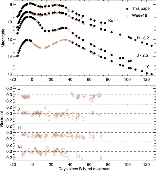
Figure 3. Same as Figure 2 but for the YJHKs bands.
Download figure:
Standard image High-resolution image2.3. NIR Spectroscopy
2.3.1. Data Reduction
Six NIR spectra were taken with FLAMINGOS-2 (Eikenberry et al. 2006) on the Gemini South 8.2 m telescope at the Gemini South Observatory, including the earliest one at only 2.30 days past explosion. The FLAMINGOS-2 spectra were acquired in long-slit mode with the JH grism and filter in place, along with a slit width of 072. This setup yielded wavelength coverage of 1.0–1.8 μm and a resolution of R ∼ 1000. The long-slit spectra were acquired at the parallactic angle with a standard ABBA pattern and reduced in a standard way using the F2 PyRAF package provided by Gemini Observatory. The XTELLCOR pipeline was used to perform telluric corrections and flux calibrations. More details of the data reduction process can be found in Brown et al. (2019) and Hsiao et al. (2019).
Two NIR spectra were provided by the ePESSTO collaboration (Smartt et al. 2015) with the SOFI instrument (Moorwood et al. 1998) on the 3.6 m NTT at La Silla Observatory. The SOFI spectra were observed with blue and red grisms with a slit width of 10, wavelength coverage of 0.9–2.5 μm, and a resolution of R ∼ 500. The conventional ABBA nod-along-the-slit technique was adopted. For each SOFI spectrum, a Vega-like or solar analog was also observed for flux calibration. The SOFI spectra were reduced by performing the following steps: cross-talk correction, flat-field correction, wavelength calibration, sky subtraction, spectral extraction, telluric absorption correction, and flux calibration (Smartt et al. 2015).
Five NIR spectra were observed with FIRE (Simcoe et al. 2013) on the 6.5 m Magellan Baade telescope at Las Campanas Observatory. The FIRE spectra were acquired with the high-throughput prism mode with a slit of 06, wavelength coverage of 0.8–2.5 μm, and a similar resolution as SOFI. For each epoch, the conventional ABBA nod-along-the-slit technique and the sampling-up-the-ramp readout mode were used. Meanwhile, an A0V star was observed for telluric correction close in time, angular distance, and airmass to our science target (Vacca et al. 2003; Hsiao et al. 2015, 2019). The IDL pipeline firehose (Simcoe et al. 2013) was specifically developed to reduce FIRE spectra.
One SpeX (Rayner et al. 2003) spectrum was taken with the 3.0 m NASA IRTF at the summit of Maunakea. The SpeX spectrum was obtained in cross-dispersed mode with a slit of 05, yielding a wavelength range of 0.8–2.5 μm (Hsiao et al. 2019). The data were reduced with the IDL code Spextool (Cushing et al. 2004), which is designed for handling the SpeX data. The flux calibration process for the SpeX spectrograph is similar to that of other devices, such as FIRE, SOFI, and FlAMINGOS-2.
2.3.2. NIR Spectral Diagnostics of SN 2017cbv
Figure 4 shows the NIR spectra obtained for SN 2017cbv, covering the phases from −17.6 to +49.4 days relative to  . The early NIR spectra are dominated by electron scattering with a well-defined photosphere. Thus, the first three early spectra in Figure 4 show relatively featureless blue continua. Later, spectral features develop at 1.05, 1.25, and 1.65 μm when the SN is close to B-band maximum (Wheeler et al. 1998). The most prominent features at those epochs are associated with intermediate-mass species, i.e., O i, Mg ii, and Si iii (see also Figure 2 in Hsiao et al. 2013). Specifically, the strong and relatively isolated absorption feature at 1.05 μm was identified as Mg ii λ1.0927 μm by Wheeler et al. (1998), Hamuy et al. (2002a, 2002b) in SN 1999ee, Gall et al. (2012) in SN 2005ef, and Hsiao et al. (2013) in SN 2011fe. The emission feature at 1.25 μm was identified as Si iii by Hsiao et al. (2013) and Fe iii by Hamuy et al. (2002b) and Rudy et al. (2002). A strong feature around 1.6 μm was identified as Fe iii by Hsiao et al. (2013), Mg ii/Si ii/Co ii by Marion et al. (2009), and Si ii by Wheeler et al. (1998) and Gall et al. (2012). At longer wavelengths, the spectrum is also featureless, except for a weak emission feature around 2.05 μm perhaps due to Si iii (Wheeler et al. 1998).
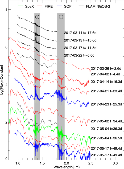
Figure 4. Time-series NIR spectra of SN 2017cbv from NIR spectrographs SpeX, FIRE, SOFI, and FLAMINGOS-2.
Download figure:
Standard image High-resolution imageFigure 5 displays the comparison between SNe 2017cbv and 2011fe at −17.6, −11.5, −2.6, and +4.4 days relative to the B-band maximum (Hsiao et al. 2013). Both spectra are matched very well, except for the Mg ii λ1.0927 μm absorption feature, which is very weak in SN 2017cbv at t = −17.6 and −11.5 days.

Figure 5. Comparison NIR spectra of SN 2017cbv (black) and SN 2011fe (blue) from early epochs through roughly maximum light.
Download figure:
Standard image High-resolution imageTwo weeks past maximum, the spectra showed dramatic evolution dominated by strong emission/absorption features. The Mg ii λ1.0927 μm absorption feature disappeared, and the most remarkable features were the strong and wide peaks around 1.5–1.7 μm, which can be attributed to blends of Co ii, Fe ii, and Ni ii (Wheeler et al. 1998). Meanwhile, new peaks at around 2.2 and 2.4 μm appeared and gradually developed that are mainly attributed to iron-group element Co ii (Wheeler et al. 1998). Figure 6 shows the postmaximum comparisons of SNe 2017cbv, 2011fe (Hsiao et al. 2013), 2012fr (Hsiao et al. 2019), and 2014J (Sand et al. 2016) at comparable phases. They are very consistent with each other at +16.3, +34.4, +36.3, +36.5, and +49.4 days after maximum light. Two spectra were taken at +49.4 days on May 17, one by FIRE and the other by SOFI. We adopted the spectrum observed by FIRE, as the colors from the FIRE spectrum are closer to the NIR-band photometry and the S/N is higher in Figure 4.
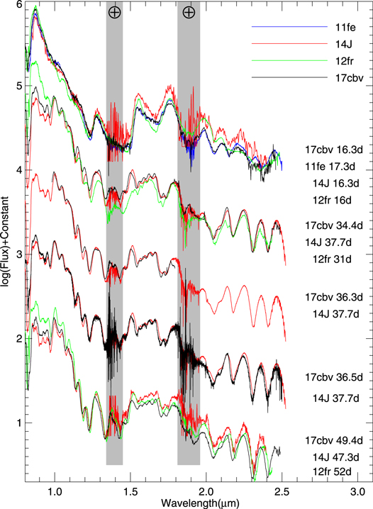
Figure 6. Comparison spectra of SN 2017cbv (black), SN 2011fe (blue), SN 2012fr (green), and SN 2014J (red) after maximum light.
Download figure:
Standard image High-resolution image2.3.3. Mg ii Velocity
A product of explosive carbon burning, Mg ii is a sensitive probe of the location of the inner edge of carbon burning (Wheeler et al. 1998; Marion et al. 2001, 2009; Höflich et al. 2002; Hsiao et al. 2013) in velocity space. The Mg ii λ1.0927 μm line is expected to be observed with decreasing velocity in the early spectral evolution and then to remain at an almost constant velocity when the photosphere has receded below the inner edge of the Mg ii distribution. We can only measure the absorption minimum of the Mg ii λ1.0927 μm line at t = −11.5, −6.6, −2.6, and +4.4 days, with an almost constant velocity of ∼10,500 km s−1. This suggests that its photosphere had receded below the inner edge of magnesium, according to the analysis by Wheeler et al. (1998). Alternatively, Meikle et al. (1996) interpreted the constant velocity of Mg ii as a detached feature.
2.3.4. C i
Unburned carbon provides the most direct diagnostic of the primordial material from the progenitor. The weak-absorption carbon feature was mainly detected from early optical spectra via C ii λ0.6580 μm (Thomas et al. 2007; Scalzo et al. 2010; Silverman et al. 2011; Silverman & Filippenko 2012; Taubenberger et al. 2011; Thomas et al. 2011; Zheng et al. 2013). Alternatively, NIR C i λ1.0693 μm can be taken as a superior carbon tracer compared with the optical C ii λ0.6580 μm, as C i can be detected at maximum light (e.g., Höflich et al. 2002). Hosseinzadeh et al. (2017c) detected a strong C ii λ0.6580 μm feature at t = −19 days, similar to SN 2013dy at t = −16 days (Zheng et al. 2013), although the carbon feature disappeared by day −13 for SN 2017cbv. Very strong carbon C ii was also seen in iPTF 16abc (Miller et al. 2018). We tried to detect the C i from our NIR spectra, and we saw a notch close to λ1.0693 μm near 1.03 μm taken on 2017 April 2, or t ∼ 4.4 days after B-band maximum. We applied the automated spectrum synthesis code SYNAPPS (Thomas et al. 2011) to identify C i λ1.0693 μm, as shown in Figure 7. The blueshift of the C i line (green dashed line in Figure 7) was observed at 11,000 km s−1 at t ∼ 4.4 days after B-band maximum. The velocity of the unburned carbon in the NIR spectrum was consistent with the velocity of Mg ii λ1.0927 μm at the same epoch in Section 2.3.3. If the detected C i is real, SN 2017cbv could be the second case to support the hypothesis that a change in the ionization condition occurs as the temperature cools, indicating that the signature of C ii λ0.6580 μm appears in the very early phase before B-band maximum and C i λ1.0693 μm appears later, i.e., around maximum, as similarly reported by Hsiao et al. (2013) for SN 2011fe. Note that the detection of C i λ1.0693 μm in Figure 7 is interpreted by SYNAPPS (Thomas et al. 2011), which is independent of the very early optical detection of C ii λ0.6580 μm (Hosseinzadeh et al. 2017c).
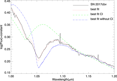
Figure 7. SYNAPPS fit to the region of the C i λ1.069 μm line of SN 2017cbv taken at t ∼ 4.4 days. The spectrum is plotted as a solid black curve, and the best-fit synthesized spectra are plotted with all ions (e.g., C i λ1.069 μm, Mg ii λ1.093 μm, and other ions; red dotted curve), only C i (green dashed curves), and all ions except C i (blue dashed–dotted curves). There is likely a detection of C i in the spectrum, with a clear notch seen in the blue wing of the Mg ii line.
Download figure:
Standard image High-resolution image2.3.5. Paβ
Maeda et al. (2014) emphasized that the Paβ in postmaximum NIR spectra can provide a powerful diagnostic of the presence of unbound hydrogen-rich matter expelled from a companion. Hydrodynamic and radiative transfer models in Maeda et al. (2014) found that the postmaximum Paβ is easily observed, and this feature grows stronger at ∼1–2 months after maximum, covering a range of viewing angles between the observer, SN, and companion star. Sand et al. (2016) tried to identify the Paβ line for the nearby Type Ia SN 2014J. They found no evidence for the presence of Paβ emission after comparing the observed spectra around Paβ λ1.282 μm with the red giant scenario corresponding to 0.3, 0.1, and 0.03 M⊙ of hydrogen for the boundary cases: θ = 0° and 180° (Maeda et al. 2014). Thus, Sand et al. (2016) gave a rough hydrogen mass upper limit of 0.1 M⊙ for all SN–companion star orientations and claimed that it was not distinguishable between the scenario with hydrogen masses of 0.03 M⊙ and observations. We have compared our postmaximum NIR spectra of SN 2017cbv with those of SNe 2011fe, 2012fr, and 2014J at several phases of t = +16.3, +34.4, +36.3, +36.5, and +49.4 days, as shown in Figure 8. We can see that our five postmaximum spectra are well matched with those of SN 2014J, and both have comparable signal-to-noise ratios in Figure 8. No Paβ lines were detected from our five postmaximum NIR spectra by visual inspection, and this yields a similar hydrogen mass limit of less than 0.1 M⊙ from the companion star of SN 2017cbv, although the limit depends on the viewing angles. Analysis of the Paβ line of SN 2017cbv using the same NIR spectrum at 34 days after maximum was performed in Hosseinzadeh et al. (2017c), and they drew similar conclusions. Nondetection of Hα from nebular spectroscopy gave an even lower hydrogen mass limit (Sand et al. 2018).
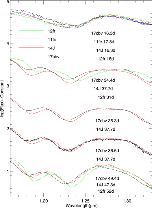
Figure 8. Comparison spectra of Paβ at 1.282 μm for SN 2017cbv in black, SN 2011fe in blue, SN 2012fr in green, and SN 2014J in red after maximum light.
Download figure:
Standard image High-resolution image3. Further Analyses of the Physical Properties of SN 2017cbv
3.1. Light Curves and Color Evolution
3.1.1. Optical Light Curves
Figure 9 shows the BVRIYJHKs-band light curves of SN 2017cbv from our observations (also see Appendix Table 11 for optical and Appendix Table 12 for NIR data). The light curves were sampled during the period t ∼ −16 to +125 days relative to B-band maximum, making SN 2017cbv one of the best-observed SNe Ia in the optical and NIR bands simultaneously. The morphology of the light curves resembles that of normal SNe Ia, showing a shoulder in the R band and a pronounced secondary maximum in the I and NIR bands. The NIR light curves of SN 2017cbv reached their first peak ∼4 days earlier than the B-band curve, consistent with the statistical analysis of an SN Ia sample (Dhawan et al. 2015).
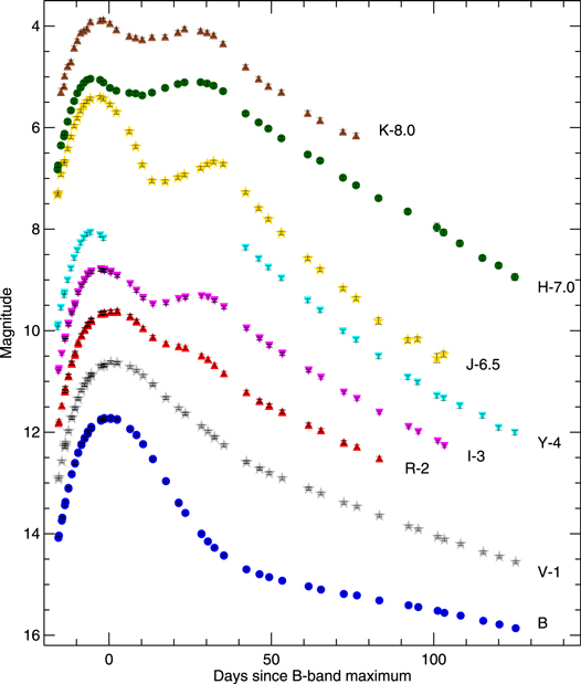
Figure 9. Optical and NIR light curves of SN 2017cbv, spanning about −16 to +125 days with respect to B-band maximum. Data for this figure are available online.(The data used to create this figure are available.)
Download figure:
Standard image High-resolution image3.1.2. Light-curve Parameters
Gaussian process regression (GPR) was applied via the Python module Scikit-learn (Pedregosa et al. 2011) to estimate the light-curve shape parameter Δm15(B) = 0.990 ± 0.013 mag and the peak time of the B-band light curve  MJD, which are used throughout this paper. The value Δm15(B) is the B-band magnitude difference between the peak Bt=0 = 11.710 ± 0.006 mag and 15 days after Bt=15 = 12.700 ± 0.011 mag. The GPR is a nonparametric, Bayesian approach to regression in the area of machine learning (Rasmussen 2006). Similarly, we implemented GPR to fit the phases and maximum peak magnitudes of the VRIYJHKs bands. When possible, we also use the same GPR to deduce the phases and peak magnitudes of the secondary maximum and the minimum magnitude between the two maxima for each of the IYJHKs-band light curves. We follow the nomenclature adopted by Biscardi et al. (2012) to parameterize the light curves of SN 2017cbv. For the X band, at the phases of t1(X), t2(X), and t0(X) relative to B maximum, the first maximum m1(X), the secondary maximum m2(X), and a minimum m0(X) between the two maxima are reached. The uncertainties of the phases were measured using a jackknife procedure. For example, we select N points around the maximum t1 and then start a loop, taking one data point out and fitting with the GPR to the rest of the N − 1 data points. An array of N measurements of t1 is obtained once the loop is completed. Then we do statistics with this array to get the standard deviation σt1, and the final uncertainty of t1 will be
  . We repeat the above process to obtain the uncertainties of t1, t2, and t0 for each band. The light-curve parameters m1, m2, and m0 and their times relative to tBmax (t1, t2, and t0), as well as the decay rate β between 40 and 90 days, are tabulated in Tables 5 and 6. As shown in Elias et al. (1981), the IYJHKs light curves show the first maximum within −2 to −5 days of the B-band maximum, which is consistent with the results for SNe Ia with Δm15 < 1.8 (Folatelli et al. 2010) and in agreement with the statistical studies in the YJH bands (Dhawan et al. 2015). Recent studies suggested that the timing of the i-band maximum indicates the physical state of the SN Ia explosion (González-Gaitán et al. 2014; Ashall et al. 2020). Thus, the time of i-band maximum can be used to subclassify Ia into normal, 91T-like, 03fg-like, 91bg-like, and 02cx-like objects (Figure 3 and Table 1 of Ashall et al. 2020), of which, SN 2017cbv locates in the normal subtype.
Table 5. Light-curve Parameters of SN 2017cbv
| Filter | m(
|
t1a | m1 | t0 | m0 | t2 | m2 | AMilky Way |
|---|---|---|---|---|---|---|---|---|
| (mag) | (days) | (mag) | (days) | (mag) | (days) | (mag) | (mag) | |
| B | 11.710 ± 0.006 | 0.00 ± 0.10 | 11.710 ± 0.006 | ⋯ | ⋯ | ⋯ | ⋯ | 0.615 |
| V | 11.643 ± 0.007 | 1.24 ± 0.10 | 11.637 ± 0.007 | ⋯ | ⋯ | ⋯ | ⋯ | 0.453 |
| R | 11.607 ± 0.008 | 0.66 ± 0.17 | 11.605 ± 0.008 | ⋯ | ⋯ | ⋯ | ⋯ | 0.358 |
| I | 11.840 ± 0.008 | −2.99 ± 0.14 | 11.793 ± 0.007 | 15.32 ± 0.22 | 12.472 ± 0.012 | 26.98 ± 0.11 | 12.312 ± 0.012 | 0.256 |
| Y | ⋯ | −4.74 ± 0.09 | 12.050 ± 0.020 | ⋯ | ⋯ | ⋯ | ⋯ | 0.175 |
| J | 12.004 ± 0.018 | −3.57 ± 0.19 | 11.883 ± 0.015 | 16.74 ± 0.77 | 13.613 ± 0.024 | 31.66 ± 0.69 | 13.206 ± 0.018 | 0.122 |
| H | 12.180 ± 0.018 | −4.72 ± 0.13 | 12.027 ± 0.016 | 7.79 ± 0.20 | 12.343 ± 0.016 | 25.96 ± 0.29 | 12.085 ± 0.016 | 0.078 |
| Ks | 11.938 ± 0.017 | −3.07 ± 0.27 | 11.877 ± 0.015 | 12.77 ± 0.35 | 12.252 ± 0.017 | 25.33 ± 0.44 | 12.064 ± 0.016 | 0.052 |
Note.
aThe t1, t2, and t0 are phases of the first maximum m1, the secondary maximum m2, and the minimum m0 between the two maxima relative to B maximum.Download table as: ASCIITypeset image
Dhawan et al. (2015) also studied the YJH-band light curves of 91 SNe Ia from the literature and made an extensive statistical analysis for NIR light-curve shape parameters, i.e., t1, t0, and t2, and late-time decay β in these three bands. We found that the phases t1, t0, and t2 for SN 2017cbv in Table 5 for each band are consistent with values reported by Dhawan et al. (2015). As predicted by Kasen (2006), a larger Ni mass of SN leads to higher temperatures and thus a later  recombination wave occurring around 7000 K, which tends to delay the secondary maximum. The epoch of secondary maximum t2 was slightly delayed for SN 2017cbv, perhaps indicating a larger Ni mass, when compared with SN 2011fe, which shows an earlier secondary maximum. The SN 2011fe has Δm15 = 1.18 mag (Zhang et al. 2016), which also indicated a lower Ni mass.
After the (secondary) maximum, the light curves of SNe Ia usually show a linear decline in magnitude. We also calculated the decay rate β for SN 2017cbv in the BVRIYJHKs bands during the phases 40 days < t < 90 days. The values of the decay rate in different bands are listed in Table 6. Our optical decline rates β are consistent with those reviewed by Leibundgut (2000). In the early nebular phase, the NIR-band light curves of SN 2017cbv are found to have faster decay rates than the optical ones, consistent with the results reported by Dhawan et al. (2015). As noted by Dhawan et al. (2015), SNe Ia tend to have similar late-time decay rates in the NIR bands. At late time, the SN gradually becomes transparent to the γ rays produced by radioactive decays. Similar late-time decay rates perhaps suggest a similar internal structure of the explosions, which is also in agreement with the predictions for Chandrasekhar-mass models (Woosley et al. 2007) that produce different nickel masses but with similar radial distributions of iron-group elements.
3.1.3. Milky Way Extinction
The Milky Way extinction in the BVRIJHKs bands toward SN 2017cbv was derived from the dust maps of Schlafly & Finkbeiner (2011) in individual bandpasses, CTIO B, V, R, and I and 2MASS J, H, and Ks, which are similar to the ANDICam filters used in the paper. The extinction values are listed in the last column of Table 5.30 The Galactic reddening toward SN 2017cbv is E(B − V) = 0.162 mag (Schlafly & Finkbeiner 2011).
The Y-band extinction AY = 0.175 was estimated by considering the mean RV-dependent extinction law, and we refer to Equations (1), (2a), and (2b) in Cardelli et al. (1989),


where x is the reciprocal of the Y-band central wavelength at λ = 1.03 μm (Hillenbrand et al. 2002), the ratio of total to selective extinction is RV = 3.1, and the V-band extinction toward SN 2017cbv is AV = 0.453 (Schlafly & Finkbeiner 2011).
The Na i D lines in the high-resolution spectrum provide an independent measurement of both the Milky Way and host reddening. Burns et al. (2020) published one high-resolution spectrum of SN 2017cbv using the Magellan Inamori Kyocera Echelle (MIKE; Bernstein et al. 2003) in their Figure 5. The Na i D lines can be seen toward the Milky Way, but no Na i D lines are seen toward the host galaxy. A higher Milky Way reddening of E(B − V) = 0.23 ± 0.16 mag was obtained based on the equivalent width (EW) of the Na i D lines (Burns et al. 2020). This may further suggest that SN 2017cbv suffers some Milky Way reddening but negligible host reddening. Ferretti et al. (2017) also published five high-resolution spectra of SN 2017cbv with the Ultraviolet and Visual Echelle Spectrograph (UVES; Dekker et al. 2000) and found low values of EW for the Na i (D1 and D2) lines, consistent with negligible host reddening.
3.1.4. Comparison to Other SNe Ia
Figure 10 shows comparisons of the optical light curves of SN 2017cbv with those of well-observed normal SNe Ia, i.e., SN 2001el (Δm15 = 1.15 mag; Krisciunas et al. 2003), SN 2002dj (Δm15 = 1.08 mag; Pignata et al. 2008), SN 2003du (Δm15 =1.02 mag; Stanishev et al. 2007), SN 2004S (Δm15 = 1.10 mag; Krisciunas et al. 2007), SN 2005cf (Δm15 = 1.07 mag; Wang et al. 2009b), SN 2011fe (Δm15 = 1.18 mag; Zhang et al. 2016), SN 2012cg (Δm15 = 0.86 mag; Marion et al. 2016), SN 2012fr (Δm15 = 0.82 mag; Zhang et al. 2014; Contreras et al. 2018), and SN 2014J (Δm15 = 1.08 mag; Foley et al. 2014; Marion et al. 2015; Srivastav et al. 2016; Li et al. 2019a). The comparison sample includes all available normal SNe Ia that have been well observed in the optical/NIR bands and have similar light-curve shapes as SN 2017cbv. It can be seen that the near-maximum-light curves of SN 2017cbv are very similar to the comparison sample. The late-time decay rate during the interval t = 40–90 days after the peak denoted as β here was estimated for the BVRIYJHKs bands,31 and the corresponding values are listed in Table 6. The BVRI-band late-time decay rates β of SN 2017cbv appear relatively slower than or similar to those of the corresponding rates of the comparison sample. More details can be seen in Table 6 and Figure 10. During 20–90 days after B maximum, the B magnitude of SN 2017cbv falls in between that of SN 2012fr and SN 2011fe; this suggests that these SNe Ia have different 56Co hard-gamma-ray escaping ratios from the ejecta.
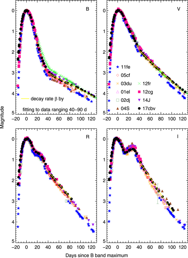
Figure 10. Comparison of BVRI-band light curves of SN 2017cbv with other well-observed SNe Ia: SNe 2001el (Krisciunas et al. 2003), 2002dj (Pignata et al. 2008), 2003du (Stanishev et al. 2007), 2004S (Krisciunas et al. 2007), 2005cf (Wang et al. 2009b), 2011fe (Pereira et al. 2013; Zhang et al. 2016), 2012cg (Marion et al. 2016), 2012fr (Zhang et al. 2014; Contreras et al. 2018), and 2014J (Foley et al. 2014; Marion et al. 2015; Srivastav et al. 2016; Li et al. 2019a). The yellow solid lines mark the decay rate β during the interval t = 40–90 days after B maximum.
Download figure:
Standard image High-resolution imageTable 6. The Decay Rate β of the Comparison Sample in the BVRI Bands
| Name | βBa | βV | βR | βI |
|---|---|---|---|---|
| (mag(100 days)−1) | (mag(100 days)−1) | (mag(100 days)−1) | (mag(100 days)−1) | |
| SN 2017cbv | 1.442 ± 0.057 | 2.555 ± 0.033 | 3.139 ± 0.037 | 4.029 ± 0.049 |
| SN 2005cf | 1.663 ± 0.050 | 2.639 ± 0.036 | 3.215 ± 0.035 | 4.381 ± 0.061 |
| SN 2011fe | 1.397 ± 0.004 | 2.762 ± 0.005 | 3.249 ± 0.023 | 4.236 ± 0.047 |
| SN 2012fr | 1.639 ± 0.015 | 2.683 ± 0.031 | ⋯ | ⋯ |
| SN 2014J | 1.334 ± 0.024 | 2.852 ± 0.042 | 3.355 ± 0.064 | 4.248 ± 0.099 |
| SN 2001el | 1.493 ± 0.097 | 2.638 ± 0.072 | 3.221 ± 0.094 | 4.244 ± 0.059 |
| SN 2004S | 1.608 ± 0.114 | 2.704 ± 0.107 | 3.185 ± 0.094 | 3.773 ± 0.064 |
| SN 2003du | 1.707 ± 0.033 | 2.626 ± 0.043 | 3.094 ± 0.066 | 4.577 ± 0.127 |
| βYa | βJ | βH |

|
|
| SN 2017cbv | 5.288 ± 0.053 | 6.033 ± 0.121 | 4.092 ± 0.046 | 4.034 ± 0.173 |
| SN 2012fr | 5.345 ± 0.041 | 6.167 ± 0.110 | 4.133 ± 0.039 | ⋯ |
Note.
aThe late-time decay rate β of the light curve during the interval t = 40–90 days relative to .
.
Download table as: ASCIITypeset image
In Figure 11, the YJHKs-band light curves of SN 2017cbv are compared with those of SNe 2001el, 2002dj, 2003du, 2004S, 2005cf, 2011fe, 2012cg, 2012fr, and 2014J. The overall light curves of SN 2017cbv in the YJHKs bands resemble the comparison SNe in Figure 11 and Table 6. One can see that their secondary maximum features show some differences, and these variations might be related to the progenitor metallicity, the concentration of iron-group elements, and the abundance stratification in SNe Ia (Kasen 2006). After t > 90 days, the light-curve decay slope in the NIR bands becomes less steep; this could be influenced by the Co ii, like mid-IR Co ii λ10.5 μm time-series variation, flattening out at about day 90–100 (Telesco et al. 2015).
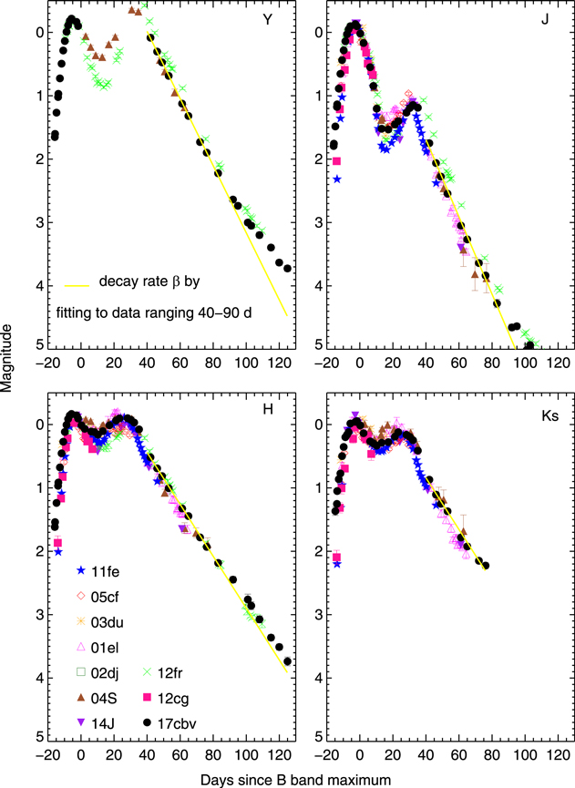
Figure 11. Same as Figure 10 but for YJHKs-band light curves. The late-time decay rates β of SN 2017cbv are also overplotted with the yellow solid lines.
Download figure:
Standard image High-resolution image3.1.5. Color Curves
A comparison of several well-observed SNe is shown in Figures 12–14. All photometry has been corrected for reddening in the Galaxy and the host galaxies by the values from the corresponding published papers, except for SN 2017cbv, for which only the Galactic extinction was corrected. The optical color curves of SN 2017cbv and the comparison sample (B − V, V − R, and V − I) are presented in Figure 12. At very early phases, t < −10 days with respect to B-band maximum, the colors of SN 2017cbv are much bluer than the comparison SNe (also see Hosseinzadeh et al. 2017c; Stritzinger et al. 2018; Bulla et al. 2020). The B − V color of SN 2017cbv stays flat at about −0.05 mag soon after explosion and then slowly becomes bluer until day −5. Also, it is the bluest SN in colors B − V, V − R, and V − I until day −11. The V − R color is even bluest among all comparison SNe Ia until 10 days after B maximum. The blue colors seen in the early light curves of some SNe Ia have been interpreted as interactions between SN ejecta and a companion star, serving as evidence in favor of the SD scenario (Brown et al. 2012; Marion et al. 2016; Hosseinzadeh et al. 2017c; Dimitriadis et al. 2019a). After B-maximum light, the color evolution of SN 2017cbv matches well with the comparison sample and the Lira–Phillips relation (blue solid line; Phillips et al. 1999) at about 30 days past maximum. For a nearby SN Ia sample in the Lira law regime, Förster et al. (2013) claimed that the B − V slope −0.013 mag day−1 can be used to classify the faster and slower decliners. Faster decliners (<−0.013 mag day−1) have a higher EW of Na i D lines, redder colors, and a lower RV reddening law at maximum light, suggesting the presence of circumstellar material (Wang et al. 2009a, 2013, 2019; Förster et al. 2013), while slower decliners are the opposite. The slope of SN 2017cbv in the Lira phase is −0.010 mag day−1; thus, it is a slower decliner. This is consistent with the very small EW measurements of Na i absorption lines for SN 2017cbv (Ferretti et al. 2017) and blue B − V color at maximum light.

Figure 12. The B − V, V − R, and V − I color curves of SN 2017cbv, together with those of SNe 2001el, 2002dj, 2003du, 2004S, 2005cf, 2011fe, 2012cg, 2012fr, and 2014J. All of the comparison sample has been dereddened. Only the Milky Way extinction for SN 2017cbv was corrected. The blue solid line in the B − V panel displays the unreddened Lira–Phillips loci. The data sources are cited in the text; see Section 3.1. The inset panel is a zoom-in of the very early phase color curves. The corresponding shape parameter Δm15 of each SN is listed in parentheses behind the SN name.
Download figure:
Standard image High-resolution image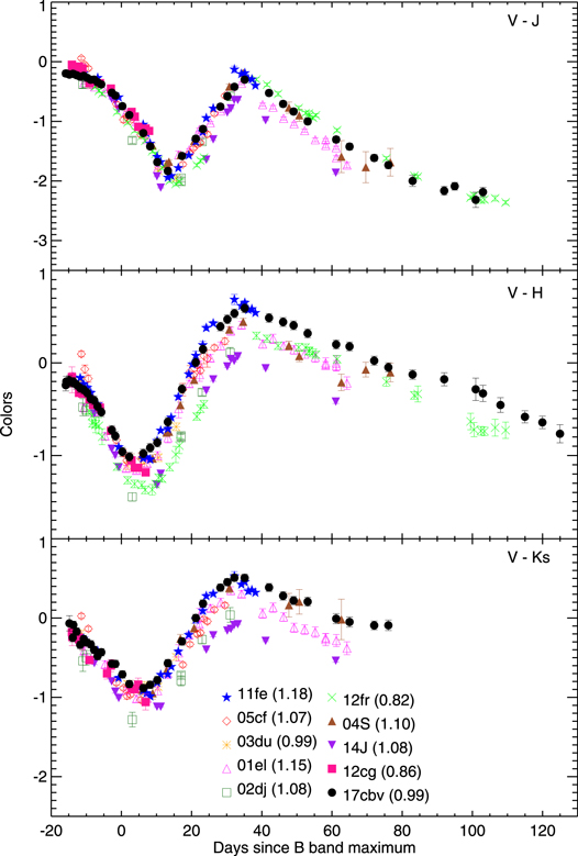
Figure 13. The V − JHKs color curves of SN 2017cbv compared with SNe 2001el, 2002dj, 2003du, 2004S, 2005cf, 2012cg, 2011fe, 2012cg, 2012fr, and 2014J. The corresponding shape parameter Δm15 of each SN is listed in parentheses behind the SN name.
Download figure:
Standard image High-resolution image
Figure 14. The J − H and H − Ks color curves of SN 2017cbv, together with the comparison sample SNe 2001el, 2002dj, 2003du, 2004S, 2005cf, 2011fe, 2012cg, 2012fr, and 2014J. The phases t1, t0, and t2 in the J band are overplotted with dashed lines in the top panel. The corresponding shape parameter Δm15 of each SN is listed in parentheses behind the SN name.
Download figure:
Standard image High-resolution imageWe also compare the V − NIR color evolution (V − J, V − H, and V − Ks) of SN 2017cbv and the comparison SNe Ia in Figure 13. We can see that the V − NIR color evolution of SN 2017cbv matches with the comparison sample, especially the well-observed SN 2011fe. The study by Burns et al. (2014) derived empirical relations of intrinsic colors V − J and V − H at maximum light relative to the light-curve shape parameter sBV in their Table 2. According to the relations for their low-reddening sample (LRS), and assuming an sBV = 1.11 for SN 2017cbv (Burns et al. 2020), we obtained intrinsic colors (V − J)hostmax = −0.61 ± 0.08 and  mag. Meanwhile, Table 5 gives the observed colors
  and
and  mag at maximum epochs. Thus, we can derive
  and
and  mag. This indicates that SN 2017cbv suffers neglected host reddening.
The J − H and H − Ks color evolutions of SN 2017cbv and the comparison SNe Ia are shown in Figure 14. Overplotted are the phases of the first maximum t1 = −3.6 days, the secondary maximum t2 = 31.7 days, and the minimum between the two maxima t0 = 16.7 days in the J band relative to B-band maximum, as shown by the vertical dashed lines. As seen from the top panel of Figure 14, the J − H color illustrates a pronounced evolution after t1. The flux in the J band decreases obviously with respect to the H band shortly after t1, probably due to the lack of emission features around 1.2 μm (Spyromilio et al. 1994; Hoflich et al. 1995; Wheeler et al. 1998). This trend holds until t2, when the Fe ii λ1.25 μm emission line forms. Then, the J − H color becomes redder again as a result of a faster decline rate in the J band. The bottom panel of Figure 14 displays the H − Ks plot, and SN 2017cbv matches well with the comparison SNe.
3.2. CMD
The SNe Ia are assumed to be standard distance candles after a one- or two-parameter (light-curve shape/color) correction. If they form a one- or two-parameter group, it is possible to derive distance measurements from their multicolor light curves. Wang et al. (2003) studied the color–magnitude relation of SNe Ia during the first month past maximum and found a linear relation between B and B − V color in SNe Ia. This linear relation provides distance determinations and dust extinction estimates simultaneously. The color–magnitude intercept calibration (CMAGIC) method provides a tool to obtain accurate distance calibration without data around optical maximum and suggests new observational strategies to estimate accurate distances (Wang et al. 2003; Conley et al. 2006; Wang et al. 2006; He et al. 2018).
The CMDs of SN 2017cbv are shown in Figure 15, together with those of SN 2011fe. For the first, second, and fourth rows, the first column shows the diagram for the observed magnitudes, the second column shows the diagram after correction for Milky Way extinction, and the third column shows the CMD after reddening corrections based on various assumptions. Note that on the CMD, the two SNe show genuine differences, as indicated by the differences in their CMD shapes. With the high-quality NIR data on both SNe, we can use the CMDs to estimate the extinction to these SNe. However, some assumptions need to be made to allow this. In the original CMAGIC construction, Wang et al. (2003) used the linear region of the CMD, but there are more features that can be employed by the extensive data on these SNe. Examples are the bluest and reddest colors on the CMD. The CMDs of B versus B − Ks and V versus V − Ks show a characteristic upside down "&"-shaped curve. Various aspects of this shape can be used to analyze the properties of the SNe.
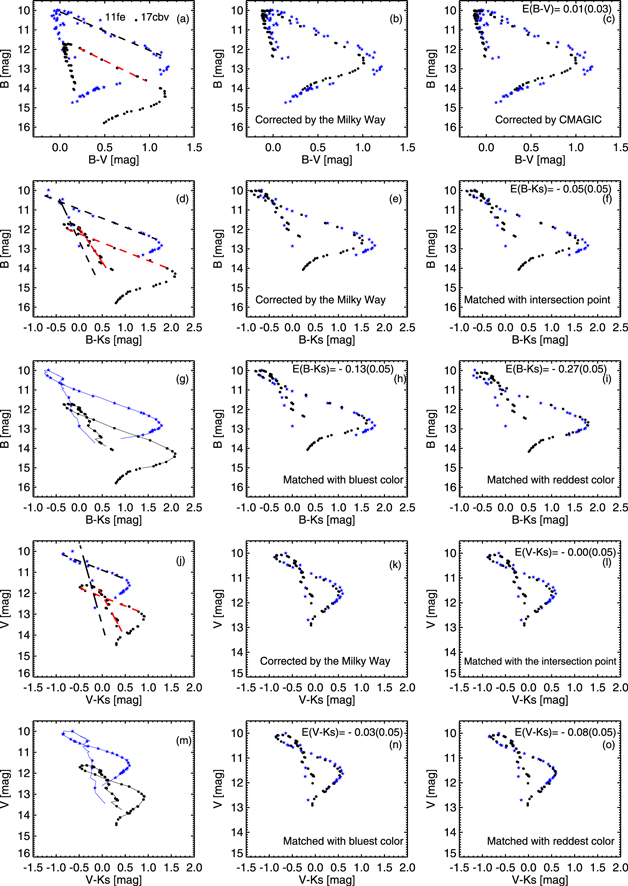
Figure 15. Color–magnitude plots of SNe 2017cbv and 2011fe for B − V, B − Ks, and V − Ks colors, from top to bottom. Overplots are (CMAGIC) linear fitting (dashed lines) and the interpolation to the BVKs bands of SNe 2017cbv and 2011fe (solid lines). Refer to the text for details.
Download figure:
Standard image High-resolution image3.2.1. B − V Color
Figure 15(a) shows the CMD presented by Wang et al. (2003, 2006). In order to estimate the CMAGIC color excess EBV(B − V), we use the quantity as defined in Wang et al. (2003),

where Bmax is the B-band maximum, and βBV and BBV denote the slope and the value for the intercept at (B − V) = 0 for the linear region from 5 to 27 days after the B-band maximum with the CMAGIC relation (Wang et al. 2003):

The CMAGIC color excess for a reddening-free SN  0 also depends on the light-curve shape parameter Δm15(B), and the linear relationship between them was derived from a low-extinction sample of SNe Ia (Phillips et al. 1999; Wang et al. 2003):
The final color excesses of SNe Ia can be measured based on the equation

We fit the B magnitude and B − V color of SNe 2017cbv and 2011fe between 5 and 27 days, and we derived EBV(B − V)11fe = 0.030 ± 0.044 and EBV(B − V)17cbv = 0.173 ± 0.029 mag, which includes both the contribution from the Milky Way and the SN's host galaxy. We can take SN 2011fe as a reference with no dust extinction from the Milky Way and its host galaxy (Nugent et al. 2011; Johansson et al. 2013; Patat et al. 2013). The SN 2017cbv has negligible host extinction, E(B − V)host = 0.011 ± 0.029 mag, after considering the Milky Way extinction toward SN 2017cbv (Schlafly & Finkbeiner 2011).
The distance of the two SNe can also be derived based on the CMAGIC method by comparing the observed BBV and the absolute value  from the empirical relation between the absolute magnitude
  versus Δm15 in Figure 10 of Wang et al. (2003). Table 3 of Wang et al. (2003) gives the fit result to the absolute magnitude
  versus
  relation for RB = 3.3, expressed as
The extinction correction ABV is given by Equation 3(a) of Wang et al. (2003), expressed as

where RB = 3.3, βBV = 2.250 ± 0.030, and E(B − V)17cbv(host) = 0.011 ± 0.029 mag. The observable value BBV is the color–magnitude intercept, which is calculated from the intercept of the typical color B − V = 0.6 mag reported by Wang et al. (2003). To minimize the covariance of the distance estimates to the slope βBV, Wang et al. (2003) defined the following equation to measure BBV as the standard color–magnitude intercept:

Equation (14) yields BBV = 11.648 ± 0.030 mag for SN 2017cbv. Thus, we obtained the distance modulus μ = 30.58 ± 0.05 mag (D = 13.1 ± 0.3 Mpc) after applying  , ABV, and BBV in Equation (17) in Section 3.4.1. Based on the same method, we estimated the distance modulus μ = 29.14 ± 0.10 mag for SN 2011fe, which is consistent with the Cepheid distance modulus of SN 2011fe (Shappee & Stanek 2011).
3.2.2. B − Ks Color
Wang et al. (2003) also found that B magnitudes and the various colors (i.e., B − R, B − I) are linearly related. Thanks to our well-observed optical and NIR photometric observations, we found that the B magnitude versus B − Ks color and V magnitude versus V − Ks color are also linearly related in the phase ranges of 5 days ≤ t ≤ 30 days and t ≤ −5 days. The two linear relations have an intersection point for SN 2017cbv (red dashed lines) and SN 2011fe (black dashed lines), as shown in panels (d) and (j) of Figure 15. If we assume that SN 2017cbv and SN 2011fe are intrinsically the same, matching their corresponding colors should give us the comparable interstellar dust extinctions. There are no first-principle physical insights to help us determine which points on the CMDs are most representative of the intrinsic color of the SN Ia population. To explore the various possibilities, we tested the color excesses E(B − Ks) and E(V − Ks) by matching the reddest color, bluest color, and intersection point between SN 2017cbv and SN 2011fe.
We plot the B versus B − Ks diagram in panels (d)–(i) of Figure 15. Panels (d)–(f) are the observations without extinction corrections of the Milky Way and the host, only corrections of the Milky Way, and corrections of the Milky Way and its host by matching with the intersection point of two dashed lines (black for SN 2011fe and red for SN 2017cbv). One line is the linear fit to the phase interval 5 days ≤ t ≤ 30 days relative to B-band maximum, and the other is the linear fit to the phase range t ≤ −5 days. Thus, we obtained E(B − Ks)host = −0.05 ± 0.05 mag in panel (f).
Figure 15(g) is the same as Figure 15(d), except that the solid lines are the interpolation values to B and Ks in the phase range of −15 days ≤ t ≤ 60 days after B-band maximum. When matching the bluest color of SN 2017cbv with that of SN 2011fe in panel (h), we obtained E(B − Ks)host = −0.13 ± 0.05 mag. While matching the reddest color of SN 2017cbv with that of SN 2011fe in panel (i), we obtained E(B − Ks)host = −0.27 ± 0.05 mag.
Based on these four different assumptions on the uniformity of the intrinsic color, we obtained four different values of E(B − Ks). Among them, matching the reddest color yields the most negative values of E(B − Ks) = −0.27 ± 0.05 mag. This value is inconsistent with the CMAGIC estimates. It would imply a significant overcorrection of the Milky Way reddening if the reddest color is used as the reference point for extinction correction. It is more likely that the difference at the reddest color is intrinsic to the SNe, and, contrary to what has been employed in the Lira–Phillips relation, the late-time color cannot be used as reliable estimates of extinction, at least for these two very well observed SNe.
3.2.3. V − Ks Color
Similar to the previous section, we also plot V versus V − Ks in panels (j)–(o) of Figure 15. By matching with the intersection point of the two lines for SNe 2017cbv and 2011fe, we obtained E(V − Ks)host = −0.00 ± 0.05 mag in panel (l). By matching with the bluest and reddest colors, we obtained E(V − Ks)host = −0.03 ± 0.05 mag in panel (n) and E(V − Ks)host = −0.08 ± 0.05 mag in panel (o), respectively.
We note further that the intrinsic colors B − Ks and V − Ks of SN 2017cbv are bluer than the expected value of SN 2011fe when matching them with the intersection point, the bluest color, and the reddest color: panels (f) and (l), (h) and (n), and (i) and (o) in Figure 15, respectively. We assumed no host extinction for SN 2011fe based on the reddening analysis and distance determination on our CMAGIC diagram (in Section 3.2.1) and other work by Nugent et al. (2011), Johansson et al. (2013), and Patat et al. (2013).
We also note that the B − V color of SN 2017cbv in panel (c) is bluer than that of SN 2011fe by 0.18 ± 0.07 mag around t ∼ 32 days; at this phase, the two SNe have the reddest color. This suggests that SN 2017cbv and SN 2011fe are different in the B and/or V bands at some late phases. When we matched the reddest colors B − Ks of SN 2017cbv with SN 2011fe, the estimated color excess E(B − Ks) of the host in panel (i) is different from the early-phase estimates (matching with the bluest color or intersection point) by 2σ–3σ in panels (f) and (h). In contrast, the color excess E(V − Ks) of the two SNe by matching their reddest color in panel (o) is comparable with the measurements by matching the bluest color in panel (n) and intersection point in panel (l). This may further suggest that the B magnitudes between SN 2017cbv and SN 2011fe are more different than the V magnitudes at these late phases, although the B and V magnitudes of SN 2017cbv are brighter than those of SN 2011fe after B-band maximum in Figure 10, where their maxima are matched.
3.3. More on Host Reddening E(B − V)
In addition to the insights derived from the CMD, there are several other mature methods for deriving the host galaxy reddening.
3.3.1. Phillips Intrinsic Color
Phillips et al. (1999) compiled a set of unobscured SNe Ia and derived a relation between their intrinsic pseudocolor (Bmax − Vmax)0 and their decay parameter Δm15(B):
This relation allows one to estimate the host reddening suffered by any normal SN Ia by just comparing their measured pseudocolor and intrinsic estimate. After correcting by Milky Way reddening, SN 2017cbv shows a pseudocolor (Bmax − Vmax) that is even bluer than the expected value from Phillips et al.'s (1999) relation, or E(B − V)host = −0.006 ± 0.016 mag. This value corresponds to an E(B − Ks) of about −0.019 mag, which is inconsistent with the value estimated by matching the late-time CMD in B versus B − Ks, suggesting again that the late-time colors of SNe Ia can be substantially different.
3.3.2. Lira–Phillips Relation
The top panel of Figure 12 shows the B − V color evolution curve, and the unreddened Lira–Phillips loci is overplotted with a blue solid line. The following relation was derived to describe the intrinsic B − V color evolution in the phase interval 30 days ≤ tV ≤ 90 days (Lira 1996; Phillips et al. 1999):

Applying the relation to SN 2017cbv, we obtain a host extinction of E(B − V)host = 0.000 ± 0.037 mag.
3.3.3. CMAGIC Diagram
Wang et al. (2003) derived the CMAGIC relation for SNe Ia over the phase interval 5 days ≤ tB ≤ 27 days after B-band maximum. We applied the CMAGIC relation to SN 2017cbv in Section 3.2, and we derived the host extinction E(B − V)host = 0.011 ± 0.029 mag.
By averaging the host extinction of SN 2017cbv based on the above three methods, we obtained E(B − V)host = 0.002 ± 0.009 mag. The low host galaxy reddening is consistent with the fact that the SN exploded at the outskirts of NGC 5643 and no narrow Na i D absorption lines were detected in the low-resolution spectra, even in the MIKE spectrum (Burns et al. 2020). Ferretti et al. (2017) published five high-resolution spectra of SN 2017cbv and found values of EW for Na i (D1 and D2) at the lower end of the empirical relation between strength of Na i D absorption versus reddening (Poznanski et al. 2012), consistent with zero reddening. Thus, we assume no host galaxy reddening for SN 2017cbv in our study.
3.4. Distance of SN 2017cbv
3.4.1. NIR Absolute Calibration
The effects of extinction are considerably reduced in the JHKs bands, and it seems there are relatively constant peak magnitudes in the NIR bands (Meikle 2000; Krisciunas et al. 2004a, 2004b, 2007). The SNe Ia have a more uniform peak luminosity in the NIR bands (Krisciunas et al. 2004a; Wood-Vasey et al. 2008; Folatelli et al. 2010; Matheson et al. 2012; Phillips 2012; Avelino et al. 2019). The well-sampled NIR photometry of SN 2017cbv can be used to determine the distance modulus toward NGC 5643. For each band, the apparent maximum magnitudes m1 and the magnitudes at  are listed in the third column of Table 7 and the fourth and second columns, respectively, of Table 5. For each case, we used the following formula to derive the distance modulus μ:
- 1.Here m stands for the apparent magnitudes, M represents the absolute NIR magnitudes from these calibration sources (Krisciunas et al. 2004a; Mandel et al. 2009; Wood-Vasey et al. 2008; Folatelli et al. 2010; Burns et al. 2011; Kattner et al. 2012), and all assume a Hubble constant H0 = 72 km s−1 Mpc−1 (Freedman et al. 2001; Spergel et al. 2007).
- 2.The Milky Way extinction AMilky Way toward SN 2017cbv was adopted with AJ = 0.122, AH = 0.078, and
 = 0.052 mag (Schlafly & Finkbeiner 2011).
 - 3.The host extinction AHost of SN 2017cbv was assumed to be zero based on the analysis presented in Section 3.3.
- 4.The SCorrection was applied between our JHKs-band magnitudes on the 2MASS system and the CSP-calibrated magnitude (Contreras et al. 2010) for the calibration sources (Folatelli et al. 2010; Burns et al. 2011; Kattner et al. 2012). They are SCorrection(J) = 0.005, SCorrection(H) = −0.038, and SCorrection(Ks) = 0.009 mag, which are added to the CSP-calibrated magnitudes. The remaining calibration sources have been calibrated to the 2MASS system (Persson et al. 1998), and no SCorrection is necessary.
- 5.No KCorrection has been applied to our photometry due to the close distance of SN 2017cbv.

Table 7. Derived Distance Moduli μ of NGC 5643
| Calibration Source | Filter | Apparent Magnitudea | Absolute Magnitude | Distance Modulus μ |
|---|---|---|---|---|
| to NGC 5643 (mag)b | ||||
| Mandel et al. (2009)c | J | 12.004 ± 0.018 | −18.25 ± 0.17 | 30.13 ± 0.17 |
| H | 12.180 ± 0.018 | −18.01 ± 0.11 | 30.11 ± 0.11 | |
| Ks | 11.938 ± 0.017 | −18.25 ± 0.19 | 30.14 ± 0.19 | |
| Wood-Vasey et al. (2008)c,d | J | 12.004 ± 0.018 | −18.29 ± 0.33 | 30.17 ± 0.33 |
| H | 12.180 ± 0.018 | −18.08 ± 0.15 | 30.18 ± 0.15 | |
| Ks | 11.938 ± 0.017 | −18.32 ± 0.26 | 30.21 ± 0.26 | |
| Folatelli et al. (2010)c | J | 12.004 ± 0.018 | −18.42 ± 0.18 | 30.30 ± 0.18 |
| H | 12.180 ± 0.018 | −18.23 ± 0.19 | 30.37 ± 0.19 | |
| Ks | 11.938 ± 0.017 | −18.30 ± 0.27 | 30.18 ± 0.27 | |
| Krisciunas et al. (2004a)e | J | 11.883 ± 0.015 | −18.57 ± 0.14 | 30.33 ± 0.14 |
| H | 12.027 ± 0.016 | −18.24 ± 0.18 | 30.19 ± 0.18 | |
| Ks | 11.877 ± 0.015 | −18.42 ± 0.12 | 30.24 ± 0.12 | |
| Folatelli et al. (2010)e | J | 11.883 ± 0.015 | −18.43 ± 0.18 | 30.19 ± 0.18 |
| H | 12.027 ± 0.016 | −18.42 ± 0.19 | 30.41 ± 0.19 | |
| Ks | 11.877 ± 0.015 | −18.47 ± 0.27 | 30.29 ± 0.27 | |
| Burns et al. (2011)e | J | 11.883 ± 0.015 | −18.44 ± 0.12 | 30.20 ± 0.12 |
| H | 12.027 ± 0.016 | −18.26 ± 0.10 | 30.25 ± 0.10 | |
| Kattner et al. (2012)e,f | J | 11.883 ± 0.015 | −18.57 ± 0.14 | 30.33 ± 0.14 |
| H | 12.027 ± 0.016 | −18.42 ± 0.14 | 30.41 ± 0.14 | |
Notes.
aThe apparent magnitude in Table 7 is the same as that from Table 5. bThe distance modulus μ was derived by combining absolute calibration sources with the apparent magnitudes (see text for details). Only Milky Way extinctions toward to SN 2017cbv were corrected with AJ = 0.122, AH = 0.078, AKs = 0.052 mag (Schlafly & Finkbeiner 2011). We assumed H0 = 72 km s−1 Mpc−1 (Freedman et al. 2001; Spergel et al. 2007). cFiducial time corresponds to B-band maximum brightness. dUsing the PAIRITEL subsample only. eFiducial time corresponds to the first maximum brightness in the given filter (J, H, or Ks). fUsing subsample 2 of Kattner et al. (2012).Download table as: ASCIITypeset image
According to Equation (17), the distance modulus to SN 2017cbv ranges from 30.11 ± 0.11 mag (D = 10.5 ± 0.5 Mpc) to 30.41 ± 0.19 mag (D = 12.1 ± 1.1 Mpc), shown in Figure 16 and listed in Table 7. Note that the uncertainty of each case in Table 7 is dominated by the calibration of the absolute NIR peak magnitude. We note that the same absolute calibrations were applied to the JHKs magnitudes of SN 2011fe by Matheson et al. (2012), yielding a dispersion of 0.31 mag, very similar to the case of SN 2017cbv.

Figure 16. Distance moduli toward NGC 5643 from our work on SN 2017cbv with NIR absolute calibration, a SNooPy fit to the BVRIYJHKs light curves, and a CMAGIC diagram. Other estimates toward NGC 5643 are also listed here for comparison. Sand et al. (2018) estimated the distance modulus of SN 2017cbv, μ = 30.45 ± 0.09 mag, via an MLCS2k2 fit (Jha et al. 2007) to the light curve obtained by Las Cumbres Observatory's 1 m telescope. The CSP II group measured the distance modulus of SN 2013aa, μ = 30.55 ± 0.08 mag, via a light-curve template fitter (Burns et al. 2020). Bottinelli et al. (1985) listed the redshift-independent distance modulus of NGC 5643, μ = 31.14 ± 0.40 mag, from the Tully–Fisher method. Error bars are 1σ.
Download figure:
Standard image High-resolution image3.4.2. SNooPy Fitting
SNooPy is a well-established light-curve fitting method to generate template light curves in the CSP natural system and derive distances to SNe Ia (Burns et al. 2011). Applying SNooPy to our BVRIYJHKs-band light curve, we obtained a distance modulus of μ = 30.46 ± 0.08 mag (Burns et al. 2014), or distance D = 12.4 ± 0.5 Mpc. This distance estimate should be an independent measurement of CSP (Burns et al. 2020), as we have independent data. When we calibrated the optical using the CSP calibration (Burns et al. 2020), we established some correlation there.
3.4.3. CMAGIC Diagram
Comparing the measurement of the color–magnitude intercept parameter BBV to its absolute value in Table 3 of Wang et al. (2003), we obtained μ = 30.58 ± 0.05 mag for SN 2017cbv (D = 13.1 ± 0.3 Mpc).
The CMDs (B versus B − V, B versus B − Ks, and V versus V − Ks in Section 3.2) in Figure 15 give Δμ17cbv(B) = 1.10 mag relative to SN 2011fe. Assuming a Cepheid distance μ11fe = 29.04 ± 0.19 mag for SN 2011fe (Shappee & Stanek 2011), we obtained a distance modulus μ17cbv = 30.14 ± 0.19 mag for SN 2017cbv (D = 10.7 ± 0.9 Mpc).
3.4.4. Distance of SN 2013aa
Burns et al. (2020) applied three methods to the photometric data of SN 2013aa to estimate its distance modulus. They are μ = 30.46 ± 0.08 mag from SNooPy fitting (Burns et al. 2011, 2014), μ = 30.56 ± 0.04 mag from the MLCS2k2 fitter (Jha et al. 2007), and μ = 30.62 ± 0.04 mag from the SALT2 algorithm (Guy et al. 2007), respectively (assuming H0 = 72 km s−1 Mpc−1). The adopted three methods yield an average estimate of SN 2013aa μ = 30.55 ± 0.08 mag. The SN 2013aa also exploded in the same galaxy with SN 2017cbv, which provides an independent distance determination of SN 2017cbv. The SN 2013aa was discovered by the Backyard Observatory Supernova Survey (BOSS) on 2013 February 13 (Parker et al. 2013) and classified as an SN Ia (Parrent et al. 2013). The SN 2013aa is 74'' west and 180'' south of the core of the host galaxy NGC 5643 (Graham et al. 2017).
In summary, we measured the distance of SN 2017cbv with three methods: NIR absolute calibration, SNooPy fitting, and the CMAGIC diagram. These derived values in Figure 16 are consistent with the results (μ = 30.45 ± 0.09 mag, D = 12.3 ± 0.5 Mpc; Sand et al. 2018) made via the MLCS2K2 fitter (Jha et al. 2007) using independent data and the value μ = 31.14 ± 0.40 mag (D = 16.9 ± 3.1 Mpc) determined from the Tully–Fisher method (Bottinelli et al. 1985; Tully & Fisher 1988). Individually, the distance moduli of SN 2017cbv from NIR absolute calibration (μ = 30.11 ± 0.11 to 30.41 ± 0.19 mag) are smaller than the light-curve template fitters with SNooPy for our data and MLCS2k2 for independent data (Sand et al. 2018), consistent within 2.6σ. The NIR absolute calibration values are also smaller than the CMAGIC diagram, consistent within 2.5σ, except for the smallest value (μ = 30.11 ± 0.11 mag) in the H band, calibrated with Mandel et al. (2009).
Another SN Ia, SN 2013aa, exploded in NGC 5643 and provided an independent distance to NGC 5643 (Burns et al. 2020), consistent with our measurements. Going forward, we adopt our CMAGIC results for the distance to this galaxy (μ = 30.58 ± 0.05 mag) to estimate the quasi-bolometric luminosity, and we compare with theoretical models in the following section.
3.5. Bolometric Light Curve
The SN 2017cbv was also observed with the Ultra-Violet Optical Telescope (UVOT; Roming et al. 2005) on board the Swift satellite (Gehrels et al. 2004), spanning t = −18.5 to ∼14 days relative to the B-band maximum light (Hosseinzadeh et al. 2017c). The UV photometric observations were performed in the UVW2, UVM2, and UVW1 filters. Hosseinzadeh et al. (2017c) published the reduced data, and the photometry was performed using the pipeline for the Swift Optical Ultraviolet Supernova Archive (SOUSA; Brown et al. 2014).
We construct the spectral energy distribution (SED) evolution of SN 2017cbv using the published UVM2 photometry (Hosseinzadeh et al. 2017c) and our optical/NIR-band data, covering wavelengths of 1800–25000 Å. We ignored the UVW2 and UVW1 photometry due to their known red leaks (Brown et al. 2010). The SED method in SNooPy (Burns et al. 2011, 2014) was used to estimate the uvoir quasi-bolometric light curve of SN 2017cbv. The real photometry of each band was matched with the synthetic photometry on the spectral template from Hsiao et al. (2007), and then the matched spectral template for each phase was integrated from 1800 to 25000 Å, which we took as the quasi-bolometric luminosity. The light-curve fitting model "max_model" in SNooPy was used to interpolate the missing data points (Prieto et al. 2006). For the infrared flux at wavelengths longward of  , the Rayleigh–Jeans law is assumed. No host reddening is assumed due to our former analysis in Section 3.3, and the CMAGIC distance modulus of SN 2017cbv was applied to calculate the bolometric luminosity.
Table 8 tabulates the quasi-bolometric light curve of SN 2017cbv using SNooPy (Burns et al. 2011). The bolometric light curve can be used to estimate the nickel mass synthesized during the explosion using Arnett's rule (Arnett 1982). This rule associates the bolometric rise time and the maximum bolometric luminosity Lmax with the energy deposition ENi contributed by the radioactive decay chain 56Ni  Co
Co  Fe within the expanding ejecta (Stritzinger & Leibundgut 2005). The association can be simply expressed as Lmax = αENi, where α is the ratio of input to released energy with a value around 1 (Branch 1992; Hoeflich & Khokhlov 1996; Stritzinger & Leibundgut 2005; Scalzo et al. 2014a).
Table 8. The Estimated Quasi-bolometric Luminosity of SN 2017cbv by Adopting the CMAGIC Distance Modulus of SN 2017cbv; μ = 30.58 mag and Ho = 72 km s−1 Mpc−1
| Phasea | Lbolb | Phase | Lbol |
|---|---|---|---|
| −15.56 | 0.198 | 17.34 | 0.550 |
| −14.56 | 0.278 | 21.26 | 0.459 |
| −13.57 | 0.355 | 23.30 | 0.429 |
| −12.55 | 0.466 | 28.24 | 0.373 |
| −11.55 | 0.593 | 30.23 | 0.352 |
| −10.55 | 0.717 | 32.22 | 0.326 |
| −9.55 | 0.872 | 35.13 | 0.289 |
| −8.56 | 0.994 | 42.03 | 0.208 |
| −7.60 | 1.101 | 46.04 | 0.179 |
| −6.61 | 1.212 | 49.02 | 0.162 |
| −5.55 | 1.301 | 53.01 | 0.149 |
| −4.15 | 1.386 | 61.10 | 0.119 |
| −2.56 | 1.447 | 64.90 | 0.108 |
| −1.58 | 1.462 | 71.90 | 0.089 |
| 0.42 | 1.438 | 75.92 | 0.083 |
| 2.40 | 1.384 | 82.80 | 0.070 |
| 6.37 | 1.158 | 91.76 | 0.059 |
| 7.74 | 1.055 | 94.75 | 0.056 |
| 8.32 | 1.038 | 100.70 | 0.050 |
| 9.66 | 0.930 | 102.76 | 0.047 |
| 10.33 | 0.894 | 107.73 | 0.042 |
| 11.58 | 0.812 | 114.67 | 0.036 |
| 13.11 | 0.726 | 119.63 | 0.033 |
| 13.33 | 0.716 | 124.62 | 0.031 |
Notes.
aDays since B-band maximum. bThe unit is 1043 erg s−1.Download table as: ASCIITypeset image
Figure 17 shows the uvoir quasi-bolometric light curve of SN 2017cbv. Overplotted are the bolometric light curves of the normal SNe Ia 2011fe (Zhang et al. 2016), 2005cf (Wang et al. 2009b), and 2012fr (Contreras et al. 2018) for comparison, which are the few other SNe Ia to have been well observed in the UV, optical, and NIR. The GPR fitting was again applied to determine the bolometric rise time and peak luminosity, shown in the top panel of Figure 17. The peak luminosity of SN 2017cbv is Lpeak = 1.48 × 1043 erg s−1, or log (Lpeak/erg s−1) =43.17 dex, which is consistent with the DDT scenario in the Chandrasekhar-mass models with the peak bolometric luminosity log (Lpeak/erg s−1) = 42.80–43.31 dex (Hoeflich & Khokhlov 1996; Seitenzahl et al. 2013b; Kromer et al. 2016; Hoeflich et al. 2017). The peak luminosity of SN 2017cbv is also consistent with other models, i.e., sub-Chandrasekhar-mass double detonation models (Fink et al. 2010; Kromer et al. 2010), pulsational DDT models (Hoeflich & Khokhlov 1996; Dessart et al. 2014), and so on.
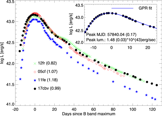
Figure 17. The UV through NIR quasi-bolometric light curve of SN 2017cbv with the CMAGIC distance modulus μ = 30.58 mag of SN 2017cbv. Overplotted are quasi-bolometric light curves of well-observed normal SNe 2005cf (Wang et al. 2009b), 2011fe (Zhang et al. 2016), and 2012fr (Contreras et al. 2018) for comparison. The inset panel shows the GPR fit to the peak of the bolometric light curve of SN 2017cbv.
Download figure:
Standard image High-resolution image3.6. Nickel Mass
3.6.1. Nickel Mass from uvoir Bolometric Light Curve
In calculation of the bolometric luminosity, we adopt the CMAGIC distance modulus of SN 2017cbv, μ = 30.58 ± 0.05 mag, which is close to the external independent distance determination of SN 2013aa (Burns et al. 2020) exploded in the same galaxy. This gives a peak luminosity Lpeak = 1.48 ± 0.07 × 1043 erg s−1 and a synthesized nickel mass MNi = 0.73 ± 0.03 M⊙, which is used throughout this paper.
3.6.2. Nickel Mass from the Phase of the Secondary Maximum in the YJH Bands
Kasen (2006) attributed the secondary maximum of NIR emission to the ionization evolution of iron-group elements in the ejecta and predicted that the secondary maximum should be delayed for larger Fe masses, indicating that the phase of the secondary maximum should be a function of the nickel mass in the explosion. This was investigated by recent studies (Biscardi et al. 2012; Jack et al. 2012; Dhawan et al. 2015, 2016). Dhawan et al. (2016) studied the correlation between the phase of the secondary maximum t2 and the bolometric peak luminosity and established the Lpeak versus t2 relations for the YJH-band light curves. The well-sampled optical and NIR observations of SN 2017cbv presented in this paper offer a good chance to test the above-derived nickel mass using the reddening-free and distance-independent method. The time t2 was measured to be 31.66 ± 0.69 and 25.96 ± 0.29 days from the J- and H-band photometry, and the corresponding peak bolometric luminosities are 1.25 ± 0.17 and 1.11 ± 0.27 × 1043 erg s−1, yielding 0.62 ± 0.08 and 0.55 ± 0.13 M⊙ nickel masses, respectively. The corresponding value derived from the Y-band data is 0.66 ± 0.10 M⊙ if we adopt its corresponding secondary maximum of 33.83 ± 0.45 days according to Wee et al. (2018).
We measured the nickel mass of SN 2017cbv using two methodologies that employ the quasi-bolometric light curve and the phases of the secondary maximum in the NIR bands. Those derived values of the nickel mass are listed in Tables 9 and 10, which are consistent with each other within 2σ, and comparable to those of normal SNe Ia such as SN 2005cf (MNi = 0.78 M⊙; Wang et al. 2009b), SN 2011fe (MNi ∼ 0.57 M⊙; Zhang et al. 2016), SN 2012cg (MNi ∼ 0.72 M⊙; Chakradhari et al. 2019), and SN 2012fr (MNi ∼ 0.60 M⊙; Contreras et al. 2018). Our measured nickel mass is matched with some Mch DDT models and sub-Mch double detonation models discussed in Section 4, while the BV-band light curves of SN 2017cbv are matched with Mch DDT model 25 with a nickel mass of 0.6 M⊙ after B maximum.
Table 9. 56Ni Mass Estimated from uvoir Bolometric Light Curves
| Method | μa | Lpeak | Ni Massa |
|---|---|---|---|
| (mag) | (1043 erg s−1) | (M⊙) | |
| CMAGIC Distance of SN 2017cbv | 30.58 ± 0.05 | 1.48 ± 0.07 | 0.73 ± 0.03 |
Note.
aUsing alpha parameter of 1.0.Download table as: ASCIITypeset image
Table 10. 56Ni Mass Related to the Time of the Second Maximum for YJH Bands
| Methoda | Band | t2 | Lpeak | Ni Massb |
|---|---|---|---|---|
| (days) | (1043 erg s−1) | (M⊙) | ||
| Lmax = (0.041 ± 0.005) × t2 + (−0.065 ± 0.122) | Y | 33.83 ± 0.45 | 1.32 ± 0.21 | 0.66 ± 0.10 |
| Lmax = (0.039 ± 0.004) × t2 + (0.013 ± 0.106) | J | 31.66 ± 0.69 | 1.25 ± 0.17 | 0.62 ± 0.08 |
| Lmax = (0.032 ± 0.008) × t2 + (0.282 ± 0.174) | H | 25.96 ± 0.29 | 1.11 ± 0.27 | 0.55 ± 0.13 |
Notes.
aThe correlation coefficient values between Lmax and t2 were taken from Table 2 in Dhawan et al. (2016). bUsing alpha parameter of 1.0.Download table as: ASCIITypeset image
3.7. Is SN 2017cbv a Normal Type Ia?
Figure 18 shows the bolometric luminosity (1800–25000 Å) and the separate contributions of the NIR (9000–25000 Å), optical (3000–9000 Å), and UV (1800–3000 Å) portions of the spectrum for SNe 2005cf, 2011fe, 2012fr, and 2017cbv. All results were derived using the SNooPy module (Burns et al. 2011, 2014). The UVM2, Johnson–Cousins UBVRI, and 2MASS JHKs filters were applied to the multiband data of SNe 2005cf (Wang et al. 2009b) and 2011fe (Zhang et al. 2016). The UVM2 and CSP natual filters uBgVriYJH were applied to the multiband light curves of SN 2012fr (Contreras et al. 2018). The UVM2, ANDICam BVRI, Y, and 2MASS JHKs filters were applied to our data of SN 2017cbv. The CSP natural filter function Y was used for SN 2017cbv, as no ANDICam filter function for the Y band is available. There are no obvious differences for the bolometric (∼0.1%) and NIR (∼1%) luminosities if we ignore the Y filter. We adopted the following host extinctions and distance moduli: E(B − V)host = 0.1 mag and μ = 32.31 mag for SN 2005cf (Wang et al. 2009b), E(B − V)host = 0 mag and μ = 29.04 mag for SN 2011fe (Zhang et al. 2016), E(B − V)host = 0.03 mag and μ = 31.27 mag for SN 2012fr (Contreras et al. 2018), and E(B − V)host = 0 mag and μ = 30.58 mag for SN 2017cbv. All of the Milky Way extinctions toward the four SNe are corrected according to Schlafly & Finkbeiner (2011). The missing photometry for each epoch was interpolated by the light-curve fitting model "max_model" (Prieto et al. 2006) in SNooPy. For the infrared flux at wavelengths longward of the reddest wavelength, a Rayleigh–Jeans law is assumed. An SED-based method is used to estimate the bolometric luminosity by integrating the spectral template for each phase from Hsiao et al. (2007) × a factor, so the synthetic photometry of the template matches the real photometry.
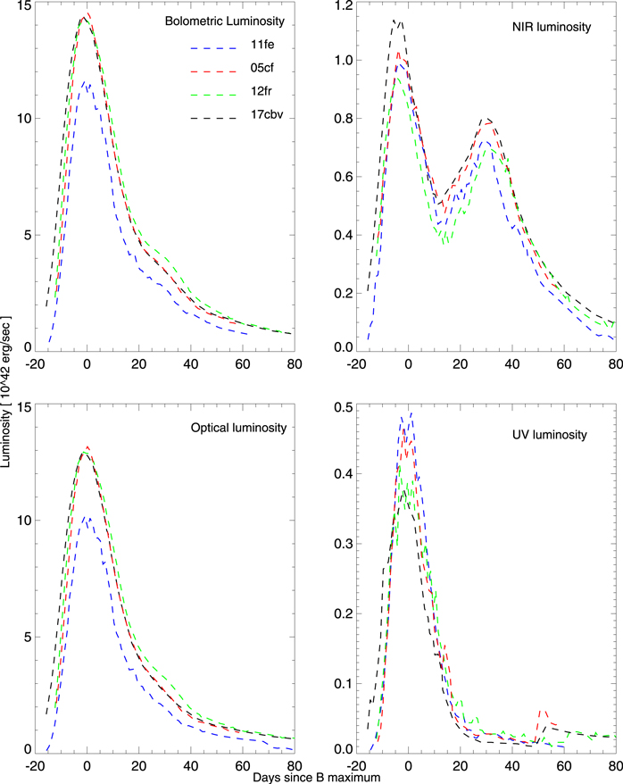
Figure 18. Bolometric (1800–25000 Å), NIR (9000–25000 Å), optical (300–9000 Å), and UVM2 (1800–3000 Å) luminosity of SNe 2005cf, 2011fe, 2012fr, and 2017cbv derived with the same SNooPy method (Burns et al. 2011).
Download figure:
Standard image High-resolution imageAs shown in Figure 18, SNe 2005cf, 2012fr, and 2017cbv have comparable bolometric luminosity, and all of them are brighter than SN 2011fe. The bolometric light curves of these four SNe are matched with their optical contribution, showing that optical luminosity of an SN Ia dominates the bolometric luminosity. The NIR and UV contributions to the bolometric light curves are generally of less importance than the optical. We note that these four SNe Ia have comparable NIR and UV luminosities.
Figure 19 illustrates the UV and NIR contributions to the bolometric light curves in the top panel and the optical contribution in the bottom panel. Overplotted are the flux ratios of SN 2011fe (Zhang et al. 2016) and SN 2012fr (Contreras et al. 2018). The flux ratios measured by SNooPy, Zhang et al. (2016), and Contreras et al. (2018) point to differences among these SNe (i.e., the different NIR fraction of SN 2011fe shown in bottom panel of Figure 19); however, when the flux ratios are measured with the same methodology as we use here, the flux ratios seem completely consistent. Contreras et al. (2018) applied two methods (photometric trapezoidal integration and spectral template fitting) to calculate the luminosity of SN 2012fr based on UVM2 and uBgVriYJH-band magnitudes. The first method calculates the flux from the observed photometry by trapezoidal integration of the fluxes derived from each filter. The UV contribution is made from Swift UVM2 photometry, and the NIR contribution at wavelength λ > λH is estimated from the Rayleigh–Jeans law. The second method is similar to the SED method in SNooPy. More detailed steps can be found in Appendix B of Contreras et al. (2018). The bolometric luminosities from the two methods are consistent at the ±5% level (e.g., Figure 29 of Contreras et al. 2018). Our flux fraction estimated by the SED method in the SNooPy module is consistent with that of the two methods and much more consistent with the spectral template fitting method (e.g., the UV fraction in the top panel of Figure 19).
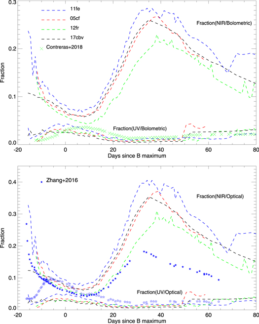
Figure 19. Top: ratio of the NIR (9000–25000 Å) and UV (1800–3000 Å) fluxes to all (1800–25000 Å) fluxes for SNe 2005cf, 2011fe, 2012fr, and 2017cbv with the same method (dashed lines). The UV fraction of SN 2012fr is overplotted from Contreras et al. (2018). Bottom: ratio of the NIR (9000–25000 Å) and UV (1800–3000 Å) fluxes to the optical (3000–9000 Å). The UV and NIR fractions of SN 2011fe are overplotted from Zhang et al. (2016). Zhang et al. (2016) formed SED curves with UVW2 and UVW1, which are ignored in our analysis due to their red leaks (Brown et al. 2010). The difference of the NIR fraction of SN 2011fe is caused by difference methods. Refer to the text for details.
Download figure:
Standard image High-resolution imageZhang et al. (2016) adopted the photometric direct integration method based on Swift UVW2, UVM2, UVW1, and UBVRIJHKs-band photometry, which computes the effective wavelength of each filter and converts the measured magnitude to flux to generate an SED, thus integrating the derived SED at specific wavelength ranges for bolometric (1600–24000 Å), UV (1600–3200 Å), optical (3200–9000 Å), and NIR (9000–24000 Å) luminosities. Our UV fraction of SN 2011fe is smaller than that of Zhang et al. (2016), as we did not use the fluxes of filters UVW2 and UVW1 due to their red leaks (Brown et al. 2010). Our NIR fraction is larger than that of Zhang et al. (2016), mainly because we use different methods to calculate them and Zhang et al. (2016) did not assume a Rayleigh–Jeans law for the infrared flux at wavelength λ >  .
.
Figures 18 and 19 illustrate that SN 2017cbv shows similar behaviors as the normal, well-observed SNe Ia SN 2005cf, SN 2011fe, and SN 2012fr. These normal characteristics can also be seen in their light curves (e.g., Figures 10 and 11) and color curves (e.g., Figures 12–14). This behavior is further seen in the NIR spectra from early to late phases relative to B-band maximum (e.g., Figures 5 and 6). All of our multiband photometry and NIR spectra point to SN 2017cbv as a normal SN Ia. However, the very early colors (B − V, V − R, and V − I) of SN 2017cbv are bluer than the normal comparison sample in Figure 12. Also, the early flux of SN 2017cbv is brighter than both SNe 2005cf and 2012fr with a similar bolometric peak, although the difference gradually disappears when close to maximum phase. For example, at the very early phase of SN 2012fr (t = −11.3 days), the flux ratios of SN 2017cbv over SN 2012fr are 1.7, 1.4, 1.7, and 2.9 for the bolometric flux, NIR, optical, and UV contributions, respectively.
The SN 2017cbv shares similar early characteristics (i.e., early light-curve excess and/or blue color) with SN 2012cg (Marion et al. 2016), iPTF16abc (Miller et al. 2018), MUSSES 1604D (Jiang et al. 2017; Maeda et al. 2018), SN 2018oh (Dimitriadis et al. 2019a; Li et al. 2019b; Shappee et al. 2019), and SN 2019yvq (Miller et al. 2020). The early light-curve excess could be the result of either ejecta interaction with its companion (Kasen 2010; Marion et al. 2016; Hosseinzadeh et al. 2017c) or vigorous mixing of radioactive 56Ni in the SN outermost ejecta (Dessart et al. 2014; Piro & Morozova 2016; Magee et al. 2018, 2020; Miller et al. 2018; Magee & Maguire 2020). It could also be associated with the He-detonation configuration within a WD with an He layer (Jiang et al. 2017; Maeda et al. 2018; Polin et al. 2019; Tanikawa et al. 2019). From the observational perspective, early-color observations of SNe Ia suggest a "red" class showing a steep transition from red to bluer colors and a "blue" class with bluer colors and flatter evolution (Stritzinger et al. 2018). Based on a sample of 13 SNe Ia discovered within 3 days from inferred first light, Stritzinger et al. (2018) claimed that events in the blue class are overluminous and of the branch shallow silicon spectral type, while ones in the red class are more typically related to the branch core-normal, or CooL, type (Branch et al. 2006). Jiang et al. (2018) inspected the light curves of 23 young SNe Ia and drew similar conclusions. Also, Han et al. (2020) confirmed the above claim of the distinction between blue and red by adding six events to the sample of Stritzinger et al. (2018). From a theoretical perspective, models are expected to have red colors early on when 56Ni is produced in the high-density innermost regions of ejecta and later show a transition to blue colors with the photosphere receding into increasing hotter layers. In contrast, the following scenarios predict blue colors soon after explosion involving the interaction of SN ejecta with a nondegenerate companion star (Kasen 2010), unbound material ejected prior to detonation (pulsational DDT models; Dessart et al. 2014), radioactive 56Ni mixing in the SN outer ejecta (Piro & Morozova 2016; Miller et al. 2018; Magee et al. 2018, 2020; Magee & Maguire 2020; Bulla et al. 2020), or an ejecta–disk-originated matter (DOM) collision in the DD scenario (Levanon & Soker 2017, 2019).
4. Theoretical Perspectives
From a theoretical perspective, several kinds of explosion models can be expected to generate SNe Ia. Here we examine two popular explosion models: the Mch DDT scenario and the sub-Mch double detonation scenario. Both scenarios have received much attention, as they reproduce aspects of SN Ia light curves and spectra (Höflich 1995; Hoeflich & Khokhlov 1996; Kasen et al. 2009; Kromer et al. 2010; Röpke et al. 2012; Sim et al. 2013; Blondin et al. 2015; Maeda et al. 2018; Polin et al. 2019). Thus, both scenarios could make an important contribution to the SN Ia population (Hachisu et al. 2008; Mennekens et al. 2010; Ruiter et al. 2011; Scalzo et al. 2014b; Goldstein & Kasen 2018). In detail, Seitenzahl et al. (2013a) showed that ∼50% of SNe Ia should explode at or near Chandrasekhar in order to interpret the solar abundance of manganese observed in the Galaxy. Scalzo et al. (2014b) showed the empirical fits to the light curves of the SDSS and SNLS SNe Ia, which suggests 30% of these events originating from the sub-Chandrasekhar scenario.
4.1. Mch DDT Scenario
In the Mch DDT scenario (Khokhlov 1991; Höflich 1995; Plewa et al. 2004; Röpke & Niemeyer 2007; Kasen et al. 2009; Blondin et al. 2013; Seitenzahl et al. 2013b; Hoeflich et al. 2017), a WD is thought to accrete material from a nondegenerate companion star and explode following carbon ignition near the WD center, which occurs when the WD mass has nearly reached Mch. The DDT models involve a transition from deflagration to detonation burning, which is parameterized by a transition density ρtr, regulating the preexpansion of the WD and determining the abundance structure during the deflagration phase (Hoeflich et al. 2017). The DDT scenario predicts some of the basic characteristics of SNe Ia, i.e., the spherical geometry of SN Ia remnants with layered chemical structures (Rest et al. 2008; Hoeflich et al. 2017), spherical density distributions as suggested by small continuum polarization (Patat et al. 2012), and so on.
As mentioned in Section 3.5, the peak luminosity of SN 2017cbv is located in the parameter space of the Chandrasekhar-mass DDT models. Here we compared the BV-band light curves of SN 2017cbv with three typical DDT models in Hoeflich et al. (2017) in Figure 20. Models 23 (Höflich et al. 2002), 23d5 (Höflich et al. 2006; Diamond et al. 2015), and 25 (Höflich et al. 2002) are assumed to have solar metallicity and a main-sequence mass of 5 M⊙, with different central (ρc = 2.0, 6.0, and 2.0 × 10⁹ g cm−3) and transition (ρtr = 2.3, 2.3, and 2.5 × 10⁷ g cm−3) densities at the time of the explosion. The corresponding 56Ni masses for DDT models 23, 23d5, and 25 are 0.56, 0.54, and 0.60 M⊙. At phases t ≥ 0 since the B-band maximum, model 25 is more consistent with the BV-band data. Compared with model 23, model 25 has a larger transition density ρtr, meaning less deflagration burning and subsequently higher density burning during the detonation phase (Hoeflich et al. 2017). Model 25 has log (Lpeak/erg s−1) = 43.22 dex and provides an absolute brightness MV = −19.29 mag with a rise time of 18.5 days. Model 25 is fainter than the observed peak for SN 2017cbv by 0.15 mag but well within the error bars of the distance and reddening uncertainties.

Figure 20. Absolute BVRI-band light curves of SN 2017cbv. The CMAGIC distance modulus μ = 30.58 ± 0.05 mag, and no host extinctions were applied to our BVRI-band data. The Milky Way extinctions toward SN 2017cbv are corrected following Schlafly & Finkbeiner (2011). Overplotted are the Mch DDT and sub-Mch double detonation models of normal-bright SNe Ia for comparison. Typical DDT models 23, 23d5, and 25 in Hoeflich et al. (2017) are overplotted and assume a progenitor of solar metallicity and 5 M⊙ on the main sequence, with different central (ρc = 2.0, 6.0, and 2.0 × 10⁹ g cm−3) and transition (ρtr = 2.3, 2.3, and 2.5 × 10⁷ g cm−3) densities at the time of the explosion, respectively. Sub-Mch model 4 is composed of a C/O core mass Mcore = 1.125 M⊙ and a shell mass Msh = 0.039 M⊙, and model 3 is composed of a C/O core mass Mcore = 1.025 M⊙ and a shell mass Msh = 0.055 M⊙ (Kromer et al. 2010; Fink et al. 2010), while sub-Mch model 3c is a bare C/O core with Mcore = 1.025 M⊙ (Kromer et al. 2010).
Download figure:
Standard image High-resolution image4.2. Sub-Mch Double Detonation Scenario
In the sub-Mch double detonation model (Nomoto 1980; Taam 1980; Livne 1990; Shen & Bildsten 2009; Fink et al. 2010; Kromer et al. 2010; Woosley & Kasen 2011; Moll & Woosley 2013; Blondin et al. 2017; Wang et al. 2017; Shen et al. 2018a), the explosion is triggered by the detonation of a helium shell that may be accreted from a helium companion star. This helium detonation then triggers a second detonation in the core. Observational signatures of sub-Mch WD explosions point to two categories of helium shell sizes. Thick shell models predict an early-time flux excess caused by the presence of radioactive material in the ashes of the helium shell, but this flux excess will be red due to line blanketing. Thin helium shell models can reproduce the characteristics of many normal SNe Ia and subluminous SN 1991bg–like objects (Shen et al. 2018b; Polin et al. 2019).
Here we choose double detonation and bare CO detonation in sub-Chandrasekhar-mass WDs. For the double detonation scenarios, we take models 3 and 4 of Fink et al. (2010) and Kromer et al. (2010) as thick shell models. Model 3 yields 0.55 M⊙ of 56Ni from an initial WD with a 1.025 M⊙ CO core and an He shell of 0.055 M⊙. In the initial helium shell detonation, 1.7 × 10⁻³ M⊙ of 56Ni, 6.2 × 10⁻³ M⊙ of 52Fe, and 4.4 × 10⁻³ M⊙ of 48Cr have been synthesized close to the ejecta surface. Model 4 yields 0.78 M⊙ of 56Ni from an initial WD with a 1.125 M⊙ CO core and an He shell of 0.039 M⊙. In the initial helium shell detonation, 4.4 × 10⁻³ M⊙ of 56Ni, 3.5 × 10⁻³ M⊙ of 52Fe, and 2.2 × 10⁻³ M⊙ of 48Cr have been synthesized close to the ejecta surface. As a bare CO detonation, we use model 3c of a detonation of 1.025 M⊙ that yields 0.55 M⊙ of 56Ni (Kromer et al. 2010), which represents the extreme case of a thin helium shell model.
Models 3, 3c, and 4 are available for the optical spectral time series from the Heidelberg Supernova Model Archive.32 The synthetic photometry for these models in the ANDICam BVRI bands is shown in Figure 20. We obtained MB,max = −19.4, MV,max = −19.9, MR,max = −19.3, and MI,max = −19.5 mag for model 4 and MB,max = −18.6, MV,max = −19.5, MR,max = −19.3, and MI,max = −19.3 mag for model 3. For model 3c, the values are MB,max = −19.2, MV,max = −19.4, MR,max = −18.9, and MI,max = −19.0 mag. Those calculated peak values are similar to the ones given by Kromer et al. (2010) for the model parameters in their Table 1. As shown in Figure 20, the V band of model 4 is higher than the observations of SN 2017cbv after t ∼ −5 days relative to B-band maximum. In contrast, models 3c and 3 predict comparable V peaks but fainter B peaks, especially for model 3 with the faintest B-band curve. As the DDT models do, sub-Chandrasekhar models 3, 3c, and 4 predict narrower light-curve profiles (rising and declining) than the observations. The shoulder-phase R band of models 3 and 4 is higher than the observations, while model 3c is comparable with the observations at the same phase. For the I band, models 3, 3c, and 4 are brighter than the observations of SN 2017cbv at shoulder phase.
The observations of SN 2017cbv are not compatible with sub-Chandrasekhar models due to their brighter V-band peak magnitudes for model 4 and much fainter B-band magnitudes for model 3, or the redder B-V colors of models 3, and 4 (Table 1 of Kromer et al. 2010). We note that the sub-Chandrasekhar bare core detonation model 3c does not predict such red colors as models 3 and 4, but it expects a fainter magnitude at maximum phase in the RI bands and brighter magnitudes at the shoulder phase in the I band.
As shown in Figure 20, Chandrasekhar DDT model 25 is more matched with the observations of SN 2017cbv compared with other DDT models, sub-Chandrasekhar double detonation models 3 and 4, and bare core detonation model 3c. However, for the early phase, model 25 still does not match with the observations of SN 2017cbv due to its broader rising light curve. As discussed in Hosseinzadeh et al. (2017c) for the same SN, extra energy is likely to make a considerable contribution to the early-phase light curve. The early light-curve excess could be the result of either ejecta interaction with its companion (Kasen 2010; Marion et al. 2016; Hosseinzadeh et al. 2017c) or vigorous mixing of radioactive 56Ni in the SN outermost ejecta (Dessart et al. 2014; Piro & Morozova 2016; Magee et al. 2018, 2020; Miller et al. 2018; Magee & Maguire 2020). More detailed discussion of the early phase of SN 2017cbv will be presented by Sand et al. (in preparation). Our well-observed data provide a valuable reference to model the detailed explosion of SN 2017cbv from very early to late phases.
5. Conclusions
The optical and NIR-band photometric observations acquired for SN 2017cbv constitute the most complete temporal coverage in eight bands simultaneously among the current SN Ia sample, even for the well-observed SN 2011fe and SN 2012fr. We also present more than 10 time-series NIR spectra, with the first observed only 2.3 days past explosion (−17.6 days after maximum), the earliest normal SN Ia target, similar to early-phase NIR spectra only observed for SN 2011fe (Hsiao et al. 2013). These make it an ideal reference for comparative investigations of SNe Ia. Here are our main conclusions.
- 1.The SN 2017cbv is a typical normal SN Ia with a decline rate parameter Δm15(B) = 0.990 ± 0.013 mag and peak B-band magnitude mag when taking the distance modulus of SN 2017cbv as μ = 30.58 ± 0.05 mag utilizing the CMAGIC diagram.
- 2.The NIR spectra of SN 2017cbv are also well matched with normal SNe Ia, i.e., SN 2011fe, SN 2012fr, and SN 2014J, from the very early phase to about 50 days after B-band maximum.
- 3.The C i λ1.0693 μm near 1.03 μm was likely identified from our NIR spectrum taken at t ∼ 4.4 days via SYNAPPS (Thomas et al. 2011), with a clear notch seen in the blue wing of the Mg ii line. Its blueshifted velocity is consistent with that of Mg ii λ1.0927 μm at the same phase.
- 4.A narrow Paβ λ1.282 μm was searched for at several phases after maximum light with no apparent detection, giving a similar hydrogen mass limit of ∼0.1 M⊙ as SN 2014J (Sand et al. 2016) based on the red giant model (Maeda et al. 2014). This limit is higher than the hydrogen mass predicted by Pan et al. (2012) and Lundqvist et al. (2013, 2015) but comparable to the unbound mass derived from some simulations including a nondegenerate companion star (e.g., Liu et al. 2012).
- 5.Thanks to the excellent data set, CMDs B versus B − V, B versus B − Ks, and V versus V − Ks were used to estimate both host extinction and the SN distance simultaneously.
- 6.The host reddening of SN 2017cbv can be neglected based on three methods (Phillips intrinsic color, Lira–Phillips relation, and CMAGIC diagram) and Na i content.
- 7.Three methods (NIR absolute calibration, SNooPy fitting, and CMAGIC diagram) are applied to estimate the distance modulus of SN 2017cbv displayed in Figure 16. These measured values are consistent within the error with external distance determinations of SN 2013aa, which exploded in the same host galaxy, NGC 5643 (Burns et al. 2020), and previous light curve–based measurements (Sand et al. 2018).
- 8.By applying the distance modulus of SN 2017cbv (μ = 30.58 ± 0.05 mag) using the CMAGIC diagram, the peak bolometric luminosity of SN 2017cbv is estimated as 1.48 ± 0.07 × 1043 erg s−1, and the 56Ni mass synthesized in the explosion is 0.73 ± 0.03 M⊙, which is consistent with measurements in Table 10 using the reddening- and distance-free method via the phases of the secondary maximum of its NIR-band light curves (Dhawan et al. 2016).
- 9.The optical/NIR-band light curves and NIR spectra of SN 2017cbv are well matched with normal SNe Ia around the B-band peak and thereafter. But it is brighter during the initial early phase compared with the well-sampled SNe 2011fe, 2005cf, and 2012fr. Meanwhile, the early optical photometry of SN 2017cbv is also brighter than Mch DDT models 23d5, 23, and 25 (Hoeflich et al. 2017); sub-Mch double detonation models 3 and 4; and bare core detonation model 3c (Fink et al. 2010; Kromer et al. 2010), although after B maximum, Mch model 25 is more matched with BV-band light curves than the other models used here. This indicates that an Mch DDT explosion with higher transition density (model 25) is preferred for SN 2017cbv, but extra energy is needed to make a considerable contribution for the early-phase light curves when compared with other well-observed normal SNe Ia and models used here (e.g., Mch DDT and sub-Mch double detonation models).
This work has benefited from the suggestions of an anonymous referee. We appreciate Kevin Krisciunas for his work on the CSP photometry system. This work is sponsored (in part) by the Chinese Academy of Sciences (CAS) through a grant to the CAS South America Center for Astronomy (CASSACA) in Santiago, Chile. The CSP II has been funded by the NSF under grants AST-1613426, AST-1613455, and AST-1613472 was funded by the European Union's Horizon 2020 research and innovation program under Marie Skłodowska-Curie grant agreement No. 839090. S.G.G. acknowledges support by FCT under Project CRISP PTDC/FIS-AST-31546/2017 and UIDB/00099/2020. P.H. acknowledges the support by the NSF grant AST-1008962. L.W. acknowledge supports from the National Science Foundation under grant No. AST-1817099. X.W. acknowledge support from the National Natural Science Foundation of China under grant Nos. 11633002 and 11761141001. M.G. is supported by Polish NCN MAESTRO grant 2014/14/A/ST9/00121. Research by D.J.S. is supported by NSF grants AST-1821967, 1821987, 1813708, 1813466, and 1908972 and the Heising-Simons Foundation under grant No. 2020-1864. Support for J.L.P. is provided in part by FONDECYT through grant 1191038 and the Ministry of Economy, Development, and Tourism's Millennium Science Initiative through grant IC120009, awarded to the Millennium Institute of Astrophysics (MAS). G.P. acknowledges support by the Millennium Science Initiative ICN12_009. M.S. is a visiting astronomer at the Infrared Telescope Facility, which is operated by the University of Hawaii under contract NNH14CK55B with the National Aeronautics and Space Administration. Based on observations obtained at the Gemini Observatory under program GS-2017A-Q-33 (PI: Sand). Gemini is operated by the Association of Universities for Research in Astronomy, Inc., under a cooperative agreement with the NSF on behalf of the Gemini partnership: the NSF (United States), the National Research Council (Canada), CONICYT (Chile), Ministerio de Ciencia, Tecnología e Innovación Productiva (Argentina), and Ministério da Ciência, Tecnologia e Inovação (Brazil). The data were processed using the Gemini IRAF package. We thank the queue service observers and technical support staff at Gemini Observatory for their assistance. We have made use of the data with SMARTS/ANDICam and Magellan Baade/FIRE through CNTAC proposal IDs CN2017A-85, CN2017A-136, and CN2017B-61 (PI: Wang). We thank the queue service observers and technical support staff at CTIO and the Yale SMARTS team for their assistance. We have also made use of the NASA/IPAC Extragalactic Database (NED), which is operated by the Jet Propulsion Laboratory, California Institute of Technology, under contract with the National Aeronautics and Space Administration. This work made use of the Heidelberg Supernova Model Archive (HESMA), https://hesma.h-its.org.
Facilities: SMARTS (ANDICam) - , Magellan Baade (FIRE) - , Gemini South (FLAMINGOS-2) - , IRTF (SpeX) - , NTT (SOFI) - , DLT40 - , 2MASS - , Swift - .
Software: firehose (Simcoe et al. 2013), IRAF, PSFEx (Bertin & Arnouts 1996; Bertin 2011), SYNAPPS (Thomas et al. 2011), SEP (Barbary 2018), skycat, xtellcor (Vacca et al. 2003).
Appendix
The BVRI-band photometry on the ANDICam natural system is listed in Table 11. The YJHKs-band photometry on the 2MASS system is listed in Table 12.
Table 11. BVRI-band PSF Photometry of SN 2017cbv
| MJD | Phasea | Filter | Natural Magnitudeb |
|---|---|---|---|
| 57,825.17 | −15.70 | B | 14.081 ± 0.019 |
| 57,825.33 | −15.54 | B | 14.036 ± 0.019 |
| 57,826.21 | −14.66 | B | 13.742 ± 0.019 |
| 57,826.37 | −14.50 | B | 13.692 ± 0.019 |
| 57,826.37 | −14.50 | B | 13.683 ± 0.019 |
| 57,826.37 | −14.50 | B | 13.687 ± 0.019 |
| 57,827.16 | −13.71 | B | 13.435 ± 0.019 |
| 57,827.16 | −13.71 | B | 13.438 ± 0.019 |
| 57,827.16 | −13.71 | B | 13.436 ± 0.019 |
| 57,827.31 | −13.56 | B | 13.378 ± 0.019 |
| 57,827.32 | −13.55 | B | 13.382 ± 0.019 |
| 57,827.32 | −13.55 | B | 13.371 ± 0.019 |
| 57,828.26 | −12.61 | B | 13.103 ± 0.019 |
| 57,828.26 | −12.61 | B | 13.097 ± 0.019 |
| 57,828.27 | −12.60 | B | 13.111 ± 0.019 |
| 57,829.26 | −11.61 | B | 12.826 ± 0.019 |
| 57,829.26 | −11.61 | B | 12.827 ± 0.019 |
| 57,829.27 | −11.60 | B | 12.826 ± 0.019 |
| 57,829.27 | −11.60 | B | 12.823 ± 0.019 |
| 57,829.27 | −11.60 | B | 12.827 ± 0.019 |
| 57,829.27 | −11.60 | B | 12.823 ± 0.019 |
| 57,829.27 | −11.60 | B | 12.829 ± 0.019 |
| 57,830.27 | −10.60 | B | 12.608 ± 0.019 |
| 57,830.27 | −10.60 | B | 12.610 ± 0.019 |
| 57,830.27 | −10.60 | B | 12.614 ± 0.019 |
| 57,830.27 | −10.60 | B | 12.611 ± 0.019 |
| 57,830.27 | −10.60 | B | 12.618 ± 0.019 |
| 57,830.27 | −10.60 | B | 12.605 ± 0.019 |
| 57,830.27 | −10.60 | B | 12.606 ± 0.019 |
| 57,831.24 | −9.63 | B | 12.410 ± 0.019 |
| 57,831.24 | −9.63 | B | 12.409 ± 0.019 |
| 57,831.24 | −9.63 | B | 12.407 ± 0.019 |
| 57,831.24 | −9.63 | B | 12.400 ± 0.019 |
| 57,831.24 | −9.63 | B | 12.402 ± 0.019 |
| 57,831.24 | −9.63 | B | 12.407 ± 0.019 |
| 57,831.25 | −9.62 | B | 12.406 ± 0.019 |
| 57,832.26 | −8.61 | B | 12.244 ± 0.019 |
| 57,832.26 | −8.61 | B | 12.250 ± 0.019 |
| 57,832.26 | −8.61 | B | 12.253 ± 0.019 |
| 57,832.26 | −8.61 | B | 12.251 ± 0.019 |
| 57,832.26 | −8.61 | B | 12.238 ± 0.019 |
| 57,832.26 | −8.61 | B | 12.244 ± 0.019 |
| 57,832.26 | −8.61 | B | 12.236 ± 0.019 |
| 57,833.23 | −7.64 | B | 12.124 ± 0.019 |
| 57,833.23 | −7.64 | B | 12.120 ± 0.019 |
| 57,833.23 | −7.64 | B | 12.121 ± 0.019 |
| 57,833.23 | −7.64 | B | 12.127 ± 0.019 |
| 57,833.23 | −7.64 | B | 12.121 ± 0.019 |
| 57,833.24 | −7.63 | B | 12.128 ± 0.019 |
| 57,833.24 | −7.63 | B | 12.112 ± 0.019 |
| 57,834.22 | −6.65 | B | 11.998 ± 0.019 |
| 57,834.22 | −6.65 | B | 12.008 ± 0.019 |
| 57,834.22 | −6.65 | B | 12.034 ± 0.019 |
| 57,834.23 | −6.64 | B | 11.987 ± 0.019 |
| 57,834.23 | −6.64 | B | 12.011 ± 0.019 |
| 57,834.23 | −6.64 | B | 11.998 ± 0.019 |
| 57,834.23 | −6.64 | B | 12.007 ± 0.019 |
| 57,835.29 | −5.58 | B | 11.913 ± 0.019 |
| 57,835.29 | −5.58 | B | 11.913 ± 0.019 |
| 57,835.29 | −5.58 | B | 11.912 ± 0.019 |
| 57,835.29 | −5.58 | B | 11.925 ± 0.019 |
| 57,835.29 | −5.58 | B | 11.911 ± 0.019 |
| 57,835.29 | −5.58 | B | 11.895 ± 0.019 |
| 57,835.29 | −5.58 | B | 11.917 ± 0.019 |
| 57,838.28 | −2.59 | B | 11.757 ± 0.019 |
| 57,838.28 | −2.59 | B | 11.745 ± 0.019 |
| 57,838.28 | −2.59 | B | 11.774 ± 0.019 |
| 57,838.28 | −2.59 | B | 11.760 ± 0.019 |
| 57,838.28 | −2.59 | B | 11.769 ± 0.019 |
| 57,838.28 | −2.59 | B | 11.752 ± 0.019 |
| 57,838.28 | −2.59 | B | 11.762 ± 0.019 |
| 57,839.27 | −1.60 | B | 11.733 ± 0.019 |
| 57,839.27 | −1.60 | B | 11.741 ± 0.019 |
| 57,839.28 | −1.59 | B | 11.738 ± 0.019 |
| 57,839.28 | −1.59 | B | 11.745 ± 0.019 |
| 57,839.28 | −1.59 | B | 11.743 ± 0.019 |
| 57,839.28 | −1.59 | B | 11.721 ± 0.019 |
| 57,839.28 | −1.59 | B | 11.730 ± 0.019 |
| 57,841.29 | 0.42 | B | 11.721 ± 0.019 |
| 57,841.29 | 0.42 | B | 11.739 ± 0.019 |
| 57,841.29 | 0.42 | B | 11.719 ± 0.019 |
| 57,843.27 | 2.40 | B | 11.747 ± 0.019 |
| 57,843.27 | 2.40 | B | 11.741 ± 0.019 |
| 57,843.27 | 2.40 | B | 11.756 ± 0.019 |
| 57,847.26 | 6.39 | B | 11.934 ± 0.019 |
| 57,847.26 | 6.39 | B | 11.940 ± 0.019 |
| 57,849.21 | 8.34 | B | 12.059 ± 0.019 |
| 57,849.22 | 8.35 | B | 12.051 ± 0.019 |
| 57,851.24 | 10.37 | B | 12.237 ± 0.019 |
| 57,851.24 | 10.37 | B | 12.234 ± 0.019 |
| 57,854.25 | 13.38 | B | 12.527 ± 0.019 |
| 57,854.25 | 13.38 | B | 12.532 ± 0.019 |
| 57,858.28 | 17.41 | B | 12.963 ± 0.019 |
| 57,858.28 | 17.41 | B | 12.966 ± 0.019 |
| 57,862.21 | 21.34 | B | 13.386 ± 0.019 |
| 57,862.21 | 21.34 | B | 13.397 ± 0.019 |
| 57,864.26 | 23.39 | B | 13.590 ± 0.019 |
| 57,864.26 | 23.39 | B | 13.591 ± 0.019 |
| 57,869.22 | 28.35 | B | 14.008 ± 0.019 |
| 57,869.22 | 28.35 | B | 13.998 ± 0.019 |
| 57,871.21 | 30.34 | B | 14.153 ± 0.019 |
| 57,871.21 | 30.34 | B | 14.151 ± 0.019 |
| 57,873.22 | 32.35 | B | 14.276 ± 0.019 |
| 57,873.22 | 32.35 | B | 14.276 ± 0.019 |
| 57,876.13 | 35.26 | B | 14.425 ± 0.019 |
| 57,876.13 | 35.26 | B | 14.432 ± 0.019 |
| 57,883.07 | 42.20 | B | 14.702 ± 0.019 |
| 57,887.09 | 46.22 | B | 14.797 ± 0.019 |
| 57,890.08 | 49.21 | B | 14.855 ± 0.019 |
| 57,894.09 | 53.22 | B | 14.925 ± 0.019 |
| 57,902.21 | 61.34 | B | 15.037 ± 0.019 |
| 57,906.02 | 65.15 | B | 15.100 ± 0.019 |
| 57,913.05 | 72.18 | B | 15.186 ± 0.019 |
| 57,917.09 | 76.22 | B | 15.215 ± 0.019 |
| 57,923.99 | 83.12 | B | 15.314 ± 0.019 |
| 57,933.00 | 92.13 | B | 15.409 ± 0.019 |
| 57,935.99 | 95.12 | B | 15.445 ± 0.019 |
| 57,941.97 | 101.10 | B | 15.518 ± 0.019 |
| 57,944.04 | 103.17 | B | 15.558 ± 0.019 |
| 57,949.04 | 108.17 | B | 15.613 ± 0.019 |
| 57,956.00 | 115.13 | B | 15.715 ± 0.019 |
| 57,960.98 | 120.11 | B | 15.786 ± 0.019 |
| 57,965.99 | 125.12 | B | 15.861 ± 0.019 |
| 57,825.17 | −15.70 | V | 13.922 ± 0.018 |
| 57,825.33 | −15.54 | V | 13.885 ± 0.018 |
| 57,826.21 | −14.66 | V | 13.574 ± 0.018 |
| 57,827.16 | −13.71 | V | 13.289 ± 0.018 |
| 57,827.16 | −13.71 | V | 13.271 ± 0.018 |
| 57,827.16 | −13.71 | V | 13.295 ± 0.018 |
| 57,827.32 | −13.55 | V | 13.245 ± 0.018 |
| 57,827.32 | −13.55 | V | 13.206 ± 0.018 |
| 57,827.32 | −13.55 | V | 13.242 ± 0.018 |
| 57,828.27 | −12.60 | V | 12.978 ± 0.018 |
| 57,828.27 | −12.60 | V | 12.983 ± 0.018 |
| 57,828.27 | −12.60 | V | 12.980 ± 0.018 |
| 57,829.27 | −11.60 | V | 12.725 ± 0.018 |
| 57,829.27 | −11.60 | V | 12.715 ± 0.018 |
| 57,829.27 | −11.60 | V | 12.703 ± 0.018 |
| 57,830.27 | −10.60 | V | 12.537 ± 0.018 |
| 57,830.28 | −10.59 | V | 12.518 ± 0.018 |
| 57,830.28 | −10.59 | V | 12.533 ± 0.018 |
| 57,831.25 | −9.62 | V | 12.344 ± 0.018 |
| 57,831.25 | −9.62 | V | 12.338 ± 0.018 |
| 57,831.25 | −9.62 | V | 12.334 ± 0.018 |
| 57,832.26 | −8.61 | V | 12.175 ± 0.018 |
| 57,832.26 | −8.61 | V | 12.172 ± 0.018 |
| 57,832.26 | −8.61 | V | 12.180 ± 0.018 |
| 57,833.24 | −7.63 | V | 12.074 ± 0.018 |
| 57,833.24 | −7.63 | V | 12.058 ± 0.018 |
| 57,833.24 | −7.63 | V | 12.068 ± 0.018 |
| 57,834.23 | −6.64 | V | 11.950 ± 0.018 |
| 57,834.23 | −6.64 | V | 11.976 ± 0.018 |
| 57,834.23 | −6.64 | V | 11.957 ± 0.018 |
| 57,834.23 | −6.64 | V | 11.950 ± 0.018 |
| 57,834.23 | −6.64 | V | 11.955 ± 0.018 |
| 57,835.29 | −5.58 | V | 11.870 ± 0.018 |
| 57,835.29 | −5.58 | V | 11.872 ± 0.018 |
| 57,835.29 | −5.58 | V | 11.887 ± 0.018 |
| 57,835.29 | −5.58 | V | 11.861 ± 0.018 |
| 57,835.29 | −5.58 | V | 11.853 ± 0.018 |
| 57,838.28 | −2.59 | V | 11.704 ± 0.018 |
| 57,838.28 | −2.59 | V | 11.708 ± 0.018 |
| 57,838.28 | −2.59 | V | 11.704 ± 0.018 |
| 57,838.29 | −2.58 | V | 11.691 ± 0.018 |
| 57,838.29 | −2.58 | V | 11.704 ± 0.018 |
| 57,839.28 | −1.59 | V | 11.695 ± 0.018 |
| 57,839.28 | −1.59 | V | 11.670 ± 0.018 |
| 57,839.28 | −1.59 | V | 11.692 ± 0.018 |
| 57,839.28 | −1.59 | V | 11.674 ± 0.018 |
| 57,839.28 | −1.59 | V | 11.680 ± 0.018 |
| 57,841.29 | 0.42 | V | 11.629 ± 0.018 |
| 57,841.29 | 0.42 | V | 11.619 ± 0.018 |
| 57,841.29 | 0.42 | V | 11.628 ± 0.018 |
| 57,843.27 | 2.40 | V | 11.634 ± 0.018 |
| 57,843.27 | 2.40 | V | 11.631 ± 0.018 |
| 57,843.27 | 2.40 | V | 11.642 ± 0.018 |
| 57,847.26 | 6.39 | V | 11.716 ± 0.018 |
| 57,847.26 | 6.39 | V | 11.714 ± 0.018 |
| 57,849.22 | 8.35 | V | 11.791 ± 0.018 |
| 57,849.22 | 8.35 | V | 11.789 ± 0.018 |
| 57,851.24 | 10.37 | V | 11.887 ± 0.018 |
| 57,851.24 | 10.37 | V | 11.888 ± 0.018 |
| 57,854.25 | 13.38 | V | 12.056 ± 0.018 |
| 57,854.25 | 13.38 | V | 12.063 ± 0.018 |
| 57,858.28 | 17.41 | V | 12.321 ± 0.018 |
| 57,858.28 | 17.41 | V | 12.326 ± 0.018 |
| 57,862.21 | 21.34 | V | 12.530 ± 0.018 |
| 57,862.21 | 21.34 | V | 12.529 ± 0.018 |
| 57,864.26 | 23.39 | V | 12.640 ± 0.018 |
| 57,864.26 | 23.39 | V | 12.632 ± 0.018 |
| 57,869.22 | 28.35 | V | 12.881 ± 0.018 |
| 57,869.23 | 28.36 | V | 12.880 ± 0.018 |
| 57,871.21 | 30.34 | V | 12.985 ± 0.018 |
| 57,871.22 | 30.35 | V | 12.986 ± 0.018 |
| 57,873.22 | 32.35 | V | 13.093 ± 0.018 |
| 57,873.22 | 32.35 | V | 13.107 ± 0.018 |
| 57,876.14 | 35.27 | V | 13.256 ± 0.018 |
| 57,876.14 | 35.27 | V | 13.254 ± 0.018 |
| 57,883.08 | 42.21 | V | 13.592 ± 0.018 |
| 57,883.08 | 42.21 | V | 13.581 ± 0.018 |
| 57,887.10 | 46.23 | V | 13.720 ± 0.018 |
| 57,887.10 | 46.23 | V | 13.712 ± 0.018 |
| 57,890.08 | 49.21 | V | 13.805 ± 0.018 |
| 57,890.09 | 49.22 | V | 13.808 ± 0.018 |
| 57,894.09 | 53.22 | V | 13.908 ± 0.018 |
| 57,894.09 | 53.22 | V | 13.908 ± 0.018 |
| 57,902.21 | 61.34 | V | 14.108 ± 0.018 |
| 57,902.21 | 61.34 | V | 14.113 ± 0.018 |
| 57,906.02 | 65.15 | V | 14.207 ± 0.018 |
| 57,913.06 | 72.19 | V | 14.390 ± 0.018 |
| 57,917.09 | 76.22 | V | 14.466 ± 0.018 |
| 57,924.00 | 83.13 | V | 14.643 ± 0.018 |
| 57,933.00 | 92.13 | V | 14.855 ± 0.018 |
| 57,935.99 | 95.12 | V | 14.912 ± 0.018 |
| 57,941.97 | 101.10 | V | 15.060 ± 0.018 |
| 57,944.04 | 103.17 | V | 15.114 ± 0.018 |
| 57,949.04 | 108.17 | V | 15.203 ± 0.018 |
| 57,956.00 | 115.13 | V | 15.364 ± 0.018 |
| 57,960.98 | 120.11 | V | 15.451 ± 0.018 |
| 57,965.99 | 125.12 | V | 15.556 ± 0.018 |
| 57,825.17 | −15.70 | R | 13.817 ± 0.027 |
| 57,825.34 | −15.53 | R | 13.784 ± 0.027 |
| 57,826.21 | −14.66 | R | 13.471 ± 0.027 |
| 57,827.16 | −13.71 | R | 13.197 ± 0.027 |
| 57,827.16 | −13.71 | R | 13.189 ± 0.027 |
| 57,827.16 | −13.71 | R | 13.184 ± 0.027 |
| 57,827.32 | −13.55 | R | 13.141 ± 0.027 |
| 57,827.32 | −13.55 | R | 13.132 ± 0.027 |
| 57,827.32 | −13.55 | R | 13.139 ± 0.027 |
| 57,828.27 | −12.60 | R | 12.884 ± 0.027 |
| 57,828.27 | −12.60 | R | 12.894 ± 0.027 |
| 57,828.27 | −12.60 | R | 12.899 ± 0.027 |
| 57,829.27 | −11.60 | R | 12.629 ± 0.027 |
| 57,829.27 | −11.60 | R | 12.638 ± 0.027 |
| 57,829.27 | −11.60 | R | 12.651 ± 0.027 |
| 57,830.28 | −10.59 | R | 12.437 ± 0.027 |
| 57,830.28 | −10.59 | R | 12.446 ± 0.027 |
| 57,830.28 | −10.59 | R | 12.476 ± 0.027 |
| 57,831.25 | −9.62 | R | 12.255 ± 0.027 |
| 57,831.25 | −9.62 | R | 12.221 ± 0.027 |
| 57,831.25 | −9.62 | R | 12.254 ± 0.027 |
| 57,832.27 | −8.60 | R | 12.098 ± 0.027 |
| 57,832.27 | −8.60 | R | 12.089 ± 0.027 |
| 57,832.27 | −8.60 | R | 12.088 ± 0.027 |
| 57,833.24 | −7.63 | R | 11.982 ± 0.027 |
| 57,833.24 | −7.63 | R | 11.968 ± 0.027 |
| 57,833.24 | −7.63 | R | 11.985 ± 0.027 |
| 57,834.23 | −6.64 | R | 11.861 ± 0.027 |
| 57,834.23 | −6.64 | R | 11.878 ± 0.027 |
| 57,834.23 | −6.64 | R | 11.877 ± 0.027 |
| 57,834.23 | −6.64 | R | 11.894 ± 0.027 |
| 57,834.23 | −6.64 | R | 11.869 ± 0.027 |
| 57,835.29 | −5.58 | R | 11.798 ± 0.027 |
| 57,835.29 | −5.58 | R | 11.778 ± 0.027 |
| 57,835.29 | −5.58 | R | 11.807 ± 0.027 |
| 57,835.30 | −5.57 | R | 11.808 ± 0.027 |
| 57,835.30 | −5.57 | R | 11.791 ± 0.027 |
| 57,838.29 | −2.58 | R | 11.667 ± 0.027 |
| 57,838.29 | −2.58 | R | 11.666 ± 0.027 |
| 57,838.29 | −2.58 | R | 11.653 ± 0.027 |
| 57,838.29 | −2.58 | R | 11.669 ± 0.027 |
| 57,838.29 | −2.58 | R | 11.658 ± 0.027 |
| 57,839.28 | −1.59 | R | 11.647 ± 0.027 |
| 57,839.28 | −1.59 | R | 11.635 ± 0.027 |
| 57,839.29 | −1.58 | R | 11.662 ± 0.027 |
| 57,839.29 | −1.58 | R | 11.636 ± 0.027 |
| 57,839.29 | −1.58 | R | 11.650 ± 0.027 |
| 57,841.29 | 0.42 | R | 11.623 ± 0.027 |
| 57,841.29 | 0.42 | R | 11.619 ± 0.027 |
| 57,841.29 | 0.42 | R | 11.632 ± 0.027 |
| 57,843.28 | 2.41 | R | 11.626 ± 0.027 |
| 57,843.28 | 2.41 | R | 11.629 ± 0.027 |
| 57,843.28 | 2.41 | R | 11.604 ± 0.027 |
| 57,847.26 | 6.39 | R | 11.721 ± 0.027 |
| 57,847.27 | 6.40 | R | 11.712 ± 0.027 |
| 57,849.22 | 8.35 | R | 11.822 ± 0.027 |
| 57,849.22 | 8.35 | R | 11.805 ± 0.027 |
| 57,851.24 | 10.37 | R | 11.950 ± 0.027 |
| 57,851.25 | 10.38 | R | 11.947 ± 0.027 |
| 57,854.25 | 13.38 | R | 12.130 ± 0.027 |
| 57,854.25 | 13.38 | R | 12.125 ± 0.027 |
| 57,858.28 | 17.41 | R | 12.249 ± 0.027 |
| 57,858.29 | 17.42 | R | 12.250 ± 0.027 |
| 57,862.21 | 21.34 | R | 12.306 ± 0.027 |
| 57,864.27 | 23.40 | R | 12.335 ± 0.027 |
| 57,869.23 | 28.36 | R | 12.489 ± 0.027 |
| 57,871.22 | 30.35 | R | 12.560 ± 0.027 |
| 57,873.22 | 32.35 | R | 12.677 ± 0.027 |
| 57,876.14 | 35.27 | R | 12.837 ± 0.027 |
| 57,883.08 | 42.21 | R | 13.209 ± 0.027 |
| 57,883.08 | 42.21 | R | 13.210 ± 0.027 |
| 57,887.10 | 46.23 | R | 13.378 ± 0.027 |
| 57,887.10 | 46.23 | R | 13.386 ± 0.027 |
| 57,890.09 | 49.22 | R | 13.481 ± 0.027 |
| 57,890.09 | 49.22 | R | 13.471 ± 0.027 |
| 57,894.09 | 53.22 | R | 13.590 ± 0.027 |
| 57,894.10 | 53.23 | R | 13.603 ± 0.027 |
| 57,902.21 | 61.34 | R | 13.851 ± 0.027 |
| 57,902.21 | 61.34 | R | 13.856 ± 0.027 |
| 57,906.03 | 65.16 | R | 13.962 ± 0.027 |
| 57,906.03 | 65.16 | R | 13.959 ± 0.027 |
| 57,913.06 | 72.19 | R | 14.207 ± 0.027 |
| 57,913.06 | 72.19 | R | 14.194 ± 0.027 |
| 57,917.09 | 76.22 | R | 14.284 ± 0.027 |
| 57,924.00 | 83.13 | R | 14.512 ± 0.027 |
| 57,825.17 | −15.70 | I | 13.802 ± 0.020 |
| 57,825.33 | −15.54 | I | 13.756 ± 0.020 |
| 57,826.21 | −14.66 | I | 13.458 ± 0.020 |
| 57,827.17 | −13.70 | I | 13.180 ± 0.020 |
| 57,827.17 | −13.70 | I | 13.173 ± 0.020 |
| 57,827.17 | −13.70 | I | 13.175 ± 0.020 |
| 57,827.32 | −13.55 | I | 13.144 ± 0.020 |
| 57,827.33 | −13.54 | I | 13.135 ± 0.020 |
| 57,827.33 | −13.54 | I | 13.134 ± 0.020 |
| 57,828.27 | −12.60 | I | 12.885 ± 0.020 |
| 57,828.27 | −12.60 | I | 12.864 ± 0.020 |
| 57,828.27 | −12.60 | I | 12.874 ± 0.020 |
| 57,829.27 | −11.60 | I | 12.629 ± 0.020 |
| 57,829.28 | −11.59 | I | 12.651 ± 0.020 |
| 57,829.28 | −11.59 | I | 12.664 ± 0.020 |
| 57,830.28 | −10.59 | I | 12.473 ± 0.020 |
| 57,830.28 | −10.59 | I | 12.514 ± 0.020 |
| 57,830.28 | −10.59 | I | 12.487 ± 0.020 |
| 57,831.25 | −9.62 | I | 12.263 ± 0.020 |
| 57,831.25 | −9.62 | I | 12.245 ± 0.020 |
| 57,831.25 | −9.62 | I | 12.259 ± 0.020 |
| 57,832.27 | −8.60 | I | 12.108 ± 0.020 |
| 57,832.27 | −8.60 | I | 12.122 ± 0.020 |
| 57,832.27 | −8.60 | I | 12.109 ± 0.020 |
| 57,833.24 | −7.63 | I | 12.003 ± 0.020 |
| 57,833.24 | −7.63 | I | 12.024 ± 0.020 |
| 57,833.24 | −7.63 | I | 12.001 ± 0.020 |
| 57,834.23 | −6.64 | I | 11.906 ± 0.020 |
| 57,834.23 | −6.64 | I | 11.885 ± 0.020 |
| 57,834.24 | −6.63 | I | 11.909 ± 0.020 |
| 57,834.24 | −6.63 | I | 11.907 ± 0.020 |
| 57,834.24 | −6.63 | I | 11.885 ± 0.020 |
| 57,835.30 | −5.57 | I | 11.854 ± 0.020 |
| 57,835.30 | −5.57 | I | 11.841 ± 0.020 |
| 57,835.30 | −5.57 | I | 11.839 ± 0.020 |
| 57,835.30 | −5.57 | I | 11.840 ± 0.020 |
| 57,835.30 | −5.57 | I | 11.834 ± 0.020 |
| 57,838.29 | −2.58 | I | 11.790 ± 0.020 |
| 57,838.29 | −2.58 | I | 11.796 ± 0.020 |
| 57,838.29 | −2.58 | I | 11.799 ± 0.020 |
| 57,838.29 | −2.58 | I | 11.805 ± 0.020 |
| 57,838.29 | −2.58 | I | 11.788 ± 0.020 |
| 57,839.29 | −1.58 | I | 11.803 ± 0.020 |
| 57,839.29 | −1.58 | I | 11.821 ± 0.020 |
| 57,839.29 | −1.58 | I | 11.828 ± 0.020 |
| 57,839.29 | −1.58 | I | 11.801 ± 0.020 |
| 57,839.29 | −1.58 | I | 11.814 ± 0.020 |
| 57,841.30 | 0.43 | I | 11.839 ± 0.020 |
| 57,841.30 | 0.43 | I | 11.860 ± 0.020 |
| 57,841.30 | 0.43 | I | 11.842 ± 0.020 |
| 57,843.28 | 2.41 | I | 11.923 ± 0.020 |
| 57,843.28 | 2.41 | I | 11.925 ± 0.020 |
| 57,843.28 | 2.41 | I | 11.916 ± 0.020 |
| 57,847.27 | 6.40 | I | 12.083 ± 0.020 |
| 57,847.27 | 6.40 | I | 12.083 ± 0.020 |
| 57,849.22 | 8.35 | I | 12.213 ± 0.020 |
| 57,849.23 | 8.36 | I | 12.218 ± 0.020 |
| 57,851.25 | 10.38 | I | 12.362 ± 0.020 |
| 57,851.25 | 10.38 | I | 12.354 ± 0.020 |
| 57,854.25 | 13.38 | I | 12.481 ± 0.020 |
| 57,854.26 | 13.39 | I | 12.483 ± 0.020 |
| 57,858.29 | 17.42 | I | 12.462 ± 0.020 |
| 57,858.29 | 17.42 | I | 12.458 ± 0.020 |
| 57,862.21 | 21.34 | I | 12.377 ± 0.020 |
| 57,862.22 | 21.35 | I | 12.377 ± 0.020 |
| 57,864.27 | 23.40 | I | 12.355 ± 0.020 |
| 57,864.27 | 23.40 | I | 12.345 ± 0.020 |
| 57,869.23 | 28.36 | I | 12.323 ± 0.020 |
| 57,869.23 | 28.36 | I | 12.323 ± 0.020 |
| 57,871.22 | 30.35 | I | 12.341 ± 0.020 |
| 57,871.22 | 30.35 | I | 12.341 ± 0.020 |
| 57,873.23 | 32.36 | I | 12.400 ± 0.020 |
| 57,873.23 | 32.36 | I | 12.412 ± 0.020 |
| 57,876.14 | 35.27 | I | 12.537 ± 0.020 |
| 57,876.14 | 35.27 | I | 12.542 ± 0.020 |
| 57,883.09 | 42.22 | I | 12.962 ± 0.020 |
| 57,883.09 | 42.22 | I | 12.958 ± 0.020 |
| 57,887.10 | 46.23 | I | 13.150 ± 0.020 |
| 57,887.10 | 46.23 | I | 13.161 ± 0.020 |
| 57,890.09 | 49.22 | I | 13.293 ± 0.020 |
| 57,890.09 | 49.22 | I | 13.299 ± 0.020 |
| 57,894.10 | 53.23 | I | 13.465 ± 0.020 |
| 57,894.10 | 53.23 | I | 13.451 ± 0.020 |
| 57,902.21 | 61.34 | I | 13.784 ± 0.020 |
| 57,902.22 | 61.35 | I | 13.791 ± 0.020 |
| 57,906.03 | 65.16 | I | 13.926 ± 0.020 |
| 57,913.06 | 72.19 | I | 14.221 ± 0.020 |
| 57,917.09 | 76.22 | I | 14.345 ± 0.020 |
| 57,924.00 | 83.13 | I | 14.616 ± 0.020 |
| 57,933.00 | 92.13 | I | 14.899 ± 0.020 |
| 57,936.00 | 95.13 | I | 14.997 ± 0.020 |
| 57,941.98 | 101.11 | I | 15.180 ± 0.020 |
| 57,944.04 | 103.17 | I | 15.272 ± 0.020 |
Notes. There is a potential 0.02 mag systematic error measured from aperture photometry.
aRelative to the epoch of B-band maximum, MJD = 57,840.87 from GPR (Rasmussen 2006; Pedregosa et al. 2011). bThe uncertainty coming from PSFEx photometry was set to 0.01 mag if it was smaller than 0.01 mag.Table 12. YJHK-band PSF Photometry of SN 2017cbv
| MJD | Phasea | Y (mag) | J (mag) | H (mag) | Ks (mag) |
|---|---|---|---|---|---|
| 57,825.17 | −15.70 | 13.937 ± 0.042 | 13.822 ± 0.038 | 13.822 ± 0.044 | ⋯ |
| 57,825.33 | −15.54 | 13.887 ± 0.041 | 13.785 ± 0.037 | 13.745 ± 0.041 | ⋯ |
| 57,826.21 | −14.67 | 13.552 ± 0.040 | 13.418 ± 0.036 | 13.351 ± 0.036 | 13.294 ± 0.068 |
| 57,827.16 | −13.71 | 13.305 ± 0.039 | 13.205 ± 0.035 | 13.173 ± 0.034 | 13.180 ± 0.037 |
| 57,827.32 | −13.55 | 13.254 ± 0.039 | 13.165 ± 0.035 | 13.121 ± 0.034 | 12.978 ± 0.035 |
| 57,828.27 | −12.60 | 13.011 ± 0.038 | 12.916 ± 0.035 | 12.882 ± 0.034 | 12.790 ± 0.034 |
| 57,829.27 | −11.60 | 12.779 ± 0.038 | 12.683 ± 0.035 | 12.660 ± 0.033 | 12.700 ± 0.034 |
| 57,830.28 | −10.60 | 12.571 ± 0.038 | 12.466 ± 0.035 | 12.477 ± 0.033 | 12.426 ± 0.033 |
| 57,831.25 | −9.62 | 12.422 ± 0.038 | 12.313 ± 0.035 | 12.322 ± 0.033 | 12.282 ± 0.033 |
| 57,832.26 | −8.61 | 12.276 ± 0.038 | 12.169 ± 0.035 | 12.211 ± 0.033 | 12.127 ± 0.033 |
| 57,833.24 | −7.63 | 12.175 ± 0.038 | 12.059 ± 0.035 | 12.119 ± 0.033 | 12.090 ± 0.033 |
| 57,834.23 | −6.64 | 12.103 ± 0.038 | 11.981 ± 0.035 | 12.062 ± 0.033 | 12.047 ± 0.034 |
| 57,835.29 | −5.58 | 12.068 ± 0.038 | 11.932 ± 0.035 | 12.038 ± 0.033 | 11.912 ± 0.033 |
| 57,838.28 | −2.59 | 12.119 ± 0.038 | 11.899 ± 0.035 | 12.061 ± 0.033 | 11.886 ± 0.033 |
| 57,839.28 | −1.59 | 12.185 ± 0.038 | 11.933 ± 0.035 | 12.111 ± 0.033 | 11.873 ± 0.033 |
| 57,841.29 | 0.42 | ⋯ | 12.048 ± 0.035 | 12.218 ± 0.033 | 11.942 ± 0.033 |
| 57,843.27 | 2.40 | ⋯ | 12.197 ± 0.035 | 12.273 ± 0.033 | 12.065 ± 0.033 |
| 57,847.26 | 6.39 | ⋯ | 12.579 ± 0.035 | 12.316 ± 0.033 | 12.194 ± 0.033 |
| 57,849.22 | 8.35 | ⋯ | 12.874 ± 0.035 | 12.327 ± 0.033 | 12.225 ± 0.033 |
| 57,851.24 | 10.37 | ⋯ | 13.233 ± 0.035 | 12.365 ± 0.033 | 12.261 ± 0.033 |
| 57,854.25 | 13.38 | ⋯ | 13.550 ± 0.035 | 12.310 ± 0.033 | 12.215 ± 0.033 |
| 57,858.28 | 17.41 | ⋯ | 13.561 ± 0.035 | 12.218 ± 0.033 | 12.206 ± 0.034 |
| 57,862.21 | 21.34 | ⋯ | 13.482 ± 0.035 | 12.142 ± 0.033 | 12.120 ± 0.033 |
| 57,864.26 | 23.39 | ⋯ | 13.430 ± 0.035 | 12.109 ± 0.033 | 12.048 ± 0.033 |
| 57,869.22 | 28.35 | ⋯ | 13.297 ± 0.035 | 12.106 ± 0.033 | 12.089 ± 0.033 |
| 57,871.21 | 30.34 | ⋯ | 13.224 ± 0.035 | 12.130 ± 0.033 | 12.123 ± 0.033 |
| 57,873.22 | 32.35 | ⋯ | 13.175 ± 0.035 | 12.174 ± 0.033 | 12.176 ± 0.033 |
| 57,876.14 | 35.27 | ⋯ | 13.219 ± 0.035 | 12.282 ± 0.033 | 12.341 ± 0.033 |
| 57,883.08 | 42.21 | 12.369 ± 0.038 | 13.778 ± 0.035 | 12.723 ± 0.034 | 12.798 ± 0.035 |
| 57,887.10 | 46.23 | 12.588 ± 0.038 | 14.091 ± 0.035 | 12.897 ± 0.034 | 13.034 ± 0.038 |
| 57,890.08 | 49.21 | 12.759 ± 0.038 | 14.305 ± 0.036 | 13.019 ± 0.034 | 13.179 ± 0.037 |
| 57,894.09 | 53.22 | 12.971 ± 0.039 | 14.574 ± 0.036 | 13.210 ± 0.034 | 13.297 ± 0.040 |
| 57,902.21 | 61.34 | 13.410 ± 0.039 | 15.078 ± 0.039 | 13.530 ± 0.034 | 13.711 ± 0.045 |
| 57,906.02 | 65.15 | 13.603 ± 0.039 | 15.296 ± 0.039 | 13.650 ± 0.034 | 13.852 ± 0.045 |
| 57,913.06 | 72.18 | 14.015 ± 0.039 | 15.669 ± 0.040 | 13.987 ± 0.035 | 14.077 ± 0.039 |
| 57,917.09 | 76.22 | 14.182 ± 0.039 | 15.866 ± 0.041 | 14.136 ± 0.035 | 14.154 ± 0.047 |
| 57,924.00 | 83.13 | 14.508 ± 0.042 | 16.307 ± 0.066 | 14.389 ± 0.036 | ⋯ |
| 57,933.00 | 92.13 | 14.923 ± 0.039 | 16.685 ± 0.051 | 14.653 ± 0.050 | ⋯ |
| 57,936.00 | 95.13 | 15.021 ± 0.039 | 16.666 ± 0.046 | ⋯ | ⋯ |
| 57,941.97 | 101.10 | 15.285 ± 0.041 | 17.042 ± 0.090 | 14.966 ± 0.086 | ⋯ |
| 57,944.04 | 103.17 | 15.335 ± 0.040 | 16.964 ± 0.056 | 15.064 ± 0.062 | ⋯ |
| 57,949.04 | 108.17 | 15.483 ± 0.046 | ⋯ | 15.280 ± 0.056 | ⋯ |
| 57,956.00 | 115.13 | 15.680 ± 0.042 | ⋯ | 15.568 ± 0.046 | ⋯ |
| 57,960.98 | 120.11 | 15.917 ± 0.045 | ⋯ | 15.716 ± 0.048 | ⋯ |
| 57,965.99 | 125.12 | 16.010 ± 0.046 | ⋯ | 15.943 ± 0.069 | ⋯ |
Note.
aRelative to the epoch of B-band maximum, tBmax = 57,840.87 MJD from GPR (Rasmussen 2006; Pedregosa et al. 2011).Download table as: ASCIITypeset image
Footnotes
- 26
- 27
- 28
- 29
- 30
- 31
- 32