A Model for the Fast Blue Optical Transient AT2018cow: Circumstellar Interaction of a Pulsational Pair-instability Supernova

Shing-Chi Leung; Sergei Blinnikov; Ken’ichi Nomoto; Petr Baklanov; Elena Sorokina; Alexey Tolstov

doi:10.3847/1538-4357/abba33

1. Introduction

The fast blue optical transient (FBOT) ATLAS18qqn/AT2018cow (COW) (Prentice et al. 2018; Perley et al. 2019) has a peak luminosity of 1.7 × 10⁴⁴ erg s⁻¹, being as high as that of superluminous supernovae (SLSNe; e.g., Gal-Yam 2012). However, it shows much faster evolution in its optical properties than SLSNe. Its brightness rises five magnitudes within the first three days and also falls much faster than that of SLSNe. It shows hot blackbody spectra with an effective temperature of ∼27,000 K, which drops by ∼12,000 K over two weeks. Its spectra are featureless without metal lines in both optical and UV, but show a quasi-static He feature (Kuin et al. 2019; Bietenholz et al. 2020). The detection of early X-ray and γ-ray indicates the possibility of having an inner energy source (e.g., Margutti et al. 2019).

Several models for the optical light curve of AT2018cow have been suggested, including the magnetar (e.g., Fang et al. 2019), electron-capture SN from an accretion-induced collapse of an ONeMg white dwarf⁹ (Lyutikov & Toonen 2019), and circumstellar interaction (e.g., Fox & Smith 2019). The circumstellar interaction model has been applied to one FBOT, KSN 2015K, and it successfully reproduces the short timescale of the rise and decline (Rest et al. 2018; Tolstov et al. 2019). In particular, Tolstov et al. (2019) adopted the electron-capture SN model of a super-asymptotic-giant-branch (AGB) star, which has an optically thick circumstellar matter (CSM) with mass as small as ∼0.1 M_⊙.

As an alternative to the SN model, a tidal disruption event (TDE) has been proposed as a model for AT2018cow. See Perley et al. (2019), Liu et al. (2018), and Kuin et al. (2019) for details. TDE is capable of reproducing the general ${t}^{-5/3}$ dependence in SN light curves (Goicovic et al. 2019), but it depends on the exact orbits around the massive black hole. For a close encounter, the strong tidal force can trigger spontaneous nuclear runaway and explosion (Tanikawa 2018a, 2018b).

In the present work, we consider the circumstellar interaction of the pulsational pair-instability (PPI) SN. It has been shown that stars as initially massive as 80–140 M_⊙ undergo PPI during O burning because of the electron–positron pair creation (e.g., Barkat et al. 1967; Heger & Woosley 2002; Ohkubo et al. 2009; Yoshida et al. 2014; Woosley 2017; Leung et al. 2019; Marchant et al. 2019) Woosley et al. (2007) calculated the sequence of pulsational mass ejection of H-rich materials and interaction between the ejecta during the pulsation. Then, they tried to reproduce the light curve of a Type II SLSN (SLSN-II), SN 2006.

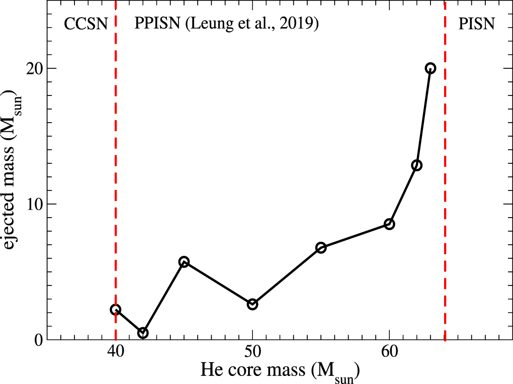
In Leung et al. (2019), we have calculated the evolution of 80–120 M_⊙ stars with metallicities of Z = 10⁻³–1.0 Z_⊙ from the beginning of PPI. Assuming the H-rich envelope is lost, we have further evolved their He cores of 40–62 M_⊙ with Z = 0 through the core collapse. During the pulsation, these He stars undergo extensive mass loss. The ejected masses are 3–13 M_⊙ for 40–62 M_⊙ He stars, as seen in Figure 1, because the pulsations are stronger for more massive He stars (see also Yoshida et al. 2014; Woosley 2017; Marchant et al. 2019). The ejecta form He-rich CSM.

**Figure 1.** Total ejecta mass by pulsation against the progenitor He core mass.
Download figure:
Standard image High-resolution image

The lack of metal lines in the spectra of AT2018cow suggests that the ejecta contains mostly He (Prentice et al. 2018). This feature is consistent with the PPISN model, which ejects mostly the outer layer of the He star during pulsation. (The exact composition can be affected by other stellar parameters, such as the progenitor mass and rotation (Chatzopoulos & Wheeler 2012).

Tolstov et al. (2017) applied a PPISN model of a 50 M_⊙ He star (which is the He core of a 100 M_⊙ star) with a large amount of optically thick CSM (∼20 M_⊙) and kinetic energy of explosion as high as ∼10⁵² erg s⁻¹. They calculated the circumstellar interaction and the resultant light curve. The model explains well the light curve of the Type I SLSN (SLSN-I) PTF 12dam, whose early curve shows a rise of 2.5 mag in 20 days. Such massive CSM is good to reproduce the slow rise of SLSN-I (see also Sorokina et al. 2016), but too massive to explain the fast rise of the light curve of AT2018cow (5 mag in 5 days).

Perley et al. (2019) suggested that in order to reproduce qualitatively the light curve of AT2018cow, there should be a preexplosion ejected mass of ∼0.5 M_⊙. We thus look for in Figure 1 the PPISN model that produces a similar CSM mass. We find that this corresponds to the He star model with the mass M_He = 42 M_⊙. This He star ejects 0.50 M_⊙ of its surface matter, composed of only He, into the surrounding ∼1.6 yr prior to its final collapse.

As seen from the models for SLSNe (Tolstov et al. 2017) and FBOTs (Tolstov et al. 2019), the mass of the optically thick CSM seems to determine the rising timescale of light curves. Based on this, we set here the following working hypothesis that PPISN produces SLSNe if the CSM is massive enough and FBOTs if the CSM is less than ∼1M_⊙.

Based on our working hypothesis, we perform hydrodynamical simulations of the PPISN explosion of a 42 M_⊙ He star. We assume that the He star undergoes core collapse to form a black hole and generates an explosion. With the parameterized explosion energy, we calculate the nucleosynthesis, circumstellar interaction, and bolometric light curves. From the comparison with the observed light curve of AT2018cow, we obtain constraints on the explosion energy, the mixing of radioactive ⁵⁶Ni, the density distribution of CSM, and some other model parameters.

We note that radio and X-ray observations (Margutti et al. 2019) have provided hints that aspherical explosion is necessary for the peculiar evolution of this object. In this work, we use the one-dimensional simulation with spherical approximation to explore which parameters are necessary to reproduce the light curve of this object. We aim to fit the global features of this light curve.

In Sections 2 and 3.1, we review the numerical scheme to calculate nucleosynthesis and the bolometric light curve.

In Section 4, we describe our optimized model, which has a bolometric light curve closest to AT2018cow. We present the detailed evolution of the hydrodynamics and radiative transfer after its explosion.

In Section 5, we present a detailed numerical study to examine the sensitivity of our results on the model parameter and input physics. This includes the explosion energy, ⁵⁶Ni distribution, and CSM properties.

In Section 6, we further discuss how other central energy sources can contribute to or supplement the light curve of AT2018cow. We also discuss how such central energy sources contribute to produce the high-energy photons and compare them with AT2018cow. In the end, we show how our results depend on the radiative transfer code.

2. Initial Model and Methods of Hydrodynamical Simulations

2.1. Presupernova Model

As discussed in the Introduction, we adopt the 42 M_⊙ He star model, which was evolved from the He main sequence to the Fe-core collapse by Leung et al. (2019) through PPI and the associated mass ejection. We used the code MESA (Modules for the Experiments in Stellar Astrophysics, version 8118; Paxton et al. 2011, 2013, 2015, 2017).

In Figure 2, we plot the preexplosion configurations for the density and temperature (top-left panel), velocity (top-right panel), electron mole fraction Y_e (bottom-left panel), and the chemical abundance (bottom-right panel) against M(r), where M(r) is the mass within the radius r. Because the He star has lost 0.50 M_⊙ during PPI, the mass of the collapsing He star is 41.50 M_⊙.

The chemical abundance profile shows three layers. The inner core at M(r) < 2M_⊙, which collapses to a proto-neutron star (and later a black hole), is made up of mostly ⁵⁶Fe. A small fraction of ⁴He exists due to the photodisintegration. A trace of electron-capture products, represented by ⁵⁶Cr,¹⁰ exists in the core, being insignificant at M(r) > 1 M_⊙. The envelope includes an inner envelope and an outer envelope, which differ by their compositions. The inner envelope at M(r) = 2–8 M_⊙ consists of mostly intermediate-mass elements, which feature ²⁸Si and ³²S, and smaller amounts of ³⁶Ar and ⁴⁰Ca. In the outer envelope at M(r) = 8–35 M_⊙, ¹⁶O dominates the composition, with a trace amount of ²⁰Ne and ²⁴Mg. The transition to the outer shell around M(r) ∼ 35M_⊙ can be observed through the emergence of ²⁸Si near the former shock-breakout region during pulsation. The outer shell at M(r) > 35 M_⊙ is mostly ⁴He with a trace amount of ¹²C.

The Y_e profile shows Y_e ∼ 0.46 in the Fe core and a sharp transition to Y_e = 0.5 at M(r) > 5 M_⊙.

The density profile reveals a three-layer structure of the pre-SN: the Fe core at M(r) < 2 M_⊙, the Si–O envelope at M(r) = 2–35 M_⊙, and the outer He shell at M(r) > 35 M_⊙. On the other hand, the temperature profile shows only the core and the envelope structure with no sharp gradient around the He–O interface. The Fe core features a sharp drop of density of five orders of magnitude. The Si–O envelope has a shallow density gradient from 10⁵ to 10³ g cm⁻³. The transition to the outer He shell is shown by the sharp density change. The density also drops sharply toward the surface.

The velocity profile in the Fe core shows homologous contraction at M(r) < 2M_⊙ with a peak velocity at 1.8 × 10⁸ cm s⁻¹. Then, the velocity is zero at M(r) ∼ 5M_⊙. At M(r) > 5 M_⊙, the star is close to hydrostatic.

2.2. Methods of Nucleosynthesis and Radiative Transfer

For the progenitor model as described in Section 2, we first perform the hydrodynamical calculations of nucleosynthesis using the one-dimensional code described in Tominaga et al. (2007). The shock wave is calculated with the PPM method. Nucleosynthesis is calculated with the α network (13 species) coupled with the hydrodynamics and with a big network (280 species) for a post-processing.

For the bolometric light-curve calculation, we use the radiation hydrodynamics code (SNEC; Morozova et al. 2015). The code calculates the transport of blackbody radiation in the diffusion limit to obtain the bolometric light curve. The opacity takes the Rosseland mean opacity mainly from the OPAL tables (Iglesias & Rogers 1993, 1996). The ionization is obtained by solving the Saha equation. For the equation of state (EOS), the Paczynski EOS (Paczynski 1983) is adopted. The gamma-ray heating from the decays of radioactive ⁵⁶Ni and ⁵⁶Co is calculated assuming the gray transfer approximation and pure absorptive opacity.

3. Explosive Nucleosynthesis and Radioactive Heating

3.1. Explosive Nucleosynthesis

For the optimized model in this paper, we set a thermal bomb at the mass cut at M_cut = 2.0 M_⊙ with the internal energy to make a kinetic energy of explosion (hereafter "explosion energy") E = 5 × 10⁵¹ erg s⁻¹. We then calculate the propagation of a shock wave coupled with nucleosynthesis. Nuclear energy release is added to E but is negligibly small.

Figure 3 shows the distributions of the postshock temperature and density at t = 50 s, where t denotes the time after the thermal bomb is deposited. Y_e does not change from the pre-SN values because of the low density in the ejecta.

The core from M_cut to ∼3 M_⊙ contains iron-peak nuclei including mostly ^56–58Ni and ⁴He synthesized in the α-rich freezeout. The middle layer at M(r) = ∼3–10 M_⊙ is occupied by intermediate-mass species including ²⁸Si, ³²S, ³⁶Ar, and ⁴⁰Ca. The inner envelope at M(r) ∼ 10–35 M_⊙ contains mostly light elements mostly ¹⁶O, and then ²⁰Ne and ²⁴Mg. At the surface there are unburned ⁴He and a small fraction of ¹²C. In Table 1, we summarize nucleosynthesis yields of radioactive nuclei at t = 50 s and several species after radioactive decays. In particular, the amount of ⁵⁶Ni is 0.62 M_⊙.

Table 1. The Ejecta Mass and Scaled Abundance Fraction of the Star after Explosive Nucleosynthesis When All Exothermic Nuclear Reactions Have Stopped

Isotope	A	Z	(X_i/⁵⁶Fe)/(X_i/⁵⁶Fe)_⊙	Mass
¹²C	12	6	1.06	1.91
¹³C	13	6	2.11 × 10⁻¹³	4.55 × 10⁻¹⁵
¹⁴N	14	7	1.10 × 10⁻⁸	4.77 × 10⁻⁹
¹⁵N	15	7	5.07 × 10⁻¹⁰	8.72 × 10⁻¹³
¹⁶O	16	8	5.56	22.07
¹⁷O	17	8	7.76 × 10⁻¹¹	1.23 × 10⁻¹³
¹⁸O	18	8	1.12 × 10⁻⁸	1.02 × 10⁻¹⁰
¹⁹F	19	9	2.11 × 10⁻⁹	4.21 × 10⁻¹³
²⁰Ne	20	10	1.88	1.174
²¹Ne	21	10	1.09 × 10⁻⁹	2.17 × 10⁻¹²
²²Ne	22	10	1.24 × 10⁻¹⁰	1.04 × 10⁻¹¹
²³Na	23	11	1.81 × 10⁻⁷	3.36 × 10⁻⁹
²⁴Mg	24	12	3.84	1.04
²⁵Mg	25	12	7.93 × 10⁻⁷	2.86 × 10⁻⁸
²⁶Mg	26	12	2.34 × 10⁻⁵	9.68 × 10⁻⁷
²⁷Al	27	13	3.43 × 10⁻⁴	1.06 × 10⁻⁵
²⁸Si	28	14	10.12	3.52
²⁹Si	29	14	0.517	9.51 × 10⁻³
³⁰Si	30	14	1.11 × 10²	1.39
³¹P	31	15	2.96 × 10⁻⁴	8.05 × 10⁻⁷
³²S	32	16	0.515	0.106
³³S	33	16	2.81	4.75 × 10⁻³
³⁴S	34	16	18.00	0.174
³⁶S	36	16	0.696	2.30 × 10⁻⁵
³⁵Cl	35	17	0.218	3.68 × 10⁻⁴
³⁷Cl	37	17	0.489	2.83 × 10⁻⁴
³⁶Ar	36	18	5.17	0.224
³⁸Ar	38	18	4.73	4.05 × 10⁻²
⁴⁰Ar	40	18	2.30 × 10⁻²	2.48 × 10⁻⁶
³⁹K	39	19	0.151	2.60 × 10⁻⁴
⁴⁰K	40	19	0.213	5.54 × 10⁻⁷
⁴¹K	41	19	1.50	2.00 × 10⁻⁴
⁴⁰Ca	40	20	6.55	0.214
⁴²Ca	42	20	1.06	2.40 × 10⁻⁴
⁴³Ca	43	20	0.257	1.36 × 10⁻⁵
⁴⁴Ca	44	20	2.53	1.94 × 10⁻³
⁴⁶Ca	46	20	2.91 × 10⁻³	3.72 × 10⁻⁹
⁴⁸Ca	48	20	9.04 × 10⁻¹⁰	6.80 × 10⁻¹⁴
⁴⁵Sc	45	21	8.94 × 10⁻²	1.68 × 10⁻⁶
⁴⁶Ti	46	22	0.462	5.45 × 10⁻⁵
⁴⁷Ti	47	22	0.554	6.15 × 10⁻⁵
⁴⁸Ti	48	22	1.99	2.29 × 10⁻³
⁴⁹Ti	49	22	0.418	3.65 × 10⁻⁵
⁵⁰Ti	50	22	0.223	1.93 × 10⁻⁵
⁵⁰V	50	23	7.60	3.13 × 10⁻⁶
⁵¹V	51	23	3.86	6.71 × 10⁻⁴
⁵⁰Cr	50	24	9.26	3.41 × 10⁻³
⁵²Cr	52	24	7.38	5.49 × 10⁻²
⁵³Cr	53	24	2.50	2.16 × 10⁻³
⁵⁴Cr	54	24	0.492	1.08 × 10⁻⁴
⁵⁵Mn	55	25	1.56	1.07 × 10⁻²
⁵⁴Fe	54	26	4.73	0.181
⁵⁶Fe	56	26	1.00	0.623
⁵⁷Fe	57	26	3.26	4.94 × 10⁻²
⁵⁸Fe	58	26	9.29 × 10⁻³	2.16 × 10⁻⁵
⁵⁹Co	59	27	1.41	2.47 × 10⁻³
⁵⁸Ni	58	28	14.74	0.374
⁶⁰Ni	60	28	2.01	2.04 × 10⁻²
⁶¹Ni	61	28	4.70	2.20 × 10⁻³
⁶²Ni	62	28	41.51	6.07 × 10⁻²
⁶⁴Ni	64	28	1.41 × 10⁻⁸	6.29 × 10⁻¹²
⁶³Cu	63	29	0.474	1.50 × 10⁻⁴
⁶⁵Cu	65	29	2.28 × 10⁻⁴	3.34 × 10⁻⁸
⁶⁴Zn	64	30	1.66 × 10⁻²	8.77 × 10⁻⁶
⁶⁶Zn	66	30	1.86 × 10⁻⁶	5.60 × 10⁻¹⁰
⁶⁷Zn	67	30	7.11 × 10⁻⁸	3.29 × 10⁻¹²
⁶⁸Zn	68	30	1.11 × 10⁻⁸	2.38 × 10⁻¹²
⁷⁰Zn	70	30	1.48 × 10⁻⁷	1.09 × 10⁻¹²

Note. All masses are in units of M_⊙. A and Z are the atomic mass and number of the isotopes.

Download table as: ASCIITypeset images: 1 2

3.2. Radioactive Decays and Light Curve

In the adopted PPISN model, the power sources of the optical light curve are circumstellar interaction (Section 4) and radioactive decays of ⁵⁶Ni and ⁵⁶Co. In Figure 5, several theoretical LCs are compared with the observed light curve of AT2018cow (Perley et al. 2019). For the radioactive decay light curve models in Figure 5, we adopt κ_γ = 0.06 Y_e cm² g⁻¹.

(1)
The dashed–dotted purple curve is the bolometric light curve powered by circumstellar interaction only (see Section 4) without radioactive decays. The opacity is calculated for the original abundance distribution (Figure 3). This light curve can reproduce the observed light curve for only the first 20 days.
(2)
The dotted red curve shows the bolometric light curve powered by radioactive decays without circumstellar interaction for the original (centered) distribution of 0.62 M_⊙ ⁵⁶Ni (Figure 3). Its peak luminosity reaches only ∼10^41.5 erg s⁻¹, which is too faint to explain the observations. This implies it takes too long for radioactive heat to reach the surface because of massive ejecta.
(3)
The above comparison suggests that extensive mixing of ⁵⁶Ni to the surface possibly takes place via a jet-like explosion. We thus make the simple assumption that the ejecta is uniformly mixed from the mass cut of M(r) = 2 M_⊙ to the surface of M(r) = 41.60 M_⊙. The uniform abundance distribution is shown in Figure 4. The calculated bolometric light curve is shown by the dashed green curve. Thanks to the ⁵⁶Ni heating in the outer layers, the light curve is consistent with the observations at t > 25 days.
(4)
The solid black curve shows the bolometric light curve with the combined powers of the circumstellar interaction and radioactive decays. A uniform abundance distribution is adopted (Figure 4) to calculate the radioactive heating and opacity. The calculated light curve is in good agreement with the observed light curve of AT2018cow. The later light curve at t > 20 days declines slower than that of AT2018cow, which will be discussed in Sections 4.3 and 5.1. We thus adopt the uniform abundance distribution in Figure 4 for the model we call the "optimized" model.

**Figure 4.** The abundance pattern of the ejecta and CSM adopted in the optimized model (see next plot). The ejecta is assumed to be completely mixed as a representation of aspherical explosion.
Download figure:
Standard image High-resolution image

4. Circumstellar Interaction

4.1. Formation and Structure of Circumstellar Matter

In calculating the light curve powered by circumstellar interaction, we adopt the He star model of M_He = 42.10 M_⊙, which undergoes PPI and ejects He-rich surface materials to form CSM of mass M_CSM = 0.50M_⊙ ∼1.6 yr prior to its collapse (see the Introduction). Thus, the He star has M_He = 41.60M_⊙ at the beginning of Fe-core collapse.

We plot in Figure 5 the bolometric light curve using the chemical distribution shown in Figure 4. We also present contrasting models to demonstrate the individual contributions of CSM and the decay-chain of ⁵⁶Ni. We assume that the CSM has a constant density of ρ_CSM = 10⁻¹¹ g cm⁻³ extending to R_CSM ∼ 10¹⁴ cm as seen in Figure 6. Note that such CSM is optically thick. We examine in Section 5 how the shape of the bolometric light curve depends on M_CSM, ρ_CSM, and R_CSM, and how the comparison with AT2018cow provides constraints on these quantities.

**Figure 6.** The stellar and CSM density profiles of the initial models. The black solid line shows the optimized model. Other lines show those for the comparisons in Section 5. All models have the same CSM mass M_CSM = 0.50 M_⊙ and an outer CSM radius R_CSM ∼ 10¹⁴ cm.
Download figure:
Standard image High-resolution image

Spectroscopic observations of AT2018cow have reported the appearance of H features in the spectra ∼15 days after the light maximum (Perley et al. 2019). The existence of some H in the ejecta and CSM can be explained as follows. During the evolution, the progenitor star of the PPISN loses a large fraction of its massive H envelope (e.g., Leung et al. 2019). The exact amount of H that remains in the progenitor depends strongly on the mass, metallicity, and binarity of the progenitor. If some amount of H remains in the star when the mass ejection due to PPI occurs, the CSM of the PPISN contains some H.

Another possibility for why some H exist in the CSM is the case where a H-rich environment has been formed outside the progenitor star. During the ejection of the He envelope due to PPI, the high-velocity He shell may interact with the surrounding low-velocity H-rich materials. The deceleration of the He shell causes Rayleigh–Taylor instabilities, and some H-rich matter is mixed into the He shell.

We also examine in Section 5 how the existence of H affects the light-curve shape.

4.2. Hydrodynamical Evolution of the Shock Propagation

We start the radiation hydrodynamical simulation from the Fe-core collapse. A shock wave is generated by inserting a thermal bomb with explosion energy E = 5 × 10⁵¹ erg at the mass cut M_cut = 2 M_⊙. The elemental abundance profile obtained from the explosive nucleosynthesis calculation (Figure 3) is assumed to be uniformly mixed (Figure 4).

In Figure 7, we plot the distributions of the density (top-left panel), velocity (top-right panel), temperature (middle left), free-electron fraction (middle right), optical depth (bottom left), and luminosity profile (bottom right) for the optimized model at Days 0 (solid black line), 1 (red dotted line), 5 (green dashed line), 10 (blue long-dashed line), 20 (purple dotted–dashed line), and 30 (cyan dotted–long-dashed line) after the formation of the shock wave. Here, CSM at $M(r)=41.6-42.1\,{M}_{\odot }$ is included.

Density (ρ): The initial density profile is the precollapse profile shown in Figure 2 and the 0.50 M_⊙ CSM with a constant density of 10⁻¹¹ g cm⁻³ extending to ∼10¹⁴ cm as seen in Figure 6. We note that the CSM is optically thick. At Day 1, the shock wave has arrived at the inner radius of the CSM and enhanced the density there by two orders of magnitude. At Day 2, the shock breakout from the CSM occurs. At Day 5, the postshock structure develops with a trough inside the inner CSM and a bump just behind the CSM. A reverse shock can be seen around Day 10, but it freezes when the free expansion of matter dominates the motion.

Velocity (v): When the shock wave arrives at the CSM on Day 1, the velocity at the inner edge of the CSM reaches as high as 1.4 × 10⁹ cm s⁻¹, while the outer part of the CSM is close to static. During the propagation, the shock wave transfers its momentum to the CSM as seen in the profile at Day 3. Because of the much smaller mass, the CSM reaches a velocity of 1.5 × 10⁹ cm s⁻¹ which is much higher than the 8 × 10⁸ cm s⁻¹ in the He star. Most of the star has already developed homologous expansion after Day 5, except for a small nonvanishing reverse shock near the inner boundary of the CSM.

Temperature (T): The compact precollapse He star has a surface temperature as high as ∼10⁷ K. The CSM is assumed to be isothermal at 10⁴ K. When the shock wave reaches the inner boundary of the CSM at Day 1, the surface temperature has already cooled down to <10⁵ K, while the shock-heated matter can be as hot as 2 × 10⁵ K. At Day 5, the hot temperature bump smears out due to diffusion. Around Day 20, both the star and CSM become isothermal.

Free-electron fraction (X_e): X_e is an important factor for the opacity as a free electron has a small but constant cross section, compared to other bound–free and bound–bound transitions, which strongly depend on the population of particular ionization stages. At the beginning, the star is completely ionized, while the CSM is less ionized with a fraction of ∼40%. Once the shock wave reaches the surface, the heat allows the rapid ionization of the CSM. At Day 5, when the reverse shock is propagating backward, the matter near the outer layer of the star has a low-enough density and temperature for recombination. At Day 10, the recombination region is more extended. The shock-heated front remains fully ionized, but the whole profile is bumpy, because of the shock-induced density fluctuations. At Day 20, when the photosphere starts to recede, the CSM cools down and more matter has recombined. At Day 30, the whole ejecta gradually recombines.

Optical depth (τ): Initially, the star and CSM are opaque, having τ > 1 except at the very shallow layer just below the stellar surface. As the star expands, τ decreases. However, the shock front makes the opacity sufficiently high that the photosphere remains at the outermost part of the star. By Day 20, the photosphere gradually retreats to M(r) ∼ 40 M_⊙. At Day 30, the photosphere has receded much deeper into the star, showing that the ejecta gradually becomes transparent.

Luminosity (L(r)): When the shock starts to interact with the CSM, the luminosity profile becomes extremely bumpy because of the fluctuations of the temperature, density, free-electron fraction, and thus opacity because of shock propagation. At Days 3 and 5, the stellar surface becomes the brightest part of the star. However, a trough in the luminosity develops when the reverse shock allows an early recombination of atoms. Beyond Day 20, the luminosity profile has reached a steady state where radiation develops steadily and reaches a uniform luminosity at Day 30. The photosphere recedes by ∼1 M_⊙ every 10 days.

4.3. Radiation Hydrodynamical Results

In Figure 8, we plot the radiation hydrodynamical results of our "optimized" model, i.e., the bolometric luminosity (top-left panel), effective temperature (top-right panel), photospheric radius (bottom-left panel), and velocity at the photosphere (bottom-right panel). The solid lines show the model with circumstellar interaction as described in the earlier subsection. When the shock breakout from the optically thick CSM occurs at Day 2, the bolometric luminosity reaches a bright peak. Then, the luminosity rapidly declines through radiative cooling. Such a sharp rise to a bright peak and a rapid decline of the light curve well reproduce the observed FBOT-like feature of AT2018cow (Perley et al. 2019). After Day 18, the luminosity would decrease too rapidly if there were be no radioactive heating, as already shown in Figure 5.

For comparison, the results for the model without CSM are shown by the dashed curve. There is no sign of shock breakout where the light curve is smooth and flat. Its luminosity around Day 2 is almost three orders of magnitude lower than the peak due to circumstellar interaction, but it reaches an asymptotic value of ∼10⁴² erg s⁻¹ at Day 20.

Then, the bolometric light curve produced by the combined powers of the circumstellar interaction and radioactive decays shows a good agreement with AT2018cow. The effect of shock-heated CSM is seen in the luminosity evolution.

However, the observed temperature and radius at the photosphere of AT2018cow monotonically decrease (Perley et al. 2019), which suggests that the photosphere recedes inward in M(r) at a pace different from the model. Such a difference in the local quantities at the photosphere might stem from a possible aspherical structure of the CSM and the ejecta of AT2018cow. It would be interesting to investigate the radiation hydrodynamics of a multi-D structure of CSM–ejecta.

4.4. Spectral Evolution of AT2018cow

Although we focus on mainly reproducing the evolution of the bolometric flux from AT2018cow, our optimized model also broadly outlines some aspects of its spectral evolution (Prentice et al. 2018; Perley et al. 2019).

According to the observations, the spectra of AT2018cow are very blue and almost featureless in the beginning, for Days 4 to 8 after the maximum (Perley et al. 2019), which roughly corresponds to Days 7 to 11 after the explosion. This is exactly what we expect to see in our optimized model. The optical depth in Figure 8 shows that on Day 10, the photosphere is located in the outermost layers of CSM. These layers are shock-heated to about 20,000 K at this time. The continuum emission must be very bright under such conditions, and optical lines, even if some of them were formed at very high temperature, sink below the continuum level.

Between Days 10 and 20, the photosphere starts to dive back into the ejecta layers, while the temperature falls down to 9000–10,000 K. The conditions become more suitable for forming optical lines, and exactly during this period, they appear in the spectrum of AT2018cow.

The problem arises with the explanation of the weak narrow components of lines that are often observed after Day 20 in the spectra of AT2018cow. These lines do not appear in the ejecta and CSM of the optimized model, because all materials in the model are already accelerated to velocities as high as 7000–13,000 km s⁻¹. But these weak components do not resemble the typical shape of the lines of Type IIn SNe (SNe IIn). These are much weaker than in SNe IIn. We suppose that these weak lines must not arise from the spherical envelope, into which the exploding object is embedded, as it happens in SNe IIn. Instead, these lines can be emitted, for example, by more extended nearby (possibly a disk-shaped) structure lost by the progenitor much earlier, having low velocity and illuminated by the explosion.

The late appearance of hydrogen lines (Perley et al. 2019) is expected from such extended CSM with hydrogen that was lost earlier (Section 4.1). As will be shown in Section 5.5 and Figure 6, when we admix a large amount of hydrogen into the helium CSM, this affects the bolometric light curve very weakly.

5. Dependence of the Light Curve on Model Parameters

5.1. The Comparison Model

In the previous section, we have studied how the combined powers of circumstellar interaction and radioactive decays can explain the bolometric light curves of AT2018cow and obtained the "optimized" model.

We should note that the theoretical bolometric light curve depends on a number of parameters and assumptions adopted in the modeling. Here, we study how the light curves depend on the choice of these parameters.

For these comparison studies, we construct a "comparison" model whose bolometric light curve is in fairly good agreement with AT2018cow but with a different set of model parameters from the "optimized" model. In this "comparison" model, the elemental abundance distribution in Figure 9 is assumed. Here, the original abundance distribution is adopted to calculate the equation of state and opacities except for radioactive ⁵⁶Ni, which is moved to the outer layers at M(r) = 9.0–41.6 M_⊙. The aim is to study the enhanced heating effects of ⁵⁶Ni by mimicking the jet-like ejection of the ⁵⁶Ni-rich region from a deeper layer.

**Figure 9.** The abundance distribution adopted in the "comparison" model used for the parameter study in this section. It assumes that only radioactive ⁵⁶Ni is brought to the outer layers of M(r) = 9.0–41.6M_⊙.
Download figure:
Standard image High-resolution image

In Figure 10, the bolometric light curve for this "comparison" model is shown by the black solid line compared with the observed data of AT2018cow (Perley et al. 2019). For radioactive heating, the "comparison" model (black solid line) adopts a ${\kappa }_{\gamma }=0.06\,{Y}_{{\rm{e}}}$ (ρ/ρ₀)cm² g⁻¹ if ρ < ρ₀ = 10⁻¹⁰ g cm⁻³. If the constant γ-ray opacity κ_γ = 0.06 Y_e cm² g^–1 is adopted, the light curve is shown by the red dotted line, whose decline is too slow to be compatible with AT2018cow. The reduction of κ_γ at low densities could mimic the effects of clumpy density distribution (e.g., Equation (1) of Kumagai et al. 1989) in the ejecta. Because the black solid curve is in better agreement with the late-time data of AT2018cow, we treat this "comparison" model as a default model for comparison.

5.2. Dependence on Explosion Energy

In the light-curve calculation, we treat the kinetic energy of the explosion E as a model parameter. Theoretically, the explosion mechanisms of core-collapse SNe are not well understood. Thus, it is not certain how much explosion energy is given to the ejecta. For example, if a black hole is formed with an accretion disk around it, a powerful bipolar jet from magnetohydrodynamical instabilities may provide a large amount of energy to the ejecta. Without actual modeling of a core-collapse SN, it would be useful to constrain the explosion energy from the light-curve modeling. Here we examine how the light curve depends on the explosion energy. We thus search the explosion energy from E = 10⁵¹ to 10⁵² erg, which produces the closest light curve to AT2018cow.

In Figure 11, we plot the light curves for the comparison model with explosion energies of E = 2.5 × 10⁵¹, 5 × 10⁵¹, and 10⁵² erg, respectively. Other parameters, such as the CSM profile and the resolution, are the same as in the comparison model. It is seen that the effects of the explosion energy are secondary. It does not play an important role in the shock-breakout time and the peak luminosity. It affects a little the postmaximum decrease and the fluctuations of the luminosity. The model with higher explosion energy fades slower, because the stronger shock makes the postshock density higher, thus making the recession of the photosphere slower.

5.3. Dependence on CSM Structure

The comparison model is assumed to have CSM with a constant density of 10⁻¹¹ g cm⁻³. Here, we examine how the light curve depends on the CSM density structure by adopting a profile of 1/r^α with α = 0, 1, and 2, as shown in Figure 6. In constructing the density profile, we require that the CSM has the same mass ∼ 0.5 M_⊙ and the same outer radius as the comparison model.

In Figure 12, we plot the light curves for the comparison model (black solid) and its variations with different CSM density profiles: i.e., 1/r (red dashed line) and 1/r² (green dotted–dashed structure). It is seen that, qualitatively, the light curve is not sensitive to the CSM density profile. The steeper CSM density results in a quicker decrease in the luminosity and a lower luminosity peak. The late luminosity evolution becomes very close to each other and overlaps when the ⁵⁶Co decay dominates the light curve.

5.4. Dependence on CSM Density

Here we examine the dependence on the CSM density ρ_CSM.

We take the total mass of the CSM to be the same as the comparison model, and we vary the inner and outer boundaries of the CSM as two model parameters. In Figure 13, we plot the initial structure of the comparison model and those with the various CSM density from 10⁻¹¹ to 10⁻⁹ g cm⁻³. For a higher ρ_CSM, the outer radius of the CSM can be almost an order of magnitude smaller than the model with a lower ρ_CSM.

**Figure 13.** The initial stellar and CSM density profiles of the models comparing the effects of the CSM density. All models have the same CSM mass 0.5 M_⊙ and a flat CSM profile.
Download figure:
Standard image High-resolution image

In Figure 14, we plot the corresponding light curves for the explosion models assuming the same explosion energy of 5 × 10⁵¹ erg and the same resolution of the mass grid, 0.04 M_⊙, as the comparison model. The CSM density plays an important role in two aspects.

(1)
First, the initial peak (shock breakout) depends sensitively on ρ_CSM and hence the outer radius of CSM. The first peak changes from Day 3 to Day 1 when ρ_CSM increases from 10⁻¹¹ to 10⁻⁹ g cm⁻³, which corresponds to the decrease in the CSM outer radius from 3 × 10¹⁴ cm to 5 × 10¹³ cm.
(2)
Second, the postpeak evolution before the ⁵⁶Co decay is sensitive to ρ_CSM. For lower ρ_CSM, the postpeak fall in the luminosity is faster. It takes about 5 days for the comparison model (ρ_CSM = 10⁻¹¹ g cm⁻³) to decrease one order of magnitude in luminosity, compared to the one with higher ρ_CSM = 10⁻⁹ g cm⁻³, for which it takes about 10 days for the luminosity to decrease by one order of magnitude.

5.5. Dependence on Hydrogen in the CSM

In the spectra of AT2018cow, H features appear ∼15 days after the light maximum (Perley et al. 2019). We then discuss in Section 4.1 the formation scenario that has some H in the ejecta and CSM.

To examine the possible effects of H in the CSM, we approximate the composition of the CSM from pure He to two other abundances: low H mixing (0.1 H and 0.9 He) and high H mixing (H and He are 50% by mass fraction).

In Figure 15, we plot the corresponding light curve with the data point from COW. The light curves are almost identical despite the photosphere still lying inside the CSM. The model with the higher H mixing has a slightly lower bolometric luminosity at Day 18 despite a similar light-curve shape. The effects of H only become observable in the H-rich model, which shows a higher luminosity at Days 28–30.

5.6. Dependence on CSM Mass

The mass of the CSM M_CSM depends on the dynamical mass loss during PPI, thus being sensitive to the progenitor mass. Here we examine how the light curve depends on M_CSM for the same R_CSM as the comparison model.

In Figure 16, we plot the light curves for three models with M_CSM/M_⊙ = 0.50 (black solid line for the comparison model), 1.0 (red dotted line), and 2.0 (green dashed line), having the same R_CSM.

The light-curve features depend strongly on M_CSM. Larger M_CSM delays the shock breakout of the light curve from Day 2 to about Day 3. The peak luminosity is also higher for larger M_CSM. The declining slope of the light curve becomes flatter when M_CSM is large. For M_CSM = 2.0M_⊙, the light curve remains ∼10⁴⁴ erg s⁻¹ between Day 5–25. As a result, the transition to the phase powered by ⁵⁶Co decay is also slightly delayed. These trends are the effects of a longer diffusion time in more massive CSM.

Our results confirm that M_CSM is strongly constrained by the light-curve width and as small as ∼0.5M_⊙, consistent with AT2018cow as Perley et al. (2019) has estimated.

5.7. Dependence on Resolution

How the shock propagates through the CSM controls the early evolution of the light curve. That means how the shock is resolved is important to trace how the kinetic energy of the shock is transformed to the internal energy and hence the blackbody radiation through shock compression. Here we examine how the results depend on the choice of the resolution.

In Figure 17, we plot the light curves of the comparison model with the current resolution (1000 grids), two times and four times higher resolutions. The highest resolution has a mass resolution of ∼10⁻² M_⊙. The qualitative features of the light curve are very well captured from the current resolution. The higher resolution has a higher maximum luminosity in the early peak, owing to the smaller mass shell. After the shock breakout, three models behave similarly, except at Day 20, when the bump appears later because the resolution is lower. Despite that, the similarity of the three light curves shows that the shock propagation is already well captured by the current resolution.

5.8. Comparison with STELLA

In this subsection, we compare the numerical results with the multicolor radiative transfer calculation done by the code stella (Blinnikov et al. 2006; Baklanov et al. 2015). In the bulk of the present work, we did not use stella because its implicit and multiband nature makes searching for the parameters for the optimized light curve unavoidably time-consuming.

Here we compare our results obtained from the blackbody diffusion-limit radiative transport calculation by snec with the results computed by stella. We give comparisons only for the bolometric light curve of the comparison model described in Section 5.1. The multiband light curves calculated by stella for another set of models are presented in a separate publication (E. Sorokina et al. 2020, in preparation).

The pre-SN model calculated by MESA has more than 1200 mesh zones. Blue dots in Figure 18 show that our remapping of this model for stella runs with 232 zones, which is much more uniform than the one used for snec. It is clear that the resolution of the structure in the interior is sufficiently high.

Both the stella and snec codes are spherically symmetric, Lagrangian, radiation-hydrodynamic ones. Hydrodynamics equations embedded in the stella and snec codes are quite similar. The principal differences between the codes are in the implementation of radiative transfer into hydrodynamical simulations. stella solves implicitly time-dependent equations for the angular moments of intensity in fixed frequency bins which are coupled with the Lagrangian hydrodynamical equations. Therefore, there is no need to ascribe any temperature to the radiation, thus the photon energy distribution may be quite arbitrary. snec uses the equilibrium-diffusion approximation for radiation transport. Thus, a blackbody spectrum is enforced in snec with the same temperature for radiation and matter.

In the snec model, the photosphere is located in the outer layers during the first 35 days, and the blackbody approximation is quite applicable to the reconstruction of the bolometric light curve. Figure 19 demonstrates a reasonably good agreement of the bolometric fluxes of snec and stella for this period.

**Figure 19.** Bolometric light curves adopted by snec (thin line) and stella (dotted blue line) for the pre-SN models shown in Figure 9.
Download figure:
Standard image High-resolution image

We observe that the two codes agree qualitatively well. The two models can produce the rapid rise of AT2018cow within the first 3–4 days. Later, the luminosity in stella falls a bit faster due to faster recombination in the outer layers with the mass ∼2 M_⊙ from the edge of the ejecta which are above the photosphere at this epoch. Given many differences in the treatment of opacity and radiative transfer in snec and stella, we find that the agreement is satisfactory. Understanding the effect on light curves of different approaches in the snec and stella codes requires a detailed comparative study (E. Sorokina et al. 2020, in preparation).

Note that stella calculates both the effective temperature T_eff and the color temperature T_color. At the shock breakout, T_color reaches ∼10⁶ K, which is much higher than the T_eff ∼ 10⁵ K obtained by snec.

6. Discussion

In the previous sections, we have shown that the FBOT-like feature of the early bolometric light curve of AT2018cow is reproduced well by circumstellar interaction in our optimized model before Day 20. After Day 20, the bolometric light curve is modeled well by radioactive decays, but it requires extensive mixing of ⁵⁶Ni almost uniformly up to the ejecta–CSM interface. Thus, it is still worth discussing other possible central energy sources to power the late light curve in our PPISN model.

6.1. Fallback onto the Black Hole

The progenitor of a PPISN is as massive as 80–140 M_⊙; thus, it is likely that a black hole is formed in the center. It is possible that fallback of matter onto the black hole occurs to provide a late-phase energy source other than the ⁵⁶Ni decay or circumstellar interaction. In view of that, we include the fallback energy source in the comparison model. In our spherical explosion model, where we insert an energetic thermal bomb, no direct fallback occurs, so we use a parameterized fallback formula.

We adopt the analytic formula for energy deposition (Michel 1988; Chevalier 1989; Dexter & Kasen 2013)

$\begin{eqnarray}&&\dot{\epsilon }=A/{M}_{\mathrm{dep}}{t}^{-2.5},\end{eqnarray} \tag{ 1 }$

where A is a parameter for the energy-deposition rate, and M_dep is estimated from the photon mean free path. However, the compact inner core leads to energy deposition focused on the innermost shells for most of the time. A is determined by how much mass is accreted during the simulation. The new model has two energy sources: one is the decay of ⁵⁶Ni and the other is the fallback.

In Figure 20, we plot the light curves for the two models and find that the two light curves overlap with each other. This is expected because, in the early light curve, the photosphere is located in the CSM or in the outer ejecta. The energy from the fallback has indeed modified the internal structure of the core by thermal expansion. However, the timescale for the energy to arrive at the photosphere depends on the diffusion timescale. As a result, no significant change can be seen in the model with the fallback energy deposition.

However, we remark that multidimensional modeling of fallback can be very different from one-dimensional modeling. The jet structure may form when the progenitor rotates. The rotating black hole accommodates a rapidly rotating accretion disk, where the gravitational instability in the disk after the formation of a dead zone can trigger large-scale mass and energy ejection (see, e.g., Tsuruta et al. 2018). In a multidimensional model (see, e.g., Tominaga et al. 2007), the jet can break out and form two holes. This drastically reduces the site of the fallback onto the black hole to the photosphere. To reproduce this phenomenon, we need to parameterize the energy-deposition depth into the outer ejecta.

6.2. Magnetar Model

We do not consider a magnetar (Kasen & Bildsten 2010; Kasen et al. 2016) as a power source for the late light curve in the present PPISN model because of the following reasons.

(1) The progenitor of the PPISN is so massive as 80–140 M_⊙ that it may not form a neutron star remnant. (2) Even if we assume the formation of a magnetar in our PPISN model, the diffusion time for the magnetar energy to reach the photosphere would be too long to explain the observed light curve after Day 18, being similar to the black hole accretion model shown in Figure 20.

Note, however, that the magnetar activity may form a jet-like ejecta. The magnetar, which loses energy through its dipole radiation, can effectively transfer its energy by electromagnetic waves along the confined angle. Such a jet-like structure might reduce the timescale to transfer the magnetar energy to the surface.

If the progenitor of AT2018cow were a much smaller star, however, it may not encounter the above two problems (e.g., Fang et al. 2019). In such a low-mass model, we need CSM to power the early light curve to reproduce the FBOT-like feature. Actually, the super-AGB progenitor of the electron-capture SN forms such a CSM as well as a neutron star, and that is the model applied for the FBOT KSN 2015K by Tolstov et al. (2019). Such a case would be worth investigating for a model of AT2018cow (E. Sorokina et al. 2020, in preparation).

6.3. High-energy Photons of AT2018cow

In Margutti et al. (2019), the detailed X-ray and gamma-ray light curve and spectra of AT2018cow are presented.

Here we discuss how the possible energy source of the light curve of AT2018cow (circumstellar interaction, magnetar, and accreting BH) can be related to the detected X-ray.

In the circumstellar interaction model, the shock-heated matter has the "color" temperature as high as ∼10⁶ K according to the calculation of stella as mentioned in Section 5.8. Such high-temperature materials emit X-rays, which may easily escape from the star.

If the aspherical explosion is the case illustrated in Figure 2 of Margutti et al. (2019), the ejecta near the "equator" can be ejected faster and is less compact than those near the "poles." The formation of aspherical CSM allows time to lapse for the interaction to take place.

When a bipolar-like explosion takes place, the two poles are more readily penetrated by the high-velocity flow. Depending on the jet energetics, the jet can break out directly on the surface and trigger the X-ray burst by the interaction.

If aspherical explosion occurs, the bipolar structure forms as discussed in an earlier subsection for the accreting black hole and magnetar and allows early X-ray emission.

When the shock breakout occurs, it creates an opening of the star reaching the compact core directly. The high-energy photon coming from the black hole or neutron star can escape the star efficiently.

The exact nature of the aspherical explosion and its early high-energy photon emission (see Figure 12 of Margutti et al. 2019) will require multidimensional radiative transfer simulations to understand, which will be an interesting future project.

7. Conclusion

In this work, we apply the model of circumstellar interaction in a PPISN to explain the FBOT AT2018cow (COW). AT2018cow has quite a unique early light curve, showing a peak as bright as that of SLSNe but a much faster rise and fall than SLSNe. We apply the evolutionary model of a 42 M_⊙ He star which collapses after undergoing PPI mass ejection, and compute the corresponding bolometric light curves. We have searched for optimized model parameters (explosion energy, CSM density and structure, and distribution of ⁵⁶Ni) with which the bolometric light curve of AT2018cow is well reproduced.

We show that an explosion of a PPISN with energy ∼5 × 10⁵¹ erg, ⁵⁶Ni mass of ∼0.6 M_⊙, CSM mass of 0.5 M_⊙, and density of 10⁻¹¹g cm⁻³ produces an optimized model whose bolometric light curve is in best agreement with AT2018cow.

We also studied how each model parameter affects the light curve. We note that the simulation reaches the convergence regime in the resolution (mass shell ∼2 × 10³¹ g). The explosion energy plays a secondary role in the light-curve shape. On the other hand, the CSM mass, density, and structure dominate the light-curve shape. Mixing of ⁵⁶Ni is necessary to explain the slow decline of the luminosity beyond Day 20. Observable differences in the photosphere evolution suggest that further validations are necessary to connect the FBOT AT2018cow to the PPISN model.

To explain the late-time light curve and the high-energy photon after shock breakout, a central engine such as fallback onto a black hole or a magnetar remains important. Despite that, the interaction can still provide the necessary condition for the rapid rise and drop of the light curve up to ∼40 days. Further discrimination of models will require multidimensional simulations to trace how the aspherical energy deposition contributes to the high-energy photons detected.

Based on our successful model for FBOT (AT2018cow) with the CSM mass of 0.5 M_⊙ and the model for SLSN (Tolstov et al. 2017) with the CSM mass of ∼ 20M_⊙, we set the following working hypothesis that PPISNe produces SLSNe if the CSM is massive enough and FBOTs if the CSM is less than ∼1M_⊙.

This work was supported by World Premier International Research Center Initiative (WPI Initiative), MEXT, Japan, and JSPS KAKENHI grant Nos. JP17K05382 and JP20K04024. K.N. would like to thank Brian Metzger and Raffaella Margutti for useful discussion at the UCSB/KITP program "The New Era of Gravitational-Wave Physics and Astrophysics" in 2019. S.C.L. thanks the MESA development community for making the code open source and V. Morozova and her collaborators in providing the snec code open source. S.C.L. acknowledges support by funding HST-AR-15021.001-A and 80NSSC18K1017. S.B. is sponsored by grant RSF 19-12-00229 in his work on supernova simulations with the stella code. P.B.'s work on understanding the effect on light curves of different approaches in the SNEC and stella codes is supported by the grant RSF 18-12-00522. E.S. is supported by the grant RFBR 19-52-50014 in her work on developing codes modeling the radiative transfer in supernovae.

Software: MESA (v8118; Paxton et al. 2011, 2013, 2015, 2017), SNEC (Morozova et al. 2015), stella (Blinnikov et al. 2006; Baklanov et al. 2015).

A Model for the Fast Blue Optical Transient AT2018cow: Circumstellar Interaction of a Pulsational Pair-instability Supernova

Article metrics

Permissions

Author e-mails

Author affiliations

ORCID iDs

Dates

Abstract

1. Introduction