


Abstract
We employ data from the 2019 Magnetospheric Multiscale (MMS) Solar Wind Turbulence Campaign to evaluate scaling and anisotropy of second-order magnetic field structure functions and scale-dependent kurtosis from a single data interval. Prior results have been based either on the Taylor approximation, which conflates time and space dependence, or on averaging many data sets, which introduces sample-to-sample variation of plasma parameters. The present results overcome these systematic effects. We find that for length scales between 57 and 201 km the fluctuations are anisotropic with a preferred orientation of 60°–70° to the magnetic field direction. The peak kurtosis also lies in this angular range. This confirms anisotropy of the spectrum and suggests that coherent structures such as current sheets are oriented nearly perpendicular to the magnetic field direction. Both the anisotropy and the kurtosis decrease approaching the ion inertial length, here ≈91 km.
Export citation and abstract BibTeX RIS
1. Introduction
Two important features of turbulence in the solar wind are the distribution of fluctuation energy over length scales (Matthaeus & Goldstein 1982; Alexandrova et al. 2013), and higher-order fluctuation statistics such as kurtosis (Bruno et al. 1999; Hada et al. 2003; Matthaeus et al. 2016), and the anisotropy of these measurements with respect to the direction of the magnetic field (Dasso et al. 2005; Osman & Horbury 2009). These statistical properties are influential in many applications and in fundamental theories (Jokipii 1973; Oughton et al. 2015). Examples include theories of heating due to cascade or due to mechanisms such as reconnection, cyclotron resonance, or kinetic Alfvén waves (Isenberg & Hollweg 1983; Hollweg 1999; Leamon et al. 2000), as well as processes related to particle scattering, magnetic field line connectivity, and field line random walk. The usual procedure of such studies has been to evaluate the relevant turbulence quantities through familiar approximations, especially the Taylor hypothesis (Taylor 1938; Jokipii 1973; Matthaeus & Goldstein 1982). Increase in availability of simultaneous multispacecraft measurements has, in recent years, afforded alternative strategies, usually at a single scale (or very similar scales in a tetrahedral formation) for each interval sampled (Weygand et al. 2006; Osman & Horbury 2007; Horbury et al. 2012; Chhiber et al. 2018). While tremendous advances have been made using these methods, there are inherent limitations (Klein et al. 2019; Matthaeus et al. 2020). Here we will employ a different strategy, based on simultaneous collinear measurements that span more than a decade of spatial lags in solar wind turbulence. This analysis is made possible in a novel formation of the four Magnetospheric Multiscale (MMS) spacecraft (Burch et al. 2016) that was obtained as part of the special Solar Wind Turbulence Campaign in 2019 February. Using these data we compute the turbulent magnetic field amplitude, and the scale-dependent kurtosis, each as a function of scale and angle to the local magnetic field. The results span more than a decade of length scale near the ion inertial scale, and are obtained from a single 5 hr period of solar wind data, making use of none of the usual approximations.
Typically solar wind turbulence studies estimate quantities such as turbulence energy distributions, as measured by spectra, or equivalently second-order structure functions, or scale-dependent kurtosis, the normalized fourth-order moment. The standard procedure invokes the Taylor hypothesis (Jokipii 1973), whereby the measurements based on a time lag may be interpreted as related to a spatial lag, using the rapid flow of plasma and the mean solar wind speed, as a fixed proportionality constant in each interval. To obtain information about anisotropy of the underlying turbulence statistics, the Taylor approximation approach has been employed for analysis relative to a fixed large-scale average magnetic field, or relative to average magnetic field obtained by some form of averaging (Chen et al. 2011). An important but less available alternative is one that does not employ the Taylor hypothesis, but makes use of pairs of spacecraft to derive two-point, single time statistics at a single scale—set by the spacecraft separation. This variation avoids issues with time variation during a measurement, but usually requires the use of a large number of different solar wind intervals to obtain data on anisotropy or even variation of correlation over a significant range of length scale separations.
2. 2019 MMS Turbulence Campaign
In the special MMS Solar Wind Turbulence Campaign, in 2019 February, the four MMS spacecraft were rearranged into a "beads on a string" configuration instead of the standard tetrahedron formation. The four spacecraft were positioned in a collinear configuration with log-spaced separation. Interspacecraft separations ranged from 30 to 200 km. Additionally, the spin axis was tilted to obtain improved electric field measurements. In this phase of the MMS orbital parameters, the formation spent a substantial period of time during each orbit in the solar wind, well beyond the bow shock. As such, the project was able to obtain a number of useful burst resolution measurements in the solar wind. The longest of those was a continuous interval of burst data lasting 5 hr, and which is analyzed in this paper, as well as in Bandyopadhyay et al. (2020). For orientation, the configuration of the four MMS spacecraft, while in the solar wind during the Turbulence Campaign, is illustrated in Figure 1.
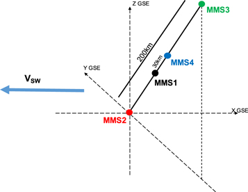
Figure 1. Diagram of the configuration of the four MMS spacecraft near apogee, during the turbulence campaign. Note that close to apogee, when the spacecraft are in the pristine solar wind, they are aligned on the GSE Y–Z plane perpendicular to the solar wind flow.
Download figure:
Standard image High-resolution image3. MMS Data
We employ 5 hr of magnetic field data from the Fluxgate Magnetometer (FGM; Russell et al. 2016) on board each each of the four MMS spacecraft. These are designated as MMS1, MMS2, MMS3, and MMS4. The magnetic field data are accumulated at a resolution of 128 Hz and synchronized across the formation. The orbital context is illustrated in the top panel of Figure 2. The middle panel of Figure 2 shows the three Geocentric Solar Ecliptic (GSE) components of magnetic field recorded in this period by the MMS1 spacecraft.
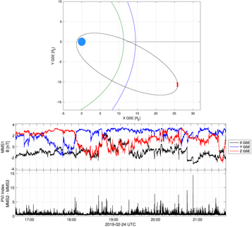
Figure 2. Top: location of the MMS spacecraft during this interval in bold red, along with the orbit in black. The magnetopause and bow shock are shown in light green and light blue, respectively, as estimated from OMNI data. Bottom: time series of magnetic field and PVI as defined in Equation (1), for the 5 hr interval in the solar wind. Several structures at MHD and kinetic scales (flux tubes, current sheets) can be seen.
Download figure:
Standard image High-resolution imageTo visualize and quantify the roughness or intermittency of the magnetic field signal, we compute the partial variance of increments (PVI) of the magnetic field for this interval. The PVI, which can be computed either with two spacecraft or with a single spacecraft and the Taylor hypothesis (Chasapis et al. 2015; Greco et al. 2018) is defined as
where here, for the multispacecraft case, the spatial lag  , for the position of MMS spacecraft number I given by
r
I
, so that that the vector increment is
, for the position of MMS spacecraft number I given by
r
I
, so that that the vector increment is  . The lower panel of Figure 2 shows the time series of the values of PVI computed in this way (Chhiber et al. 2018; Greco et al. 2018), namely, the two-point PVI value using spacecraft MMS2 and MMS3. The separation between these two spacecraft is ∼200 km, which corresponds to ∼2di
. The sharp reversals of the magnetic field as well as the the peaks of the PVI shown in Figure 2 indicate the presence of several structures at both MHD and kinetic scales, as is typical for solar wind turbulence.
. The lower panel of Figure 2 shows the time series of the values of PVI computed in this way (Chhiber et al. 2018; Greco et al. 2018), namely, the two-point PVI value using spacecraft MMS2 and MMS3. The separation between these two spacecraft is ∼200 km, which corresponds to ∼2di
. The sharp reversals of the magnetic field as well as the the peaks of the PVI shown in Figure 2 indicate the presence of several structures at both MHD and kinetic scales, as is typical for solar wind turbulence.
For orientation, we summarize the parameters of this data set in Table 1. There are several timescales relevant to this analysis. The typical spacecraft frame correlation time tc is ∼1 hr, while the proton gyrofrequency is ∼1 s (see Bruno & Carbone 2013; Matthaeus et al. 2014). The timescale of turbulence dynamics, the large-scale eddy turnover time, is estimated as (correlation length)/(velocity fluctuation amplitude) ∼106 km/(18 km s−1) ∼ 15 hr, while the Alfvén crossing time of the correlation scale is ∼5 hr. The fact that both of those are at least several times longer than tc enables measurement relying on the Taylor hypothesis (see below). This justifies the estimate of correlation length scale as Lc = VSW ∗ tc = 1.1 × 10⁶ km. Other timescales, such as the expansion timescale and the convection timescale, are longer still, of order R/VSW ∼ 100 hr, where R is the heliocentric distance.
Table 1. Parameters for the MMS Interval Used Here, from 2019 February 24, Lasting from 16:00 to 21:00
| Solar wind speed | VSW = 320 km s−1 |
| Correlation length | λc = 3.2 × 10⁵ km |
| Ion inertial length | di = 91 km |
| Ion gyroradius | ρi = 68 km † |
| Proton beta | βi = 0.5 † |
| Magnetic field | BSW = 3.4 nT |
| Magnetic field fluctuations | δB/B = 0.72 |
| Proton Density | ni = 6.1 cm−3 |
| Proton Temperature | Ti = 2.8 eV † |
Note. MMS measurements of the proton temperature in the solar wind can be less reliable, so Wind data were used (Bandyopadhyay et al. 2018). Those values are marked with †.
Download table as: ASCIITypeset image
4. Taylor Hypothesis and Standard Multispacecraft Analysis
To begin analysis of the Turbulence Campaign interval shown in Figure 2, we employ the data from a single spacecraft, MMS1, and invoke the Taylor hypothesis. Using the average solar wind speed Vsw, this permits the observed frequencies f to be interpreted as wavenumbers in the directions of wind speed, k = 2πf/Vsw. Consequently a wavenumber spectrum can be evaluated from a measured frequency spectrum Similarly, a time lag τ is related to a spatial lag λ as λ = Vsw
τ. This enables the time-lagged second-order structure function  to be interpreted as a spatially lagged structure function S(2)(λ). One way of portraying the information in S(2) is in the format of an equivalent wavenumber spectrum that can be expressed as λS(2)(λ). We emphasize that this quantity is not equal to the actual spectrum, but it does have the property that when the spectrum has a well-defined power-law range with behavior k−α
then the equivalent spectrum will have a corresponding range that behaves as (1/λ)−α
with a rough correspondence k → 1/λ. In Figure 3 the equivalent spectrum is shown for the selected campaign interval. The values of λ are shown in units of the ion inertial scale di
in the interval. We may note that the equivalent spectrum has a familiar near-power-law form with (log–log) slope near the Kolmogorov value −5/3. This behavior extends down to near the ion inertial scale.
to be interpreted as a spatially lagged structure function S(2)(λ). One way of portraying the information in S(2) is in the format of an equivalent wavenumber spectrum that can be expressed as λS(2)(λ). We emphasize that this quantity is not equal to the actual spectrum, but it does have the property that when the spectrum has a well-defined power-law range with behavior k−α
then the equivalent spectrum will have a corresponding range that behaves as (1/λ)−α
with a rough correspondence k → 1/λ. In Figure 3 the equivalent spectrum is shown for the selected campaign interval. The values of λ are shown in units of the ion inertial scale di
in the interval. We may note that the equivalent spectrum has a familiar near-power-law form with (log–log) slope near the Kolmogorov value −5/3. This behavior extends down to near the ion inertial scale.
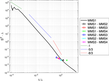
Figure 3. Second-order structure function of the magnetic field, shown as an equivalent spectrum, i.e., multiplied by the scale and plotted against the inverse scale. λ is in units of di . The black line corresponds to the single-spacecraft calculation using the Taylor hypothesis. The single points correspond to the two-point quantities for each pair of MMS spacecraft. Slopes of −1, −5/3, and −8/3 are shown for reference.
Download figure:
Standard image High-resolution imageWe also compute the second-order structure function S(2)(λ) directly from the six available two-point measurements afforded by the four MMS spacecraft. These also are plotted as six corresponding points on the equivalent spectrum in Figure 3. We note that the approximately collinear separation of the MMS spacecraft is in a very different direction, almost perpendicular to radial, compared to the sweeping of the solar wind plasma past the spacecraft in the near-radial direction that is employed in the curve obtained from the Taylor hypothesis, as shown in the diagram of Figure 1. We also take note of the separations of the MMS spacecraft, which range between 0.3 di and 2 di . These values are centered about the transition from inertial range to sub-ion scales where kinetic effects typically become important in the weakly collisional solar wind.
It is clear from Figure 3 that there is rough agreement between the two-point measurements and the single-spacecraft measurements, but in detail, there is some variation. There is also a flattening in each case, which we believe to be of different origins. We now provide a brief discussion of these physical and instrumental factors.
Two physical effects for the difference in the two types of spectra come to mind. First, intrinsic time variation would tend to make the Taylor hypothesis structure function have relatively higher values (Matthaeus et al. 2010). Second, correlation anisotropy is another major effect: the Taylor measurement is sensitive only to radial variations, but the two-spacecraft measurements are each sensitive to variations along the interspacecraft baselines, an effect noted previously for the magnetosheath (Chasapis et al. 2017). In the present case those baselines are along the string-of-pearls orbit, almost perpendicular to the radial direction. In this regard the flatter trend of the two-spacecraft measurements could be indicative of the episodic occurrence of large increments between the closely separated MMS spacecraft. These can occur when structures such as current sheets or tangential discontinuities pass between the spacecraft pairs. For the beads-on-a-string configuration this would occur when the gradients across the current sheet lie in the direction transverse to the solar wind flow. These would be detected by the spacecraft pair increments, but for the single-spacecraft (Taylor hypothesis) case, these could be spread out due to an oblique passage, or even missed entirely.
Instrumental effects can also influence the two types of spectra. In this regard the effect of noise always needs to be considered. Although, the measurements of the smaller increments estimated here are close to the noise floor in frequency, we believe based on prior studies that the frozen-in Taylor measurements are reasonably accurate up until frequencies corresponding to about 2 or 3 di , where a shallower slope is observed. For a detailed discussion of the effects of the FGM noise floor on MMS magnetic field spectra in the solar wind see Chhiber et al. (2018), especially Appendix A of that paper. The effect of noise in the two-spacecraft data points is also discussed there.
5. Turbulence Analysis
The turbulence campaign configuration permits several types of studies to be done that have not been possible previously in single data intervals. Apart from the simultaneous observations of several collinear spatial lags it is also possible to study conditional statistics relative to the direction of the magnetic field. Here we will show results relative to the local field direction (computed as the instantaneous average of the four spacecraft), with the understanding that such results in general represent a higher-order statistical quantity and are not, for example equivalent to statistics, e.g., spectra, measured relative to a well-defined mean field (Matthaeus et al. 2012). The variability of the field direction relative to the interspacecraft separation vector  during the chosen 5 hr sample provides reasonably good coverage across a wide range of angles
  . The distribution of
  is shown in the top panel of Figure 4.
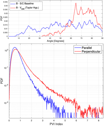
Figure 4. Top: probability distribution function (PDF) of the angle between the spacecraft separation vector and the measured magnetic field direction in blue. Also shown is the PDF of the angle between the magnetic field and the radial direction, along which the solar wind is flowing. Bottom: distribution (PDF) of the two-point partial variance of increments (PVI) conditioned on the angular ranges—parallel and perpendicular—of  . (See the text for details.) PVI is computed from increments (differences) between the MMS2 and MM3 measurements of magnetic field.
Download figure:
Standard image High-resolution imageMaking use of this broad distribution of angles we can measure anisotropy of the fluctuations relative to the magnetic field direction. For a first result of this type, we compute the PVI based on the separation between MMS2 and MMS3, which are separated by ∼200 km (∼2di
). We impose a condition on the direction θ when accumulating the  ). The parallel PDF corresponds to accumulated measurements of PVI when the angle between the spacecraft separation and the local magnetic field is between 0° and 30°. The perpendicular PVI is computed from data when the angle
  lies between 60° and 90°. It is clear that larger values are found more frequently in the perpendicular PVI. This suggests structures, such as current sheets, that are oriented such that their maximum rate of change is more in the perpendicular direction.
It should be noted that while there are fewer data points when the field is close to parallel compared to the near perpendicular case, the PVI is a normalized statistical quantity and therefore not generally impacted by the sample size, as long as the sample size is sufficiently large. This is also the case for the scale-dependent kurtosis examined in the next section. The sample size has to be large enough to accurately reflect the statistics of the turbulence, a condition that is satisfied for this interval, since it was specifically selected to have a duration much larger than the typical correlation scale of solar wind turbulence. A more detailed discussion of the relevant timescales for this interval is carried out in Bandyopadhyay et al. (2020).
Another interesting feature of the PVI distribution (not illustrated) is that the functional form of the MMS2–MMS3 PVI distribution accumulated without regard for magnetic field direction is very nearly identical to the PVI computed from the Taylor hypothesis applied to the magnetic field data from MMS1 at a time lag of 0.625 s, which corresponds to a spatial lag of about 201 km. Of course, that spatial lag is in the radial direction, while the MMS2–MMS3 PVI distribution is spatially lagged in a direction approximately perpendicular to the radial. The joint distribution of these two PVI measurements is amorphous, suggesting that they are not correlated. The magnetic field direction does not enter in either of these two computations, and from the top panel of Figure 4 one can see that angles are broadly sampled in both the MMS1-Taylor case and the MMS2–MMS3 case. A reasonable conclusion is that the signals are both pointwise anisotropic, but averaged over angles in a such a way that their overall distributions are very similar. This hints at a lack of sensitivity to the radial direction of the orientation of current sheets and other fine-scale structures, and therefore insensitivity to overall solar wind expansion.
Spectral and higher-order features as well as anisotropy can be further explored by computing second-order structures functions conditioned on local magnetic field direction, and carrying this out for spatial lags corresponding to each of the six MMS interspacecraft separations. The results of this analysis for the 5 hr campaign period are shown in the top panel of Figure 5. One sees the expected trend for higher energy levels (larger structure function S2) for large interspacecraft separation. This is of course expected based on standard spectrum results such as shown in Figure 3. The results are accumulated in nine angular channels of 10° conditioned on ranges of the angle  . This corresponds to the horizontal axis in Figure 5. We can see that the power at the smaller lag is almost independent of the angle
  of the vector lag relative to the local magnetic field. However, at progressively larger spatial lags, a prominent anisotropy emerges, with a peak in the structure function around 60°–70°. As expected from MHD and plasma theory and simulation, the gradients are stronger in the perpendicular direction than in the parallel direction.

Figure 5. Top: second-order structure function (energy) as a function of scale and angle  , for the 5 hr interval. Curves correspond to six MMS pairs, with separations 25, 57, 86, 119, 144, and 201 km. Horizontal axes correspond to bins of angles into which the structure functions are sorted for the entire interval. For the distribution of angles, see Figure 4. Bottom: two-point scale-dependent kurtosis of the magnetic field for varying angle
  , as above. Peaks are seen in both plots at 60°–70°.
Download figure:
Standard image High-resolution imageA similar conclusion is found for analysis of the angular dependence of the two-point scale-dependent kurtosis of the magnetic field, shown in the bottom panel of Figure 5. The conditioned scale-dependent kurtosis is defined as

where ℓ denotes the longitudinal direction along which the increment of the field is calculated. This corresponds to the radial direction for the single-spacecraft estimate based on the Taylor hypothesis, while for the two-point estimate it corresponds to the direction of the spacecraft formation  . A kurtosis κ = 3 indicates a Gaussian distribution that is essentially space filling, while a kurtosis larger than three indicates a non-space-filling distribution of structure consistent with fine-scale coherent structures such as vortices or current sheets. We found that the maximum value of the kurtosis decreases with decreasing spatial lag, with the largest values observed by the pair of MMS2–MMS3, which had the largest separation at 201km, or about two ion inertial scales, and the smallest values observed by the pair of MMS1–MMS4, which had the smallest separation at 29 km. Furthermore, the angular variation also shows a strong peak in kurtosis at all lags but the smallest, at around
  ≈ 60°–70°. This is essentially the same angle where the peak energy was found above.
The latter result can be visualized in a possibly more revealing way by plotting the scale-dependent kurtosis at each scale in several ways. Figure 6 shows the single-spacecraft Taylor-hypothesis-based scale-dependent kurtosis from MMS1, along with three sets of points (with errors bars for lag). These correspond to the parallel orientations with  in blue, the perpendicular orientations with
  in red, and the case of all data averaged over angle shown in black. One observes that each set of points follows trends similar to the Taylor hypothesis result. However the perpendicular results follow a trend line clearly above the Taylor result, while the parallel results lie well below the Taylor result. The results from all directions points lie between the others, and actually very close to the Taylor hypothesis analysis line.
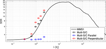
Figure 6. Scale-dependent kurtosis results from: Taylor hypothesis applied to MMS1 magnetic data (solid black line); perpendicular angles (red symbols); parallel angles (blue symbols); all angles (black symbols). The horizontal error bars show the small change in spacecraft separation during the 5 hr interval.
Download figure:
Standard image High-resolution image6. Conclusions
Well-equipped multiple-spacecraft missions flying in special formations designed to make statistical measurements of plasma moments and electromagnetic fields in space plasmas show great promise in revealing properties in space plasma turbulence at previously inaccessible level of detail (Matthaeus et al. 2020). In the early months of 2019, the reconfiguration of the four MMS spacecraft in a turbulence campaign provided such an opportunity. Here we have reported some of the first results of that campaign, making use of the variably spaced collinear formation to carry out analyses of proton- and sub-proton-scale statistics of relevance to plasma turbulence studies (Sahraoui et al. 2009; Salem et al. 2012; Alexandrova et al. 2013; Bandyopadhyay et al. 2020). Our main goals have been to compare results from the Taylor hypothesis with native two-point correlations, and to examine second-order structure functions and scale-dependent kurtosis. These analyses have been carried out here using a single long (5 hr) interval in the magnetosheath during the MMS turbulence campaign. To afford angular coverage where needed, we refer the observation direction to the local magnetic field. This procedure, though favored in some studies (Chen et al. 2011), introduces a random coordinate system, forcing a reinterpretation of standard statistical measures in terms of higher-order correlations (Matthaeus et al. 2012). Understanding these trade-offs in adopting a local measure of the preferred magnetic direction, we proceed using this approach here as it enables evaluation of scale-dependent and angle-dependent statistics with a single interval of MMS data.
The results presented here confirm a number of prior results; however, obtained here using a single interval and a unique multispacecraft configuration. The results presented on comparison of equivalent spectra to six two-point multispacecraft measurements, confirm prior results (e.g., Chhiber et al. 2018) in this new configuration. Notably, with the spacecraft in a collinear configuration, several two-point correlations have aligned baselines, removing any ambiguity that might be associated with undetected or uncontrolled anisotropy.
Additional results were obtained for second-order structure functions at six collinear spatial scales, and at the same time at a wide rage of angles relative to the measured local magnetic field direction. As typically reported previously we find stronger gradients perpendicular to the magnetic field and weaker gradients parallel to it. Finally, an analysis of the scale-dependent kurtosis found a general decrease as smaller scales approached the ion kinetic scales from above.
This is a further confirmation of the puzzling result that scale-dependent kurtosis decreases with decreasing lag in the solar wind for lags near and below the ion inertial scale. This stands in contrast to the generally observed increase of scale-dependent kurtosis with decreasing lag in the MHD inertial range.
The peak in both the variance and in the kurtosis at about 60°–70° is highly reminiscent of the results of Leamon et al. (2000), who examined best fits to physical models of the spectral break seen in solar wind spectral as the scales approach the kinetic range. They found the best fit, for the several models they experimented with, was for a parameterized set of current sheets oriented with their normals (fastest gradients) at about 75° relative to the mean field, a value very similar to the 60°–70° value found here with an entirely different method. Here we see and confirm a result that required more than 30 intervals (Leamon et al. 2000), but here with a single 5 hr burst period. Note that this result refines the concept of transverse anisotropy, but remains consistent with the standard viewpoint on quasi-2D anisotropy.
The present results in fundamental characterization of solar wind magnetic field turbulence properties remove several types of ambiguity in measurements associated with time variability, potential failure of the Taylor hypothesis, and uncontrolled variations of parameters connected with the use of multiple data sets. This approach also points the way to further multispacecraft campaigns and opportunities, as well as use of special methods that can be implemented using modern multispacecraft constellations, beginning with MMS and Cluster. Larger separations, including larger separations in linear formation, would allow probing a broader range of inertial range scales. Such more widely separated formations may be available in an MMS extended mission or in proposed missions such as HelioSwarm (Spence 2019), Debye, and others. This kind of multipoint analysis of plasma turbulence observations, free of single-spacecraft complications such as spacetime ambiguity, promises to dramatically expand our understanding of plasma turbulence as an important phenomenon in many space and astrophysical plasmas.
This research is partially supported by NASA under the MMS mission Theory and Modeling Team grants NNX14AC39G and 80NSSC19K0565, by Heliophysics Supporting Research grants NNX17AB79G and 80NSSC18K164880, and by Helio-GI grant NSSC19K0284. This research was also supported by NASA grant 80NSSC19K1469. We thank the SITL selection team, including Tai Phan, Benoit Lavraud, Sergio Toledo-Redondo, Julia Stawarz, Rick Wilder, and Olivier Le Contel for helping to select several Solar Wind intervals during the campaign. We are grateful to the MMS instrument teams, especially SDC, FPI, and FIELDS, for cooperation and collaboration in preparing the data. The data used in this analysis are Level 2 FIELDS and FPI data products, in cooperation with the instrument teams and in accordance their guidelines. All MMS data are available at https://lasp.colorado.edu/mms/sdc/. The Wind data, shifted to Earth's bow-shock nose, can be found at https://omniweb.gsfc.nasa.gov/. The authors thank the Wind team for the proton moment data set.
Appendix: Analysis of Variability of the Turbulence
The analysis presented here relied on time-averaging over the entire 5 hr interval shown in Figure 2. This implied that the observed properties of the turbulence remained stationary during this period. In order to examine the validity of this assumption we divided the 5 hr interval into five 1 hr subintervals, and examined their variability. The intervals are shown in Figure 7, with each one shaded a different color. The magnetic field and PVI Index are shown for each interval. We note that they while they are overall very similar, the first hour (shaded in red) is calmer than the rest of the interval with less sharp gradients and spikes in the PVI, which are usually associated with current sheets. Conversely, the last hour (shaded in cyan) shows the strongest activity with several very strong current sheets observed during this period. The second-order structure function and the scale-dependent kurtosis of the magnetic field are shown in Figure 8. We see that all intervals exhibit similar behavior. Still the lower level of fluctuations during the first interval is evident by the lower values of the corresponding structure function. Additionally the abundance of strong current sheets during the last hour is clearly seen on the right, where the scale-dependent kurtosis has the largest values during this interval.
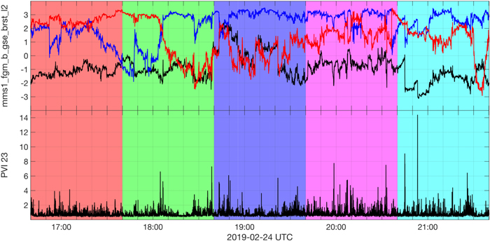
Figure 7. Magnetic field (top) and PVI Index (bottom) during the interval. The shaded colors represent each analyzed 1 hr subinterval.
Download figure:
Standard image High-resolution image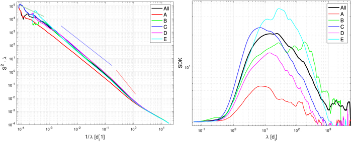
Figure 8. Second-order structure function (left) and scale-dependent kurtosis (right) of the magnetic field for each of the subintervals shown in Figure 7.
Download figure:
Standard image High-resolution image