


Abstract
There is not currently a consensus on the process responsible for producing the waiting time distribution of solar flares. This study presents an information theoretical approach to determining whether solar flare data are significantly distinguishable from a nonstationary Poisson process. A study of solar flares stronger than C1 class detected by the Geostationary Operational Environmental Satellite from 1975 to 2017 was performed. A sequence of waiting times (time elapsed between adjacent X-ray flare peaks) was constructed from the data. Surrogate waiting time sequences were produced using a time-varying Poisson firing rate from the Bayesian block procedure. Utilizing Shannon entropy, the mutual information of time-lagged waiting time distributions was computed for both the original data and the surrogates using a method of discretization by binning. When the entire period is considered, we see that when compared to carefully constructed surrogates, there is a significant elevation of mutual information on a timescale of approximately 30 hr, demonstrating that flares are confidently related to subsequent flares, contradicting the null hypothesis that flares are produced by a nonstationary Poisson process. When only 4 yr subsets of the data are considered, we see that at relatively small timescales (on the order of 10–30 hr), solar flare waiting times have a significant impact on subsequent flares. When corrected for the number of points in each considered time window, there is no correlation between the magnitude of significance and position in the solar cycle.
Export citation and abstract BibTeX RIS
1. Introduction
Solar flares are a sudden increase in the brightness of the Sun that occurs when energy stored in twisted magnetic fields in active regions is released (Toriumi & Wang 2019). The energy released in flares can be enormous, leading to immediate increases in the electron density in the ionosphere, which can interfere with radio communications and orbital decay (Bala et al. 2002; Liu et al. 2006). While the underlying evolution of the active regions is relatively slow (on the order of days to months), the duration of flares is relatively fast, ranging from minutes for weaker flares to hours for stronger flares. As such, the flares provide an "instantaneous" snapshot of the underlying dynamics of the active region. It is well known that the dynamics of systems can be well described and reconstructed by considering the set of time intervals of the system, known as waiting times (Sabatelli et al. 2002; Davidsen & Goltz 2004; Lee et al. 2005).
The distribution of waiting times has been studied intensely in solar physics (Boffetta et al. 1999; Moon et al. 2001; Wheatland & Litvinenko 2002; Moon et al. 2003; Aschwanden & McTiernan 2010; Aschwanden 2011). A key question that has been addressed is whether flares are independent events or the occurrence of one flare makes another flare more or less likely (Wheatland et al. 1998). One of the key features of the waiting time distribution is a departure from a pure exponential (Poisson) distribution that is expected for self-organized criticality (SOC) models. While SOC models predict a Poisson distribution, variable driving of SOC models results in a nonstationary Poisson distribution characterized by a power law at long waiting times (Aschwanden 2019). Several studies have suggested that the solar flare waiting time distribution could be produced by a nonstationary Poisson process where the flaring rate changes with time (Wheatland 2000b; Aschwanden & McTiernan 2010; Aschwanden 2019), leading to a power law in the tail of the distribution of waiting times  with
with  (where Δ is a waiting time) that depends on how the rate changes in time. In principle, such a distribution could be produced either through a sequence of time periods having different flaring rates or through multiple Poisson processes having different flaring rates acting simultaneously. More recent studies, such as Telloni et al. (2014) and Li et al. (2018), suggest that the waiting time distribution of weaker flares may be closer to a Weibull distribution, which describes a distribution having a characteristic size with an additional parameter that takes into account the spread of sizes.
To date, most studies have focused on the probability distribution of solar flare waiting times  , where
  is a sequence of waiting times drawn from the waiting time distribution. These studies have examined how well this distribution can be fit with different processes, and the closeness of fit is typically determined by a test such as the Kolmogorov–Smirnov test, which compares the cumulative distribution function with a test distribution based on a null hypothesis. However, because many processes could map to the same probability distribution, there may be some ambiguity in drawing conclusions about the random process responsible for the sequence of waiting times based only on the probability distribution function. While a comparison of waiting time distributions with distributions resulting from various random processes may be valuable for assessing the "closeness" of distributions, it does not take advantage of the additional information provided by the ordering of the flare sequence.
If the ultimate objective is to determine whether there is memory in the sequence, as some studies do (Li et al. 2018), it seems particularly useful to examine the joint probability,  , between the waiting time of a flare event and another flare event having a "look-ahead" of m. For example, if m = 1,
  describes the joint probability between the waiting times of successive flares. In particular, if we wanted to establish whether or not subsequent waiting times are independent, then we could examine whether

The comparison described by Equation (1) can be established using the mutual information (MI), defined as

where

are the Shannon entropies of the random variables  and
and  , and
, and

is the joint entropy. The mutual information is particularly useful to establish nonlinear relationships between two random variables. It is apparent that when X and Y are independent,  , providing a method to test whether the sequence is statistically independent or dependent.
As a simple example, consider the distribution obtained by a sequence of coin flips. If the coin flips were random (and if we have a sufficiently large sequence), we would expect that half of the coin flips would be heads and half would be tails. On the other hand, if we use a double-headed and double-tailed coin for every other flip, we would also find that half of the flips are heads and half are tails. While the distributions are identical, the underlying processes are completely different. On the other hand, using the mutual information, it is relatively easy to distinguish between the two processes. For example, if we consider X to be a coin flip and Y to be the following coin flip, then  for an unbiased coin, while for the biased coins,
  or 1 bit of information (using base 2), consistent with the fact that the result of the next coin flip is completely determined from the prior flip.
Following this line of reasoning, if we want to determine whether flare events are statistically independent, we could consider the mutual information of the time-lagged distribution,  . Here mutual information provides a measure of whether subsequent flares are dependent or independent, and we can also determine how far ahead this dependence lasts, effectively providing an information horizon for the memory of flares. This discriminating statistic can also be computed using subsets of the data within various time windows to determine how the underlying dynamics responsible for the memory changes over time. Time-lagged mutual information has been applied to a number of problems (Johnson & Wing 2005, 2014, 2018; March et al. 2005; De Michelis et al. 2011; Materassi et al. 2011, 2014; Balasis et al. 2013; Wing et al. 2016; De Michelis et al. 2017; Johnson et al. 2018; Wing et al. 2018; Wing & Johnson 2019; Wing et al. 2020).
In the following sections, we first present the flare data set in Section 2. Under the assumption of a null hypothesis, where the data result from a nonstationary Poisson process, we provide a method for transforming the data into a stationary Poisson series in Section 3 which allows for creation of surrogates also satisfying the null hypothesis, presented in Section 5. Mutual information, the metric used to discriminate between the original data and the surrogates, is presented in Section 4. Finally, the results of the analysis are presented in Section 6 and inconsistencies between the findings and the null hypothesis are discussed in Section 7, supporting the notion that there exists memory within the flaring system.
2. Data
The solar flare data for this study were obtained from the Geostationary Operational Environmental Satellite catalog of flares from 1975 to 2017, available from https://www.ngdc.noaa.gov/stp/solar/solarflares.html. In keeping with previous studies, such as those by Moon et al. (2001) and Wheatland & Litvinenko (2002), we consider only flares with a peak flux greater than  . This threshold is chosen to reflect the difficulty of detecting flares below class C1 (
 ), as much of the time, these low-energy events lie below the background flux (Hudson 1991). Event times were taken to be the time of maximum flux during bursts that fit the above criteria.
From this sequence of nearly 72,000 flaring event times,  , we construct a sequence of waiting times,
  , where
  . This time sequence, shown in Figure 1, contains more information about the dynamics of the system than just the waiting time distribution. Most apparent in Figure 1 is the clear periodicity of the waiting times, which is unsurprising given the solar flare activity's dependence upon position in the solar cycle (Hathaway 2015).
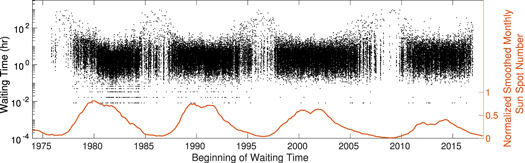
Figure 1. Waiting times (mean of 4.83 hr) are scattered at the time corresponding to the first flare of each pair. The curve near the bottom of the figure is the SSN obtained from the SILSO World Data Center (1974) and is used throughout this study.
Download figure:
Standard image High-resolution imageFor our analysis, waiting times greater than 1000 hr are expunged from the series to adjust for waiting times that are the result of gaps in the data due to possible instrument maintenance or bad data flags resulting in missed events. The waiting time distribution of the data with the cutoff performed is shown in Figure 2. Note that while our choice of 1000 hr is somewhat arbitrary, the results are insensitive to this cutoff. Statistics are extremely poor this deep into the tail of the waiting time distribution. Even if these waiting times are real, they do not significantly affect the result, as simply deleting these long waiting times, which account for less than 0.5% of the data, changes the mean waiting time and significance of the result by less than 5%. One should also note that there is also a discrepancy at small waiting times. Currently, there is no consensus as to whether this is physical and the result of some other process (such as a Weibull process) or whether it is the result of observational error or failure to separate near-simultaneous flares (Wheatland 2005; Li et al. 2018).

Figure 2. Waiting time distribution for the entire period (1975–2017) and a stationary Poisson distribution with the mean firing rate, 0.207 flares hr–1. Error bars for the data are given by  .
.
Download figure:
Standard image High-resolution image3. Creating Stationary Poisson Series
Ultimately, we want to determine whether the sequence of solar flare waiting times is consistent with the null hypothesis of a nonstationary Poisson process. As such, we assume that the null hypothesis is true and then show inconsistency with this assumption. If the null hypothesis were true, then the solar flare waiting time distribution should be consistent with a nonstationary Poisson process (essentially a Poisson process with a variable rate). To construct surrogate data for comparison, it is necessary to determine how the rate changes with time. Different methods can be used to determine how the rate varies in time, such as averaging the number of events over a sliding time window (Moon et al. 2001) or using a Bayesian block (BB) procedure (Wheatland 2000a; Wheatland & Litvinenko 2002), and both methods result in waiting times consistent with the solar flare waiting time distribution. The BB procedure is a nonparametric method that takes a sequence of event times and determines a decomposition into intervals of time when the observed event occurrence is consistent with a (constant rate) Poisson process (Scargle et al. 2013). These intervals are characterized by a duration and a rate and are called BBs. Given a set of data and a single parameter determining the prior (an initial guess on the number of blocks), this algorithm is guaranteed to find the global optimum piecewise constant firing rates that describe the data within observational errors. The resulting BB decomposition, shown in Figure 3, was found to be quite insensitive to the only free parameter. An earlier version of this tool was used in a similar study by Wheatland & Litvinenko (2002). Notably, the old version was greedy (suboptimal) and replaced by an efficient and exact algorithm (Scargle et al. 2013).
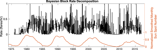
Figure 3. The BB decomposition of the flare firing rate. The mean block length is 24 days. The variance of the rate corresponding to the solar cycle is easily visible.
Download figure:
Standard image High-resolution imageIn Figure 4, we show the waiting time distribution that results from the BB decomposition shown in Figure 3. For comparison, we also show the original data in blue. The waiting time distribution of the BB models the data very well, consistent with previous analyses of solar flare waiting times as a nonstationary Poisson process (Wheatland 2000a; Moon et al. 2002). The inset figure also shows the same data on a log–log plot, which emphasizes that the BB decomposition captures the power-law behavior of the data at long waiting times. The power law of the tail of the distribution is asymptotic to −2.5 and within the range that has been reported (between −2 and −3; Wheatland 2000b; Aschwanden & McTiernan 2010).
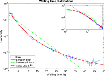
Figure 4. Same as Figure 2 but also showing the waiting time distributions from the weighted piecewise Poisson model with rates from BBs. The inset figure is a log–log plot of the same distribution and also shows that the distribution is asymptotic to a power law  at long waiting times.
Download figure:
Standard image High-resolution imageAssuming the solar flare data result from a nonstationary Poisson process (consistent with the null hypothesis), its BB decomposition will provide an ensemble of Poisson processes, where each BB is a realization of a stationary Poisson process characterized by its mean firing rate. If we scale each waiting time by the rate of the block to which it belongs, then the result is an ensemble of Poisson processes, all with unit rate, as confirmed in Figure 5. As the process is assumed stationary, the ensemble average over the blocks should be equivalent to an average over the sequence. It is conceivable that in this scaling process, there are "edge effects" due to waiting times represented by flares in different blocks. However, the average number of waiting times per block is approximately 100 (blocks are well represented), and adjacent blocks have similar rates, so it is expected that edge effects are negligible.
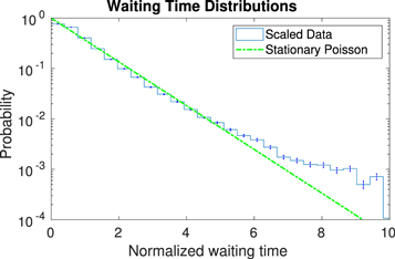
Figure 5. Waiting time distributions of the scaled data and a unit Poisson. The mean scaled waiting time is 1.01. Deviation occurs deep into the tail, where observational statistics are poor. Only approximately 0.5% of scaled waiting times are above 6, where the deviation occurs.
Download figure:
Standard image High-resolution imageThis sequence is suitable for testing the null hypothesis that the original sequence is generated by a nonstationary Poisson process. With this null hypothesis, the scaled sequence should not be different from a sequence generated by a stationary Poisson process. Mutual information provides a discriminating statistic to compare the scaled sequence with surrogate sequences satisfying the null hypothesis, which have a theoretical mutual information of zero. By scaling the data in the above way, we have removed information due to fluctuations in the firing rate on large timescales (on the order of 24 days, the average block length), such as the solar cycle or variations in the number of active regions. This block length is consistent with previous studies that found block lengths approximately equal to the average active region crossing time to be appropriate for a nonstationary Poisson model of these data (Wheatland 2000a; Moon et al. 2002). Without this step, one can imagine that there would exist clusterings in the time-lagged distribution that would be centered around different time-local firing rates, which may contribute to a nonzero MI.
It should be noted in this approach that we map the observed waiting time sequence using the BB block decomposition (consistent with the null hypothesis) so that it can be compared with surrogate data constructed from an equivalent stationary Poisson process. Alternatively, we could use the BB decomposition to construct surrogates consistent with a nonstationary Poisson process that can be compared directly with the waiting time sequence. Inconsistency using either approach is sufficient to falsify the null hypothesis. We found that the first approach provides a cleaner result because the mutual information should vanish if the null hypothesis is satisfied.
4. Mutual Information Calculation
The primary challenge to computing the mutual information involves inherent uncertainties in the data and sample-size estimator bias. Uncertainties in the waiting times involve instrument biases, data gaps, and biases introduced by the arbitrary definition of a flare, including the threshold, onset time, and separation of simultaneous flares. Sample-size bias manifests itself through an uncertainty in determining the probability distribution function. In this study, mutual information is calculated using a method involving a discretization or quantization of the data by bin assignment. Quantization of data inherently leads to quantization errors in the estimate of mutual information. Mutual information is of little value if the number of quantized levels is either too small (all data are contained in one bin) or too large (bins are sparsely populated and generally only have one observation per bin). It should also be noted that the mutual information generally increases logarithmically as the bin size decreases until it saturates as the number of quantization levels approaches the (size of the data set)1/n, where n is the number of dimensions of the probability distribution. These issues make it challenging to identify a regime where the number of quantization levels is small enough so that errors are not introduced by the size of the data set but large enough so that it is possible to distinguish the difference in mutual information. As an example, random data should have mutual information that tends to zero, but as long as there is only a limited amount of data, this baseline will not generally be met. For this reason, we compare our results with surrogate data (see the following section detailing surrogate construction) that are constructed based on a null hypothesis and share the same shortcomings as the original data in terms of quantization, so that any features that result through the quantization process can be eliminated.
Though this binning method is efficient, it is not perfectly ideal, as the bin size is a free parameter. As discussed above, choosing a bin size at either extreme, including all points in one bin or only one point in each bin, will yield well-defined but practically useless quantities. We are interested in differentiating the data from a collection of surrogates. Therefore, in Figure 6, we show that there exists a region of bin sizes where the significance of discrimination between the data and the surrogates is stable. The bin size roughly at the center and maximum of this elevated significance was chosen for the entirety of this analysis. For the results presented in this paper, we use a discrete bin size consistent with this benchmarking analysis.
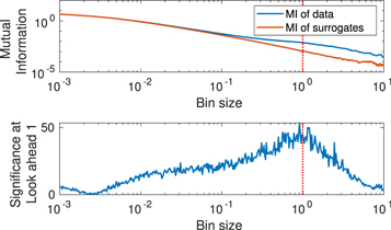
Figure 6. Top: comparison of the mutual information of the entire original data set and the surrogates for a wide range of bin sizes at a look-ahead of 1. Note that both curves follow the same trend toward the extremes. Bottom: discriminating significance plotted vs. bin size. Note the broad range of bin sizes where significance is elevated. The bin size used throughout this study is plotted with the vertical dashed line.
Download figure:
Standard image High-resolution image5. Surrogates
Our goal is to determine whether flare events are statistically independent. As previously mentioned, a stationary Poisson process has zero MI. However, any calculation of mutual information from some sampling of such a distribution could be expected to be nonzero due to tool error or as a consequence of finite data. In order to interpret mutual information results from the data, we construct an ensemble of surrogate data sets so that we can calculate significance, α, given by

where  is the mutual information of the data;
  is the mean mutual information obtained by averaging the mutual information of each surrogate data set,
  , over the number, NS, of surrogates,

and  is the standard deviation of those surrogate mutual information calculations,

This standard metric for discrimination is used throughout this study.
In this study, surrogates are constructed by randomly permuting (shuffling) the list of waiting times blockwise. That is, only waiting times associated with the same block are exchanged, rather than shuffling the entire list. This method is utilized in the endeavor to prevent exchange between time periods with very different firing rates, as these periods may be governed by dissimilar physical processes. This approach would be more likely to preserve some of the MI due to these relatively time-local effects than would simply shuffling the entire series. Further, this takes a step in the direction of isolating the error the BB decomposition may make in identifying appropriate blocks. Creating surrogates by blockwise shuffling presents a strong conclusion should the MI of the data and surrogates differ, as the waiting time distributions are naturally identical and time-local effects are preserved on the order of the average block length, 24 days. Throughout this study, 50 surrogates were created and then treated the same as the original data. It should be noted that the autocorrelation of the flare events discussed in the following section does not differ significantly from that of the surrogates.
6. Results
In Figure 7, we see that when the time-lagged distributions for the entire period from 1974 to 2018 are considered, there exists a highly elevated significance that extends to around a look-ahead of 6. As the average waiting time for the entire period is 4.83 hr, this elevated memory can be considered to persist, on average, for about 30 hr. Considering the entire period provides the best statistics because it allows for a much larger data set, resulting in an increased capability to discriminate between the surrogates and the data. However, this approach does not show in any way how this information metric may change over large timescales, for instance with fluctuations in the solar cycle. To produce Figure 8, a 4 yr sliding window was stepped at 2 month increments, with the same process as for Figure 7 performed at each step for the scaled waiting times corresponding to the window. The analysis at each time step naturally has a different number of waiting times, but the scaled data are all members of the now-stationary distribution.

Figure 7. Significance, as defined in Equation (5) (solid blue line), vs. look-ahead for the entire period (1974–2018). The dashed red line is shown at a significance of 3, illustrating that significant information persists to a look-ahead of 6.
Download figure:
Standard image High-resolution image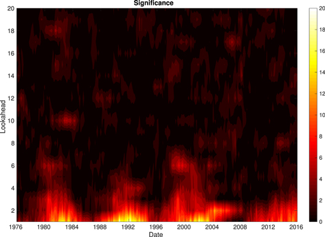
Figure 8. Contour plot showing significance vs. look-ahead vs. time.
Download figure:
Standard image High-resolution imageFigure 8 clearly shows that significance is elevated to some appreciable degree throughout the entire 44 yr period. Note that there does appear to be a dependence on the magnitude of this significance with position in the solar cycle, with lower significance occurring at solar minimum. This is believed to be due to different amounts of data in each 4 yr period and is further explored later in this section.
Figures 9 and 10 show slices of the contour plot, Figure 8, taken at times during solar maximum and minimum, respectively. However, instead of being plotted versus look-ahead, here we have multiplied the x-axis by the mean waiting time in each 4 yr period. Now the significance of these periods can be compared in the time domain, and we see that they all follow similar trends, albeit with different granularity. One useful way of characterizing the curves found in Figures 9 and 10 is by their intersection with a significance of 3. This characterization can be thought of as an information horizon, or how long it takes until we can no longer confidently differentiate the data in the window from a nonstationary Poisson process. This horizon has been plotted in Figure 11 for each window, along with the monthly smoothed sunspot number (SSN). There is no clear correlation between the two, which suggests that whatever process is responsible for the elevated mutual information does not significantly depend on the solar cycle.
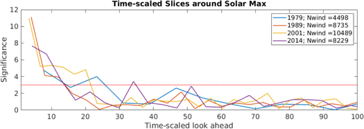
Figure 9. In this figure, slices of Figure 8 are taken at a number of times near solar maximum, and look-ahead is multiplied by the average waiting time in hours within each window, scaling the x-axis for each curve individually. This yields a meaningful time measure of how many hours memory confidently persists.
Download figure:
Standard image High-resolution image
Figure 10. To produce this figure, the same procedure as for Figure 9 was performed for windows centered in solar minimum. Note that since the mean waiting time is much larger for these periods, we have a much coarser time granulation.
Download figure:
Standard image High-resolution image
Figure 11. Amount of time each window shown in Figure 8 takes to drop below a significance of 3 or the information horizon is plotted above the monthly SSN. There is no clear correlation. Note that some obvious irregularities can be seen in the top curve at the beginning of the period, as well as during 2006–2009. These are attributed to poor statistics due to poor observations and a very quiet solar minimum, respectively. Refer to Figure 1 for visual evidence.
Download figure:
Standard image High-resolution imageFigure 12 shows the maximum significance for each 4 yr window. As discussed above, we see what appears to be a rather smooth dependence upon position in the solar cycle, with lower significance occurring at solar minimum. However, another important value also fluctuates in a similar manner: the number of points in each window. This fact is unsurprising, as there is a direct relationship between the local firing rate and the flares' time density. Figure 13 shows that, for a sample period of 2000–2004, there is a roughly linear relationship between the number of points and the magnitude of the significance. This dependence of significance on the number of data points was found to be true throughout the entire period. Therefore, we can scale the significance for each window by the number of points to remove this dependency. The normalized and scaled maximum significance is shown in Figure 14. What is now seen is a relatively constant value with no clear periodicity related to the solar cycle.

Figure 12. Maximum significance and number of waiting times for each window are both plotted. There appears to be a strong correlation between the two.
Download figure:
Standard image High-resolution image
Figure 13. Linear relationship between number of data points and significance at look-ahead 1 for a sample period, 2000–2004.
Download figure:
Standard image High-resolution image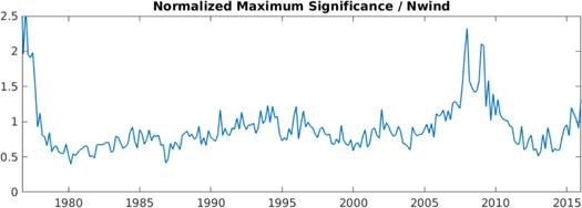
Figure 14. Here the maximum significance in Figure 12 has been normalized and scaled by the number of data points in each window. We now see that the maximum significance is nearly constant when the number of points in the window is taken into account. The elevated values seen at the beginning of the period, as well as during 2005–2010, are likely the result of the same inadequate statistics discussed in Figure 11.
Download figure:
Standard image High-resolution image
7. Discussion and Conclusions
This paper has presented an information theoretical approach to take advantage of the additional information encoded in the ordering of a time sequence beyond just its distribution. When this method is applied to solar flares, results show the following.
- 1.When the entire 44 yr period is considered, we see that when compared to carefully constructed surrogates, there is an elevation of mutual information significant to 3 standard deviations that persists to a look-ahead of 6, showing that flares are confidently related to subsequent flares on a timescale of approximately 30 hr.
- 2.
- 3.When corrected for the number of points in each considered time window, there is no correlation between the magnitude of significance and position in the solar cycle.
Consequently, we have shown that modeling flaring rates as a nonstationary Poisson process on these small timescales is insufficient to fully capture the impact of some unknown physical dynamics of the system. Regardless of how well it may capture the waiting time distribution for the entire period, there exists short-term memory within the waiting time sequence that cannot be reproduced by modeling these data as a nonstationary Poisson process. However, using the method presented in this paper at larger timescales (on the order of days to weeks), the data are indistinguishable from a nonstationary Poisson process. This result is consistent with current avalanche models, which treat the system as a Poisson process, as the waiting time distribution would suggest. Though the exact mechanisms responsible for this small timescale memory are unknown, some possible candidates are turbulence models (Boffetta et al. 1999) that show bursty or intermittent behavior, sympathetic flares, or homologous flares (Moon et al. 2002). Consolini & de Michelis (2002) introduced the idea that some waiting time distributions may be described by noise-induced topological transitions, where the transitions may involve local coupling of magnetic and plasma structures. This framework may be useful for understanding the dependence of flare waiting times at smaller timescales, where local coupling may be important (e.g., sympathetic flares).
7.1. Future Work
The method presented in this paper has far-reaching applications, as it can be used to investigate any time series data set, so long as there exist sufficient observational statistics and an appropriate surrogate. Below are several closely related areas that we have considered exploring using mutual information.
- 1.Memory between flare amplitudes and waiting times. This relation has been explored to some extent in previous studies, such as Wheatland (2000a).
- 2.Memory between flare locations. This would probe whether there exists a causal relationship between flares originating from within the same active region, or perhaps from linked active regions.
- 3.Development of a rigorous method to filter out periodicities within the data in an endeavor to remove information contributions from periodic flare systems.
- 4.Comparison of the information flow of flares and turbulence models (e.g., Boffetta et al. 1999).
- 5.Exploration of modeling flares as short-term memory stochastic processes.
Work at Andrews University is supported by NASA grants NNX15AJ01G, NNH15AB17I, NNX16AQ87G, 80NSSC19K0270, 80NSSC19K0843, 80NSSC18K0835, 80NSSC20K0355, NNX17AI50G, NNX17AI47G, 80HQTR18T0066, 80NSSC20K0704; NSF grants AGS1832207 and AGS1602855; and Andrews University Faculty Research Grant 201119.