


Abstract
The interaction of the solar wind (SW) with the partially ionized interstellar medium forms the heliosphere. As the supersonic SW flows away from the Sun and incorporates pickup ions (PUIs), they are slowed, compressed, and heated at a termination shock, creating an energetic ion population in the inner heliosheath. The neutralization of PUIs in the heliosheath creates energetic neutral atoms (ENAs) at ∼keV energies that travel ballistically and can be observed at 1 au by the Interstellar Boundary Explorer (IBEX). IBEX uses single-pixel cameras to map ENAs from the heliosphere. In this study, we analyze IBEX observations of >1 keV ENAs from the heliotail during 2009–2017. The ENA spectral index maximizes near the ecliptic plane and decreases at higher latitudes, reflecting the latitudinal structure of the SW. We show that the angular spread of this structure can be used to derive the distance at which the observed ENAs originate, i.e., their cooling length. Using Ulysses observations of the SW we determine that the distance from the Sun to the source of ∼1–6 keV ENAs in the heliotail is ≥289 ± 35 au in 2009–2013 and ≥489 ± 56 au in 2014–2017, using the distance to the termination shock in the downwind direction as 160 au based on the analysis of McComas et al. The increase in ENA source distance over time suggests that IBEX is observing a fast/hotter plasma parcel propagating down the heliotail before being replaced by slow/cooler plasma as the solar cycle evolves.
Export citation and abstract BibTeX RIS
1. Introduction
The heliosphere surrounding our Sun is formed by the interaction between the supersonic solar wind (SW) plasma and the partially ionized interstellar gas in the very local interstellar medium (VLISM). The solar and interstellar plasmas are separated at a tangential discontinuity called the heliopause. Interstellar neutral atoms travel into the heliosphere and some experience ionization by photoionization, electron impact, or charge-exchange with SW ions, forming pickup ions (PUIs). These PUIs are carried outwards with the SW as a nonequilibrated, nonthermal population. At approximately ∼100 au from the Sun the SW and PUIs are slowed, compressed, and heated at a termination shock (TS). PUIs are preferentially heated (e.g., Zank et al. 1996; Kumar et al. 2018; Zirnstein et al. 2018c and references therein) and form an energy-dominating population in the inner heliosheath (IHS). Subsequent charge-exchange between PUIs in the IHS and interstellar neutral atoms creates energetic neutral atoms (ENAs) with ∼keV energies that can ballistically travel toward Earth and be detected.
The Interstellar Boundary Explorer (IBEX; McComas et al. 2009a) is an Earth-orbiting spacecraft with a Sun-pointed rotation axis that utilizes two single-pixel cameras to detect interstellar neutral atoms flowing into the heliosphere (e.g., McComas et al. 2009b; Möbius et al. 2009; Bzowski et al. 2019 and references therein) and ENAs produced by charge-exchange in the outer heliosphere (e.g., McComas et al. 2009b, 2017, 2018; Schwadron et al. 2018 and references therein). IBEX-Hi creates all-sky maps of ENAs as a function of energy (∼0.5–6 keV) and time, providing extremely useful information on the properties of the time-varying SW–VLISM interaction (e.g., McComas et al. 2017) and the boundary distances of the heliosphere (e.g., Zirnstein et al. 2018a; Reisenfeld et al. 2019 and references therein).
IBEX observed two distinct sources of ENAs from the SW–VLISM interaction—the "ribbon" of enhanced ENA fluxes (McComas et al. 2009b) forming a narrow band across much of the sky, and the "globally distributed flux" (GDF), a more diffuse source of ENA fluxes from the entire sky (e.g., McComas et al. 2009b; Schwadron et al. 2014). The ribbon is most likely formed from secondary ENAs originating outside the heliopause in directions approximately perpendicular to the local interstellar magnetic field (see Heerikhuisen et al. 2010; McComas et al. 2014, 2017; Zirnstein et al. 2019 and references therein). The GDF largely originates from the IHS, where suprathermal protons, mostly PUIs, experience charge-exchange with interstellar neutrals and create ENAs.
Depending on the direction in the sky, the line-of-sight (LOS) path length of the ENA-generating source region, and the source plasma properties, the GDF exhibits both enhancements (nose and tail; Schwadron et al. 2014) and depletions (port and starboard lobes; McComas et al. 2013). Comparisons between simulations and IBEX observations show that the GDF from the heliotail is slightly enhanced due to the heliotail's extended length (e.g., Heerikhuisen et al. 2014), but not too enhanced due to the extinction of energetic protons by charge exchange, thus limiting the distance over which we can observe ENAs (e.g., Schwadron et al. 2014; Zirnstein et al. 2017b). Thus, the source distance of ENAs from the heliotail is within a few hundred astronomical units of the TS (e.g., Schwadron et al. 2014; Zirnstein et al. 2016a, 2017b).
In addition, the latitudinal structure of the SW, specifically the fast SW emitted from the polar coronal holes (PCHs), adds complexity to ENA emissions from the heliotail, producing northward and southward ENA tail lobes above and below the ecliptic plane at high ENA energies. The latitudinal position of these north and south lobes is consistent with the fast SW plasma propagating down the heliotail (Zirnstein et al. 2017b). The latitudinal SW structure is also visible in ENA spectral index with low spectral index (≲2) at high latitudes and high spectral index (≳2) at low latitudes (Zirnstein et al. 2017a). The coupling between the latitudinal SW structure, the latitudinal ENA spectral structure, and the distance to the ENA source is the focus of this study.
2. Observations
We analyze IBEX ENA observations taken from 2009–2017 (McComas et al. 2017, 2018) from the highest three energy passbands centered on 1.74, 2.73, and 4.29 keV. Specifically, we utilize IBEX data collected on the ram side of the spacecraft motion but corrected for the Compton–Getting effect to transform the data to the solar inertial frame. The data are also corrected for ENA losses from 1–100 au (i.e., survival probability corrected; McComas et al. 2017).
Since the ribbon is most likely produced by the secondary ENA mechanism from outside the heliopause (e.g., Heerikhuisen et al. 2010; McComas et al. 2017), we exclude pixels near the ribbon direction. We remove pixels within 20° of a circle projected onto the sky with angular radius 74 81 centered on ecliptic J2000 (21833, 4038), i.e., the mean radius and center of the ribbon (Dayeh et al. 2019), thus "masking out" most of the ribbon. Note that we do not use ribbon-separated data produced by Schwadron et al. (2014, 2018) due to the potential addition of uncertainties in the ribbon removal process.
We choose to analyze IBEX data at the three highest energies (1.74, 2.73, and 4.29 keV) since the north/south ENA tail lobes are most prominent at these energies, and the high energy.
ENA spectral index reflects the latitudinal structure of the SW propagating down the heliotail (Zirnstein et al. 2017b). The ENA spectral index, γ, is calculated over energies 1.74–4.29 keV by performing a chi-squared minimization of a linear function fit in log–log space to the data with their statistical uncertainties taken into account. We also include an estimate of the calibration uncertainty of IBEX-Hi (20% of the flux) used in previous studies (e.g., Fuselier et al. 2012, 2014). A sample of the ENA fluxes and their spectral index maps are shown in Figure 1.
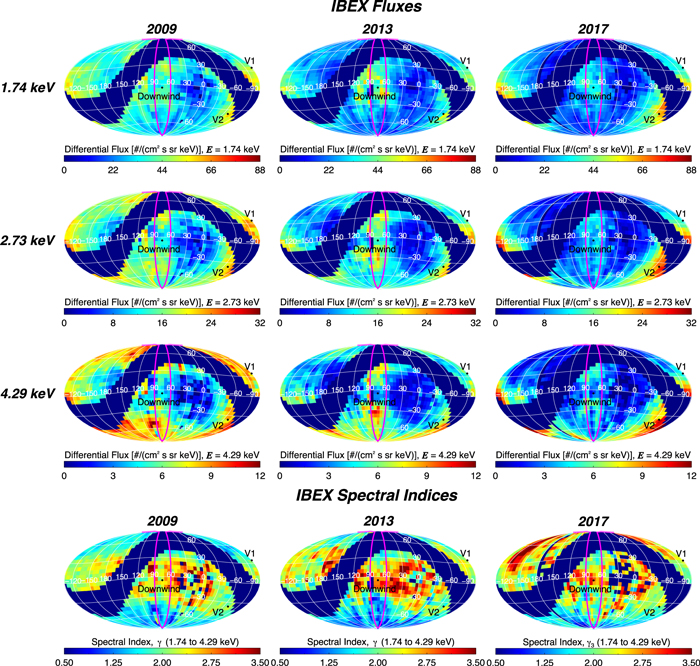
Figure 1. Sky maps of IBEX ENA fluxes and spectral indices centered on the downwind VLISM direction at energies 1.74, 2.73, and 4.29 keV from 2009, 2013, and 2017. For this study, we analyze spectral indices in the longitude range within the magenta curves, i.e., ±15° from the nearest pixel to the downwind VLISM longitude.
Download figure:
Standard image High-resolution imageNext, we reduce the data by performing a statistically weighted average in longitude within ±15° of the downwind direction (magenta curves in Figure 1). The uncertainties of the weighted averages are calculated by summing in quadrature the propagated uncertainty of the mean and the statistical uncertainty of the variation about the mean (see Appendix C in Zirnstein et al. 2016b). The reduced data are shown in Figure 2 as a function of latitude and time. A low latitude band of large (≳2) spectral index is easily visible near the solar equatorial plane, which at this longitude is nearly the same as the ecliptic plane. This band reflects the slow SW propagating through the heliotail.

Figure 2. ENA spectral index γ in the tail region of the heliosphere for energies 1.74–4.29 keV. Note that the white pixels are missing data either after removing the ribbon or unprocessed due to insufficient statistics. We also show the latitude of the solar equatorial plane as a dashed line and the north/south polar regions.
Download figure:
Standard image High-resolution image3. Analysis and Results
3.1. Simplified Structure of the SW in the Heliotail
In this study we solve for the distance to the ENA source, specifically, that in the fast SW propagating through the heliotail. Our method relies on IBEX observations of high energy ENAs from both the slow and fast SW in the IHS, as we describe below. The distance to the ENA source also depends on the latitudinal structure of the SW. Figure 3 illustrates the simplified SW structure in a meridional cut through the heliosphere. At solar minimum the fast SW is emitted from PCHs centered near the poles and extending down to midlatitudes (McComas et al. 1998; Figure 3(a)). As the SW flows past the TS, it is carried down the heliotail (Figure 3(b)).
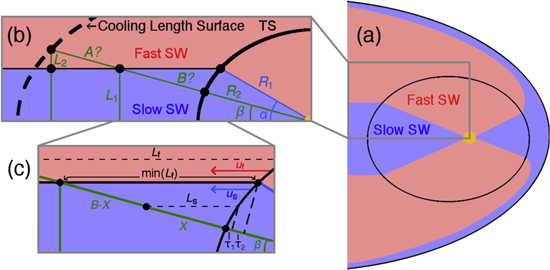
Figure 3. (a) Simplified illustration of the fast (red) and slow (blue) SW propagating through the heliosphere near solar minimum. (b) Illustration of the geometric relations between the distances from the Sun to the TS (R1, R2), the boundary between the fast and slow SW propagating through the IHS (intersecting A and B), and the unknown cooling length of PUIs (black dashed curve, A + B). Note the illustrations are not necessarily to scale. (c) Magnification of panel (b) showing the relation between the average streamline distance in the slow SW (Ls) flowing at speed us and the average streamline distance in the fast SW (Lf) flowing at speed uf. The minimum possible distance of Lf is also shown.
Download figure:
Standard image High-resolution imageIn Figure 3(b) we show a simplified geometry of the fast and slow SW as it propagates down the heliotail, assuming that the SW flow trajectory is directed downwind immediately after crossing the TS. We discuss the implications of this assumption in Section 4. The system of equations for this geometry is
Angle α defines the elevation angle from the equatorial plane of the fast–slow SW boundary emitted from the Sun during solar minimum. Angle β defines the elevation angle at which IBEX observes the transition from low to high energy ENAs emitted from the heliotail. We aim to solve for the sum of distances A + B, where A is the LOS path length in the fast SW (up to the cooling length surface), and B is the LOS path length in the slow SW.
3.2. Ulysses Observations of the SW—Angle α
First, we determine angle α from Ulysses SWOOPS observations of the SW. IBEX began taking measurements in 2009, near the end of solar cycle 23. Considering that it takes at least 2 yr for the delay between measurements of the SW and ENAs from the heliosphere (e.g., McComas et al. 2017, 2018; Zirnstein et al. 2017a; Reisenfeld et al. 2019), the timing of Ulysses' third, fast polar scan when it was ∼1.4–2.4 au from the Sun approximately corresponds to IBEX observations from 2009 and later. According to observations of the north and south PCH areas (Karna et al. 2014), the PCHs extended to their minimum latitudes around the time of Ulysses observations in ∼2007. Therefore, Ulysses observations during its third polar scan are a reasonable measurement of the minimum latitude that the large-scale, PCH fast SW was emitted from the Sun.
Figure 4 shows SW speed as a function of latitude for Ulysses' third polar scan in 2007. We determine angle α by finding the highest latitudes at which Ulysses crosses into the slow SW of the streamer belt—these crossings are seen as abrupt changes in SW speed. Starting from the poles, we compute a running standard deviation in SW speed using the three nearest bins in latitude and find when the deviation first increases above 50 km s−1. This latitude is found in both the northern and southern hemispheres, yielding the angular width of the slow SW (vertical dashed blue lines). By halving the angular width of the slow SW from Ulysses observations, we find the elevation, or half, angle α = 368 ± 044. The uncertainty of α is calculated as the square root sum of the squares of the uncertainties of each latitude found by the running standard deviation. Note that α is the minimum latitude that the fast SW is emitted from the PCHs in the IBEX epoch, and thus does not change over the times we observe.
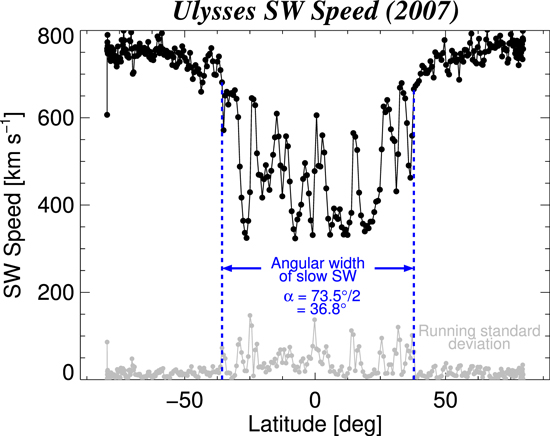
Figure 4. SW speed as a function of latitude from Ulysses SWOOPS data in ∼2007 (black). Angle α is calculated as half the angular width of the slow SW (green). The running standard deviation of a three-data point window is also shown in gray.
Download figure:
Standard image High-resolution imageWe note that there are potential systematic uncertainties in α. Specifically, the latitude at which Ulysses crosses into the slow SW streamer belt changes as a function of solar longitude as the Sun rotates with respect to Ulysses position. This is visible in Figure 4. However, we choose angle α at the highest latitude that Ulysses crossed the boundary, since we expect fast–slow SW stream interactions within the streamer belt to wear down the SW structure at large distances from the Sun and thus decrease the SW speed at low- to midlatitudes. The abrupt changes in SW speed observed by Ulysses at low- to midlatitudes is likely from corotating interaction regions (CIRs; e.g., Borovikov et al. 2012). Borovikov et al. (2012) demonstrated that as CIRs wear down with distance from the Sun, the low latitude slow SW may extend to even higher latitudes. We note that this behavior, if true, would imply our value for α would be underestimated. However, as explained later in Section 3.4, we provide a minimum distance to the ENA source in the heliotail, and an underestimation of α also implies an underestimation of the ENA source distance, consistent with our results.
To check the validity of our value for α, we also analyze SW speeds reconstructed from interplanetary scintillation observations of the SW (Tokumaru et al. 2010, 2012) following the methodology of Sokół et al. (2013, 2020). We calculate the average SW latitudinal structure from 2006.5 to 2009.5, which overlaps Ulysses observations and the minimum of solar cycle 23. We find that the latitude at which the interplanetary scintillations-derived SW speed equals a value typically used to identify the fast SW boundary (650 km s−1) is also 368. This reinforces the results derived from Ulysses observations.
3.3. IBEX Observations of ENAs—Angle β
Next, we define β as the elevation angle where the ENA spectral index is balanced by ENAs from the slow and fast SW in the IHS (ENAs produced along distances B and A, respectively). To first order this implies that the LOS-integrated fluxes produced along A are equal to those produced along B, i.e., A = B (note, however, there is a small correction to this, discussed below). One might assume this means the ENA spectral index at angle β is exactly halfway between that from the slow versus fast SW. While this is a reasonable approximation, in general, this is not true if the ENA fluxes from the slow and fast SW are scaled vastly differently. To solve this correctly, we first calculate the ENA flux along β at energy E as the weighted mean of ENA fluxes from the slow and fast SW (e.g., Appendix C in Zirnstein et al. 2016b),
We calculate Jβ and its uncertainty σJβ at 1.74, 2.73, and 4.29 keV using IBEX data in directions where the minimum (fast SW, Jf) and maximum (slow SW, Js) spectral indices are found in 2009–2013 (representing a time period reflecting solar minimum conditions), and then compute the spectral index γβ over Jβ from 1.74 to 4.29 keV. This represents the spectral index value at which we need to compute the width of the ENA spectral index distribution shown in Figure 5(a). Note that Equation (2) is averaged over multiple directions, i = 1, ..., N. The directions are chosen as the N lowest and N highest spectral index values in Figure 5(a). For the results presented in this study, we choose N = 3, i.e., the 3 lowest and 3 highest points from Figure 5(a), yielding γβ = 2.07 ± 0.04. However, we tested our results for N = 1, 2, 3, 4, and 5. Our choice of N = 3 does not significantly affect the calculation of angle β (results vary by <8% between N = 1, ..., 5).
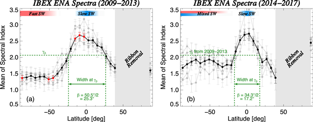
Figure 5. (a) IBEX ENA spectral index as a function of latitude for 2009–2013 (gray) and their weighted mean (black). The six directions in the sky that we use to calculate γβ are shown as red data points. (b) IBEX ENA spectral index as a function of latitude for 2014–2017 (gray) and their weighted mean (black). Angle β is calculated as half the width of the distributions at γβ (green).
Download figure:
Standard image High-resolution imageTo calculate the width of the spectral index distribution in Figure 5(a), we find the intersections of γβ with the time-averaged data on both sides of the spectral peak and determine the latitudes of these intersections (vertical dashed green lines; Figure 5(a)). Halving the angular width of this region yields β. The uncertainty in β is calculated by fitting two separate lines to the two IBEX data points nearest the intersection, including the extremes of their uncertainties, i.e., fit lines to [(θi, γi + σγi), (θi+1, γi+1 − σγi+1)] and [(θi, γi − σγi), (θi+1, γi+1 + σγi+1)], where θ is the latitude, σγ is uncertainty in spectral index γ, and γi < γβ < γi + 1. We solve these two linear equations for when the spectral index γ equals the half maximum value and then difference the θ-intercepts. Halving these differences yields the estimated uncertainty of β. We find β from 2009 to 2013 is 253 ± 210. Note that the uncertainty in γβ is much smaller than the difference in γi and γi+1.
For the latter years of IBEX observations (2014–2017), the latitudinal structure of the ENA spectral index is different, reflecting conditions closer to solar maximum (Zirnstein et al. 2017a, 2020). As shown in Figure 5, the spectral index at high latitudes in 2009–2013 is <1.5 and increases to ∼2.5 at low latitudes. However, in 2014–2017, the spectral index at high latitudes is more variable and, on average, is ∼1.8, reflecting a mixture of slow and fast SW during solar maximum. We argue that γβ found in 2009–2013 is also applicable to 2014–2017, since it should represent the average spectral index of ENAs produced from slow and fast SW, and thus reflects the latitude at which the spectrum is balanced by ENAs produced along distances A and B. If we take γβ found in 2009–2013 and apply it to the data taken in 2014–2017, we find that β is 172 ± 152. In Section 4 we discuss in more detail the origin of the spectral index observed in 2014–2017.
We note that the derivation of angle β from Equation (1) includes the effects of the differences in PUI energies of the slow versus fast SW plasma in the IHS. Differences in the ENA spectra at low versus high latitudes is direct evidence that the average PUI energy (or temperature) is different in the slow and fast SW, and thus is inherently taken into account in our analysis.
3.4. Distance to the TS and the Cooling Length—Distance C
We assume that the distances to the TS R1(α) ≅ R2(β). We make this assumption based on the TS geometry results presented by McComas et al. (2019). These authors derived the 3D TS geometry based on Voyager 1 and 2 observations of the TS crossings on the upwind side and magnetic disconnections from the acceleration source of anomalous cosmic rays on the downwind side of the TS. Based on their results, the distance to the TS at points R1 and R2 is approximately 160 au for both cases. We note that this distance is an estimate of the time-averaged distance to the TS. It is shown by Equation (1) that if the distance to the TS at the fast SW latitude is larger (R2 > R1), then the cooling depth distance will decrease. On the other hand, if R2 < R1, then the cooling depth distance will increase. If the dynamic pressure of the SW is largely independent of latitude, as derived from Ulysses observations (e.g., McComas et al. 2008), then the distance to the TS at different latitudes will be similar, as was assumed in our analysis. However, changes over time due to solar transients or during the transition from solar minimum to maximum may change this assumption (e.g., Pogorelov et al. 2017), but only if the changes occur over large enough timescales to affect the LOS-integrated ENA flux measurements. Therefore, for the time-averaged SW near solar minimum, we believe the assumption of R1 = R2 is a reasonable approximation. Uncertainties in the distance to the TS over time due to changes over the solar cycle are discussed in Section 4.
With these assumptions, we solve Equation (1) for B, yielding
where RTS = R1 = R2.
In order to calculate the distance to the ENA source, i.e., cooling length (Schwadron et al. 2014; Zirnstein et al. 2016a) C = A + B, next we need to solve for A. As stated earlier, one possible solution is that the ENA spectral index γβ shown in Figure 5 is produced when the LOS-integrated fluxes from the fast and slow SW are created along equal distances, i.e., A = B. However, this assumption ignores the fact that the energetic parent protons in the IHS experience an extinction effect from losses by charge exchange. This effect is important to consider since our goal is aimed at deriving the cooling length C which itself depends on the extinction effect by charge exchange. Therefore, one should set

where η = nHσ(v)v is the charge-exchange rate, nH is the neutral H density, σ is the energy-dependent, charge-exchange cross section (Lindsay & Stebbings 2005), v is the speed of ENAs, Lf and Ls are the average streamline distances from the TS to the IBEX LOS along A (in fast "f" SW) or B (in slow "s" SW), respectively, and u is the plasma flow speed for the fast or slow SW. The exponential terms represent the probability of survival by charge exchange. We make the approximation that ηf,s and uf,s are constant over the average streamline distances Lf,s.
To solve Equation (4), first we note that the rates of charge exchange depend on the dominant energy of ENAs from the slow and fast SW affecting the measured spectral index. Since we are calculating the spectral index over energy bins with central energies from 1.74 to 4.29 keV, we can reasonably assume that the measured ∼1.7 keV ENAs are dominated by ENAs created in the cooler, slow SW, and the measured ∼4.3 keV ENAs are dominated by ENAs created in the hotter, fast SW. Even though the slow SW also creates lower energy ENAs (<1.7 keV), these likely do not affect the spectral index calculated over 1.74–4.29 keV as much as ∼1.7 keV ENAs (see IBEX-Hi ESA response functions in Funsten et al. 2009). Therefore, the ratio of the charge-exchange rates in the fast and slow SW ηf/ηs = [σ(v)v]4.3 keV/[σ(v)v]1.7 keV ≅ 1.2.
The typical speed of the slow SW upstream of the TS is between ∼350 and 500 km s−1 and the typical speed of the fast SW is between ∼700 and 800 km s−1 (Figure 4), yielding a ratio range of 1.4 < uf/us < 2.3, and on average uf/us ≅ 1.85. The ratio uf/us will change in the IHS depending on the TS compression ratio. While there are no in situ observations of the TS in the direction of the heliotail, steady-state MHD simulations of the heliosphere suggest that the compression ratios at the upwind and downwind TS are similar (e.g., Zirnstein et al. 2018b; Heerikhuisen et al. 2019). The biggest differences between the upwind and downwind TS are their relative distances from the Sun due to the stagnating flow in the upwind direction and outflow in the downwind direction.
If we assume that the TS compression ratio for the slow SW in the downwind direction is similar to that observed by Voyager 2 (∼2.5; Richardson et al. 2008), and the compression ratio for the fast SW must be greater due to its higher Mach number (e.g., Fitzpatrick 2014), then the ratio of fast to slow SW speed in the IHS becomes smaller. We estimate this ratio by solving the ideal MHD jump conditions at a perpendicular shock. Using Voyager 2 observations, but scaling the proton density down to account for the longer distance to the downwind TS (84–160 au; McComas et al. 2019), we are able to acquire a compression ratio of ∼2.5 after adding a PUI population with 25% of the proton density and temperature of 4.7 × 10⁶ K. By substituting an SW speed 1.85 times faster than that observed by Voyager 2, the compression ratio increases to ∼3.4. With this higher compression for the fast SW, the ratio of fast-to-slow SW in the IHS is most likely 1 < uf/us < 1.7, and on average uf/us ∼ 1.4. Note that the compression ratio is in general determined from the ratio of densities across the TS, and only from the radial velocity component if the shock normal is radial. Since the TS is likely not Sun-centered nor strictly spherical, our analysis above has uncertainties depending on the actual orientation of the shock normal. However, given (1) the large uncertainties in our final results, (2) our derivation of the minimum distance to the ENA source, and (3) that the TS is more likely quasi-perpendicular than not at low-to-midlatitudes, this is likely a reasonable assumption for the purposes of our study.
Finally, the distances Lf and Ls are the average streamline lengths that the plasma takes to travel from the TS through the fast and slow SW, respectively, intersecting the LOS along A + B. Since A is located farther from the TS than B (see Figure 3(b)), it is obvious that Lf must always be greater than Ls. ENAs created along distance B originate from plasma parcels that travel different streamline distances from the TS to different points along B. One might assume that the average streamline distance Ls must connect to B at its halfway distance, such that X = B/2 in Figure 3(c). However, this is not necessarily true. A generalized solution for Ls can be calculated by assuming that the nearly triangular area between Ls, X, and the TS, Area1 ≅ (1/2)X (X + τ1)tanβ, equals half the entire area between min(Lf), B, and the TS, Area2 ≅ (1/2)B(B + τ1+ τ2)tanβ. By solving this condition, a set of equations can be derived to relate Ls and the minimum of Lf,
Solving Equations (5) for the ratio of min(Lf)/Ls yields
Here we show that  and thus A ≥ B. Knowing the ratios ηf/ηs = 1.2 and uf/us < 1.7, we find that for A ≥ B to be true, Lf/Ls > 1.7/1.2 ∼
  , which has been proven by Equation (6) for the minimum of Lf when we limit A = 0. Thus, as A increases, Lf must increase and Ls remains constant, and the condition Lf/Ls >
  is easily satisfied.
Therefore, instead of solving Equation (4) for A and estimating values for η, L, and u, we can reasonably assume that A ≥ B, yielding C = A + B ≥ 2B as a minimum for the cooling length of ENAs. Thus, C is given as
The uncertainty in C, σC, is calculated by the propagation of uncertainties for α (σα) and β (σβ), yielding
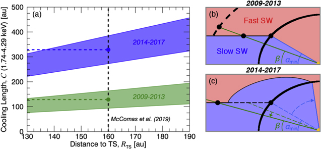
The solutions for Equations (7) and (8) are shown in Figure 6, where we set RTS as a free parameter. We also show the predicted distance to the TS in this particular direction from McComas et al. (2019), i.e., RTS = 160 au. With this distance, we find that C ≥ 129 ± 35 au in 2009–2013 and C ≥ 329 ± 56 au in 2014–2017. The total distances of the ENA source from the Sun are ≥289 ± 35 au and ≥489 ± 56 au, respectively. The increase in time of the distance to the ENA source is a potential indication of the motion of the ENA source down the heliotail.
Figure 6. (a) Minimum cooling length for 1.7–4.3 keV ENAs in the heliotail as a function of distance to the TS. Uncertainty in angle β is translated as the shaded green and blue regions. The predicted distance to the TS from McComas et al. (2019) is shown as the vertical dashed line. (b), (c) Illustration of the SW conditions during the two time periods. Note that the dashed lines in panel (c) represent the earlier conditions in panel (a). The black dashed curve representing the cooling length is beyond the margins of panel (c).
Download figure:
Standard image High-resolution image
4. Discussion and Conclusion
In this study we derived the minimum distance to the source of ∼1–6 keV ENAs in the heliotail, i.e., the minimum 1/e cooling length distance. This derivation is made possible by a combination of Ulysses SW observations and IBEX ENA observations. Our results are similar to previous model calculations (e.g., Schwadron et al. 2014; Zirnstein et al. 2016a), at least for IBEX observations made in 2009–2013. In this time period, we derived a distance from the Sun to the ENA source of ≥289 ± 35 au, assuming the distance to the TS is ∼160 au. However, the distance to the TS can change over time. While there are no direct observations of the TS in the downwind hemisphere, simulations suggest the downwind TS distance may change by ±10 au over the solar cycle (e.g., Izmodenov et al. 2005). In this case, our results for C would vary by an additional ±10 and ±24 au for the time periods 2009–2013 and 2014–2017, respectively.
Our analysis also assumes that the SW speed is constant from the Sun to the TS, which we used to determine the ratio of the SW speeds upstream of the TS, i.e., 1.4 < uf/us < 2.3. In reality, the SW slows down as a function of distance from the Sun due to mass-loading by the pickup of ionized interstellar neutral H atoms. To understand the effects of this assumption on our analysis, here we estimate the slowing of the SW speed using Equation (7) from Lee et al. (2009). First, we calculate the LOS-averaged interstellar neutral H density along the radial LOS of R1 and R2 by solving the hot model of interstellar neutral H (e.g., Thomas 1978) using the range of SW speeds from Ulysses observations, a time-independent photoionization rate at 1 au of 10−7 s−1 during solar minimum of cycle 23 (Sokół et al. 2020), and an interstellar neutral H density far from the Sun of ∼0.1 cm−3 (Bzowski et al. 2009). We find that the LOS-averaged interstellar neutral H densities are ∼0.06 cm−3 and ∼0.08 cm−3 along R2 and R1, respectively. By solving Equation (7) from Lee et al. (2009) to determine the rate of slowing of the SW, we estimate that the ratio of SW speeds upstream of the TS is changed to 1.2 < uf/us < 2.3, which is an insignificant change compared to our prior assumption. However, the interstellar neutral H density at high latitudes along R1 may be smaller than our prediction due to the fact that interstellar neutrals must travel through both slow and fast SW at high latitudes over long periods of time. For a slightly smaller neutral H density of ∼0.07 cm−3 along R1, the ratio of upstream SW speeds only slightly changes to 1.2 < uf/us < 2.4. Therefore, the change in the SW speed ratio is small compared to the uncertainties of our main results.
We showed that the ENA source distance increases by ∼100–300 au from 2009–2013 to 2014–2017, suggesting a motion of the ENA source over time. This behavior indicates a more complex, but realistic, picture of the heliotail. As shown by time-dependent simulations of the heliosphere (e.g., Pogorelov et al. 2015; Zirnstein et al. 2017b), the evolution of the solar cycle produces cyclical layers of fast/hot and slow/cool SW plasma parcels that propagate down the heliotail. Initially during solar minimum when the PCHs are open and the fast SW is emitted at the lowest possible latitude, the fast–slow SW structure maintains its height above the equatorial plane as it propagates away from the TS (Figure 3), which is what IBEX observed in 2009–2013.
As the solar cycle evolves toward maximum, the PCHs close and the fast SW is no longer emitted at midlatitudes (except for fast SW emitted from small coronal holes at all latitudes during solar maximum, but their SW speed is slower on average due to stream interactions). Slower SW fills in the heliotail, and the midlatitude fast SW that was a remnant of solar minimum travels down the heliotail and in effect produces a smaller elevation angle β, effectively producing what IBEX observes in 2014–2017. These two situations are illustrated in the right panels of Figure 6. Moreover, the quasi-periodicity of the SW suggests that the behavior observed by IBEX is repetitive. In fact, we predict that the distance to the ∼1–6 keV ENA source from the fast SW in the heliotail will decrease again in coming years, perhaps back to a distance similar to that measured in 2009–2013.
Finally, we note that our analysis assumed that the SW immediately propagates downwind (parallel to the equatorial plane) upon crossing the TS. In reality, the SW will have a radial component downstream of the TS for a period of time before being directed downwind. If the SW flow velocity maintains a radial component for a certain period of time, it would travel to higher distances from the equatorial plane (in Figure 3(b), L1 increases) before its propagation is directed downwind only, effectively increasing angle β. The distance to the ENA source would need to be farther away from the Sun to produce the same angle β observed by IBEX. Thus, the results in this study give a lower limit to the distance to the ENA source under this scenario.
This work was funded by the IBEX mission as a part of the NASA Explorer Program (80NSSC20K0719). Ulysses SW data was extracted from the SPDF (https://spdf.gsfc.nasa.gov/). J.M.S. acknowledges support by the Polish National Agency for Academic Exchange (NAWA) Bekker Program Fellowship PPN/BEK/2018/1/00049. E.Z. thanks Jacob Heerikhuisen for helpful discussions.