The Role of Turbulence for Heating Plasmas in Eruptive Solar Flares

Jing Ye; Qiangwei Cai; Chengcai Shen; John C. Raymond; Jun Lin; Ilia. I. Roussev; Zhixing Mei

doi:10.3847/1538-4357/ab93b5

1. Introduction

In the process of a moderately large solar eruption, about 10³² erg of energy is released and converted into kinetic and thermal energy via magnetic reconnection (Forbes 2000). The standard flare model, also named by the CSHKP scenario (Carmichael 1964; Sturrock 1966; Hirayama 1974; Kopp & Pneuman 1976), describes the overall evolution of eruptive flares, where two oppositely directed outflow jets are intermittently produced. In this model, a long current sheet (CS) develops connecting to the flare arcade, and various magnetic reconnection processes take place within.

The famous Sweet–Parker model (Parker 1957; Sweet 1958) predicts a reconnection rate too slow to explain the rapid release of energy that is observed, while the Petschek model (Petschek 1964) describes a single X-point configuration of the diffusion region allowing for fast reconnection. As far as the tearing instabilities (Furth et al. 1963) are concerned, it has been widely accepted that magnetohydrodynamic (MHD) turbulence plays a key role in quickening the energy dissipation in the reconnection CS (Lin et al. 2007; Loureiro et al. 2007). The CS fragmentation and cascading reconnection in solar flares was exhaustively studied by Bárta et al. (2011) using high-resolution simulations, and they gave the magnetic energy distribution along the CS a spectral index of −2.14. As suggested by Lazarian et al. (2020), turbulence requires the energy to cascade into smaller scales. Hence, the fragmented CSs and plasmoids in two dimensions belong to turbulence, while the inverse cascade of merging loops does not. Dong et al. (2018) also point out that the standard inertial range is characterized by a spectral index of −1.5, and it becomes steeper than the Kolmogorov spectrum because of the copious formation of plasmoids in the CS. However, the mechanisms with respect to turbulence for the fast energy dissipation and eventual heating of plasmas in specific regions are still far from being fully understood.

Our previous 2.5D numerical experiments suggest that there are three kinds of turbulence existing in solar eruptions if a CS develops long enough (Ye et al. 2019b). They are located inside the CS, at the bottom of a coronal mass ejection, and above the top of a flare loop, respectively. The turbulence inside the CS, which attracts much attention from the scientific community, is believed to be the result of the instability of plasmoids causing a large number of small, transient local diffusion regions (Shibata & Tanuma 2001; Loureiro et al. 2007; Shen et al. 2013; Ni et al. 2015). In addition, Drake et al. (2019) recently claimed that electrons can be accelerated in the reconnecting CS by turbulence at MHD scales. Consistent with the flare observations, the acceleration is the first-order Fermi regime dominated and energetic particles spread over broad regions instead of the boundary layers of a single, large-scale reconnection site. This suggests contracting magnetic islands. Recent spectroscopic observations of a CS related to the X-8.2 class solar flare on 2017 September 10 reported, for the first time, by Li et al. (2018) suggested that turbulent features in the CS can provide a very efficient route for the diffusion process. Later, Cheng et al. (2018) analyzed this event in detail and found that plasmas converge toward both sides of the CS, resulting in significant plasma heating and nonthermal motions. The radiation intensities of the outflow jets in different extreme ultraviolet (EUV) passbands also show a power-law distribution in the spatial- and temporal-frequency domain. So, solid evidence of the fragmented and turbulent magnetic reconnection occurring inside the CS was directly found through observations.

The turbulence above the flare loop-top is equally important for fast energy dissipation. Takahashi et al. (2017) suggested quasiperiodic transverse oscillations above the flare loops due to reconnection jets. Takasao & Shibata (2016) found that the local oscillations in this region consist of quasiperiodic propagating fast-mode magnetoacoustic waves. Additionally, the Kelvin–Helmholtz instability is argued to be a novel ingredient of the turbulence at the flare loop-top owing to chromospheric evaporation (Fang et al. 2016; Ruan et al. 2018). Many observations (McKenzie & Hudson 1999; McKenzie 2000; Reeves & Golub 2011; Hanneman & Reeves 2014; Innes et al. 2014) reported diffuse regions of hot, 10 MK plasma above the flare loops, namely supra-arcade fans (SAFs). And the turbulence mentioned could be colocated with a part of SAFs between the bottom of the CS and the top of flare loops. In SAFs, hard X-ray (HXR), radio, and microwave emissions often take place. Using RHESSI, Gallagher et al. (2002) found, for the first time, that the 12–25 keV source coincided with the site of the SAF identified by the Transition Region and Coronal Explorer 195 band from the edge-on perspective. Polito et al. (2018) and Gary et al. (2018) analyzed the existence of the HXR and nonthermal microwave source in the SAF from their observational work. Also, Cai et al. (2019) restudied the flare event on 2017 September 10 and suggested that the SAF possibly contains the termination shock (TS). Therefore, the study of the relationship between the turbulence above the flare loops and the formation of the SAF is indispensable for providing a better understanding of the source of the HXR and microwave emission.

In the present work, we focus on the plasma heating processes via turbulence inside the CS and above the loop-top as well as their interplay, considering the CSHKP configuration, and we use high-resolution MHD simulations with realistic thermal conduction and radiative cooling included. With an appropriate setup, we are able to analyze the fine thermal structures in the corona and build a series of synthetic images to compare directly with observations. This helps us to better understand the emission features possibly related to turbulence in a more detailed view.

The paper is organized as follows. Section 2 describes the numerical model and the initial setup as well as substantial improvements on numerical methods to make the simulations more efficient and stable. The numerical results of the global evolution, properties of turbulence at different locations, as well as synthetic images in multiple passbands are presented in Section 3. Lastly, the discussion and conclusions are summarized in Section 4.

2. Numerical Model Description

The MHD simulation investigated here is the classic standard flare model formalized by Kopp & Pneuman (1976). The evolution of the system can be adequately described by a 2.5D magnetic disruption MHD model including gravity, resistivity, thermal conduction, and radiative cooling in Cartesian geometry:

$\begin{eqnarray}&&\displaystyle \frac{\partial \rho }{\partial t}+{\rm{\nabla }}\cdot (\rho {\boldsymbol{v}})=0,\end{eqnarray} \tag{ 1 }$

$\begin{eqnarray}&&\begin{array}{l}\displaystyle \frac{\partial e}{\partial t}+{\rm{\nabla }}\cdot \left[(e+{P}^{* }){\boldsymbol{v}}-({\boldsymbol{v}}\cdot {\boldsymbol{B}}){\boldsymbol{B}}\right]\\ \ =\ \rho {\boldsymbol{g}}\cdot {\boldsymbol{v}}+{\rm{\nabla }}\cdot \left[\eta {\boldsymbol{B}}\times ({\rm{\nabla }}\times {\boldsymbol{B}})+{\kappa }_{| | }({\rm{\nabla }}T\cdot \hat{{\boldsymbol{B}}})\hat{{\boldsymbol{B}}}\right]\\ \quad \ -\ {n}_{i}{n}_{e}Q(T)+H,\end{array}\end{eqnarray} \tag{ 2 }$

$\begin{eqnarray}&&\displaystyle \frac{\partial (\rho {\boldsymbol{v}})}{\partial t}+{\rm{\nabla }}\cdot \left[\rho {\boldsymbol{vv}}-{\boldsymbol{BB}}+{P}^{* }{\boldsymbol{I}}\right]=\rho {\boldsymbol{g}},\end{eqnarray} \tag{ 3 }$

$\begin{eqnarray}&&\displaystyle \frac{\partial {\boldsymbol{B}}}{\partial t}={\rm{\nabla }}\times ({\boldsymbol{v}}\times {\boldsymbol{B}}-\eta {\rm{\nabla }}\times {\boldsymbol{B}}),\end{eqnarray} \tag{ 4 }$

$\begin{eqnarray}&&{P}^{* }=P+\displaystyle \frac{{\boldsymbol{B}}\cdot {\boldsymbol{B}}}{2},\end{eqnarray} \tag{ 5 }$

$\begin{eqnarray}&&P=\rho T.\end{eqnarray} \tag{ 6 }$

All the variables are dimensionless, where ρ is the plasma mass density, n_i and n_e are the number density of ions and electrons, v is center of mass velocity, P is the gas pressure, B and $\hat{{\boldsymbol{B}}}$ are the magnetic field and the associated unit vector, γ = 5/3 is the ratio of specific heat, e = P/(γ − 1) + ρ v²/ 2 + B · B/2 is the total plasma energy per unit volume (including thermal energy, kinetic energy, and magnetic energy), η is the resistivity, and g is the gravitational acceleration. The anisotropic conductivity coefficient ${\kappa }_{| | }$ is given by Spitzer theory (Spitzer 1962):

$\begin{eqnarray}&&{\kappa }_{| | }={c}_{1}\cdot \displaystyle \frac{1.84\times {10}^{-10}({{\rm{W}}/{\rm{m}}/{\rm{K}}}^{7/2})}{{\rm{ln}}{\rm{\Lambda }}}{T}^{5/2},\end{eqnarray} \tag{ 7 }$

with ln Λ the Coulomb logarithm set to 30, the normalization factor ${c}_{1}={\mu }_{0}{T}_{c}^{7/2}/({B}_{c}^{2}{L}_{c}{v}_{A})$ . Here, T_c, B_c, L_c and ρ_c are the normalization units for temperature, magnetic field, length and mass density, respectively. The Alfvén speed is thus ${v}_{A}={B}_{c}/\sqrt{{\mu }_{0}{\rho }_{c}}$ , where μ₀ = 4π × 10⁻⁷ H m⁻¹. And the Lundquist number is defined as S = 1/η. The radiative cooling rate Q(T) for fully ionized hot plasma is given as described in Klimchuk et al. (2008):

$\begin{eqnarray}&&\begin{array}{l}Q(T)\ =\\ \left\{\begin{array}{lll}1.09\times {10}^{-31}{c}_{2}{(T\cdot {T}_{c})}^{2} & \mathrm{for} & T\leqslant {10}^{4.97}/{T}_{c},\\ 8.87\times {10}^{-17}{c}_{2}{(T\cdot {T}_{c})}^{-1} & \mathrm{for} & {10}^{4.97}/{T}_{c}\lt T\leqslant {10}^{5.67}/{T}_{c},\\ 1.90\times {10}^{-22}{c}_{2} & \mathrm{for} & {10}^{5.67}/{T}_{c}\lt T\leqslant {10}^{6.18}/{T}_{c},\\ 3.53\times {10}^{-13}{c}_{2}{(T\cdot {T}_{c})}^{-3/2} & \mathrm{for} & {10}^{6.18}/{T}_{c}\lt T\leqslant {10}^{6.55}/{T}_{c},\\ 3.46\times {10}^{-25}{c}_{2}{(T\cdot {T}_{c})}^{1/3} & \mathrm{for} & {10}^{6.55}/{T}_{c}\lt T\leqslant {10}^{6.90}/{T}_{c},\\ 5.49\times {10}^{-16}{c}_{2}{(T\cdot {T}_{c})}^{-1} & \mathrm{for} & {10}^{6.90}/{T}_{c}\lt T\leqslant {10}^{7.63}/{T}_{c}\\ 1.96\times {10}^{-27}{c}_{2}{(T\cdot {T}_{c})}^{1/2} & \mathrm{for} & {10}^{7.63}/{T}_{c}\lt T.\end{array}\right.\end{array}\end{eqnarray} \tag{ 8 }$

and the heating function H is similar to Ni et al. (2015) in order to hold the static thermal equilibrium at the temperature T₀ for the background:

$\begin{eqnarray}&&H=3.53\times {10}^{-13}{n}_{i}{n}_{e}{c}_{2}{({T}_{0}\cdot {T}_{c})}^{-3/2},\end{eqnarray} \tag{ 9 }$

where T₀ = 0.0077 is the initial temperature in the corona and ${c}_{2}=1\times {10}^{-13}{\mu }_{0}{\rho }_{c}^{2}{L}_{c}/({M}_{p}^{2}{B}_{c}^{2}{v}_{A})$ is the normalization factor with M_p = 1.673 × 10⁻²⁷ kg the mass of the hydrogen atom. Note that the single background heating term H used in our simulation does not yield any evaporation condensation process in the corona. To complete the above equations, the divergence-free condition (∇ · B = 0) should be satisfied at all times of the evolution.

The normalization units are given as ρ_c = 1.673 × 10⁻¹² kg m⁻³, B_c = 0.003 T, L_c = 10⁸ m, and eventually we have the characteristic values P_c = 7.162 Pa, T_c = 2.595 × 10⁸ K, v_A = 2.069 × 10³ km ⁻¹ and t_A = L_c/v_A = 48.33 s for pressure, temperature, velocity, and time, respectively. The entire simulation domain ranges from −1 to 1 (L_c) in the x-direction, and from 0 to 2 (L_c) in the y-direction. The initial magnetic field of the CSHKP model reads as

$\begin{eqnarray}\begin{array}{rcl}{B}_{x} & = & 0,\\ {B}_{y} & = & \left\{\begin{array}{l}\sin \left(\displaystyle \frac{\pi x}{2\lambda }\right),\mathrm{if}\quad | x| \leqslant \lambda \\ 1,\quad \ \mathrm{else}.\end{array}\right.,\\ {B}_{z} & = & \sqrt{(1-{B}_{x}^{2}-{B}_{y}^{2})},\end{array}\end{eqnarray} \tag{ 10 }$

where λ is the half width of the CS set to 0.1. To have the system evolve from the initial quasi-steady state to a burst reconnection phase, we introduce a small perturbation on the magnetic potential as

$\begin{eqnarray}&&{A}_{\varepsilon }=\varepsilon \cdot \exp \left[-{\left(\displaystyle \frac{x}{{l}_{x}}\right)}^{2}-{\left(\displaystyle \frac{y-{y}_{c}}{{l}_{y}}\right)}^{2}\right],\end{eqnarray} \tag{ 11 }$

where ε = 0.01 is the magnitude of the noise, y_c = 0.5 is the perturbation center along the y-axis, and l_x = 0.05 and l_y = 0.05 are the nondimensional perturbation wavelengths in the x- and y-directions, respectively. Then, the x- and y-components on the magnetic field, denoted by B_εx and B_εy, can be easily deduced from the relation B_εx = ∂A_ε/∂y and B_εy = −∂A_ε/∂x.

We take the gravitational acceleration as ${\boldsymbol{g}}=-{c}_{3}{g}_{0}\hat{y}/{(1+{{yL}}_{c}/{R}_{\odot })}^{2}$ , with the solar radius R_⊙ = 6.961 × 10⁸ m, the gravitational acceleration near the solar surface g₀ = 274 m s⁻² and the normalization factor c₃ = ρ_cL_c/P_c. Here, $\hat{{\boldsymbol{y}}}$ is the unit vector in the y-direction. In order to handle the line-tied boundary condition at the bottom, we construct a two-layer atmosphere by a very high-density chromosphere (0 ≤ y ≤ h + 5w) and an isothermal corona (y > h + 5w) in the calculations, with h = 0.03 the height and w = 0.0075 the width of the transition region. The initial temperature distribution reads as:

$\begin{eqnarray}&&T(y)=\displaystyle \frac{({T}_{\mathrm{cor}}-{T}_{\mathrm{chr}})}{2}\tanh \left[(y-h)/w)\right]+\displaystyle \frac{{T}_{\mathrm{cor}}+{T}_{\mathrm{chr}}}{2},\end{eqnarray} \tag{ 12 }$

where T_cor = 7.71 × 10⁻³ is the temperature for the corona and T_chr = 1.66 × 10⁻⁵ is the temperature for the chromosphere. Hence, the gas pressure and the associated density distribution of hydrostatic equilibrium are given by

$\begin{eqnarray}&&P(y)={P}_{\mathrm{chr}}\exp \left[-{\int }_{0}^{y}\displaystyle \frac{{c}_{2}{g}_{0}}{T(y)}{\left(1+\displaystyle \frac{{{yL}}_{c}}{{R}_{\odot }}\right)}^{-2}{dy}\right],y\leqslant h+5w,\end{eqnarray} \tag{ 13 }$

$\begin{eqnarray}\begin{array}{rcl}P(y) & = & {P}_{\mathrm{cor}}\exp \left[\displaystyle \frac{{c}_{2}{g}_{0}{R}_{\odot }}{{T}_{\mathrm{cor}}{L}_{c}}\left(\displaystyle \frac{1}{1+{{yL}}_{c}/{R}_{\odot }}-\displaystyle \frac{1}{1+{h}_{c}{L}_{c}/{R}_{\odot }}\right)\right],\\ y & \gt & h+5w,\end{array}\end{eqnarray} \tag{ 14 }$

where

$\begin{eqnarray}&&{P}_{\mathrm{chr}}={P}_{\mathrm{cor}}\exp \left[{\int }_{0}^{h+5w}\displaystyle \frac{{c}_{2}{g}_{0}}{T(y)}{\left(1+\displaystyle \frac{{{yL}}_{c}}{{R}_{\odot }}\right)}^{-2}{dy}\right].\end{eqnarray} \tag{ 15 }$

The gas pressure at y = h + 5w is set to be P_cor = 0.058 and the plasma density at y = h + 5w is ρ = 7.61. Accordingly, the plasma β ≈ 0.116 at y = h + 5w. Since the gravitationally stratified solar atmosphere consists of two layers at different temperatures, the density of the thin chromosphere layer is calculated to be over two orders of magnitude larger than that in the corona. In this way, the line-tied condition is approximately satisfied with all parameters fixed near the bottom instead of being treated analytically as described by Forbes & Priest (1984), and one can remove the complicated behavior of plasmoids and the magnetic field near the bottom due to the low β environment (Mei et al. 2012). The chromosphere layer is thus maintained frozen and simply assumed to be always in the thermal equilibrium during the evolution (i.e., Q(T) = H for 0 ≤ y ≤ h + 5w), because we mainly focus on the structures in the corona.

The boundary conditions are as follows. The line-tied condition is used for the bottom boundary, and the other three boundaries, are open or free boundaries on which the plasma and the magnetic flux are allowed to enter or exit freely, as described in Shen et al. (2018) and Ye et al. (2019b).

2.1. Numerical Methods

The entire simulation is performed on ATHENA 4.2 (Gardiner & Stone 2005, 2008; Stone & Gardiner 2009). We have used the uniform grids of 2560 × 2560 and 3840 × 3840 for the same configuration with a Lundquist number S = 10⁶. In the present work, the hyperbolic MHD parts are solved by the Godunov method, where the shock structures are accurately captured using the Harten–Lax–van Leer discontinuities solver as described by Miyoshi & Kusano (2005) and Beckwith & Stone (2011). Under the circumstance that the local plasma β sometimes becomes extremely small (<10⁻⁵) in the computation, negative pressure or density begins to appear, which leads to a convergence failure at a later time. In order to preserve the positive monotonicity of our scheme, we used a practical approach in the same way as Balsara & Spicer (1999) to correct the unreasonable density or pressure. On the other hand, the parabolic thermal conduction part is solved by the novel semi-implicit method as described in Ye et al. (2019a).

Two uniform grids of 2560 × 2560 and 3840 × 3840 have been implemented for the high Lundquist number S = 10⁶ simulations. The general reconnection processes and magnetic fields of both cases are similar except the small-scale structures (plasmoids), which are sensitive to the numerical resolution. We found that the main numerical errors are located in regions with large current densities using the error estimation method in Shen et al. (2011). Accordingly, the effective Lundquist number for the coarse grid (i.e., 2560²) is shown to be of the order of ∼10⁵ near the principal X-point, while that for the finer grid (i.e., 3840²) can meet the physical requirement of S = 10⁶. In order to better perform the turbulent regime during reconnection, the following analyses are all based on the results from the higher resolution simulation of 3840 × 3840.

3. Simulation Results

3.1. General Evolution

In this section, we study the global evolution of the standard flare system in the gravitationally stratified solar atmosphere. Figure 1 presents the temperature (first row) and density (second row) distributions from t = 0 to t = 40t_A. At t = 0, the corona is isothermal with the initial temperature T_cor (=2 MK in the dimensional form) and the density distribution decays exponentially with height. Then, the CS has been heated rapidly to 5.29 × 10⁻² (corresponding to 1.37 × 10⁷ K in the dimensional form), as plasmoids appeared at early stages t = 16t_A. At t = 28t_A, the system evolves into the steady reconnection phase, the density distribution of the flare shows a cavity in the cusp structure, while the temperature does not. So the low-density cavity found here may be the main reason that the EUV emission in this region, namely the dimming region, becomes weaker than the surrounding flare loop structures in many observations. Meanwhile, the temperature in the CS is much higher than the surrounding corona environment and the upper part of the CS is marginally hotter than the lower part. In addition, we observe the individual flare-loop shrinkage with a speed of ∼1.25 × 10⁻³v_A leading to substantial energy release at this time, which makes the flare arcade (inner loops) even hotter, as suggested by the observations of Warren et al. (2018). In particular, part of the heat is conducted to the upper chromosphere along the magnetic field, leading to chromospheric evaporation to form the hot dense postflare loops (Takasao et al. 2015). And the maximum temperature in the CS is about 5.65 × 10⁻², while that in the flare loops is about 3.61 × 10⁻². Finally, at t = 40t_A, the massive plasmas accumulate and fill the inner loops of the flare. The maximum temperature in the CS decreases to 5.29 × 10⁻², while that in the flare loops decreases to 3.44 × 10⁻². This indicates that the flare and CS undergo a decay phase at later times.

The principal X-point, where the reconnection rate takes its maximum value, is observed to be located close to the newly formed flare loops during the entire evolution causing the energy partition asymmetry in the CS (Reeves et al. 2010). Figure 2 shows the main magnetic reconnection rate (black solid line) from t = 0 to t = 40t_A, calculated by γ(t) = v_in/v_A, where v_in is defined as the inflow velocity near the principal X-point and v_A is the local Alfvén speed. And the red dashed line is the associated smooth distribution. As we can see, the reconnection rate rises drastically after about t = 16t_A due to plasmoid instability development and stabilizes at the level of ∼0.1 afterwards, which is consistent with the previous work by Shen et al. (2011).

**Figure 2.** Magnetic reconnection rate γ (t) vs. time (black solid line) and the associated fitting curve (red dashed line).
Download figure:
Standard image High-resolution image

We investigate radiation energy and conduction flow in the simulation, including energy flow into and out of specific regions of interest. By integrating both sides of Equation (2) over a fixed volume V and applying the divergence theorem, the energy flow is:

$\begin{eqnarray}&&\begin{array}{l}{\displaystyle \int }_{V}\displaystyle \frac{\partial }{\partial t}({ \mathcal E }+{ \mathcal K }+{ \mathcal W }){dV}\\ =-{\displaystyle \int }_{V}({n}_{i}{n}_{e}Q(T)-H-\rho {\boldsymbol{v}}\cdot {\boldsymbol{g}}){dV}\\ -\ {\displaystyle \int }_{S}\left[\left(\displaystyle \frac{\gamma P}{\gamma -1}+\displaystyle \frac{\rho {v}^{2}}{2}\right){\boldsymbol{v}}+{\boldsymbol{E}}\times {\boldsymbol{B}}\right.\\ \left.-{\kappa }_{| | }({\rm{\nabla }}T\cdot \hat{{\boldsymbol{B}}})\hat{{\boldsymbol{B}}}\right]\cdot d{\boldsymbol{S}},\end{array}\end{eqnarray} \tag{ 16 }$

where ${ \mathcal E }$ , ${ \mathcal K }$ , and ${ \mathcal W }$ are the internal, kinetic, and magnetic energy densities, and E = η J − v × B is the electric field. The volume V is chosen to be [−0.3, 0.3] × [0.105, 2] (white box in Figure 1(d)), which covers the entire evolution of flares and CSs in the corona. We have computed the conductive losses ${\int }_{S}{\kappa }_{| | }({\rm{\nabla }}T\cdot \hat{{\boldsymbol{B}}})\hat{{\boldsymbol{B}}}\cdot d{\boldsymbol{S}}$ and radiative losses ${\int }_{V}{n}_{i}{n}_{e}Q(T){dV}$ as well as coronal heating ${\int }_{V}{HdV}$ in cgs units by multiplying the relevant characteristic values (also converted into cgs units) for the simulations. Note that the integrations here take account of the normalized length of 1 along the line of sight as well. The results are plotted in Figure 3. In panel (a), the evolution initiates from the thermal equilibrium state, the radiative losses are marginally larger than the coronal heating at early stage (t ≤ 20t_A), while the heating dominates when a tearing-mode instability develops (t > 20t_A). The domination at later times is because the dense plasma accumulates with the reconnected magnetic flux in the flare loops and the cooling rate could be relatively smaller than the heating rate once the CS and the flare become hot (>10^6.55 K). Since conductive losses on the left and right sides of the volume V are negligible, we only calculated that on the top and at the bottom. The conductive losses become significant at both sides from t = 20t_A. The sign of the heat flux indicates that the heat flows into or out of the region of interest. One can find that the heat flux flows freely into or out of the boundary y = 2 (top) due to the open boundary setup, while an amount of heat flux comparable with the radiative losses goes downwards to the chromosphere along the magnetic lines of flare loops at y = 0.105 (bottom). Also, we calculated the intensities of total conductive losses and radiative losses on V. One can find in panel (b) that radiative losses of the order of 10⁷ erg cm⁻² s⁻¹ dominate for the main part of evolution. As the temperature rises through reconnection, conductive losses become important, even larger than the radiative losses. Our results are different to Raftery et al. (2009), because we take into account the energy losses in both the flare loops and the CS.

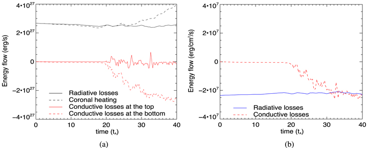
**Figure 3.** (a) Conductive losses on the top and at the bottom (red) of the volume V, coronal heating and radiative losses (black) over V; (b) conductive loss ratio ${\int }_{S}{\kappa }_{| | }({\rm{\nabla }}T\cdot \hat{{\boldsymbol{B}}})\hat{{\boldsymbol{B}}}\cdot d{\boldsymbol{S}}/V$ (dashed line) vs. radiative loss ratio ${\int }_{V}{n}_{i}{n}_{e}Q(T){dV}/V$ (solid line).
Download figure:
Standard image High-resolution image

**Figure 3.** (a) Conductive losses on the top and at the bottom (red) of the volume V, coronal heating and radiative losses (black) over V; (b) conductive loss ratio ${\int }_{S}{\kappa }_{| | }({\rm{\nabla }}T\cdot \hat{{\boldsymbol{B}}})\hat{{\boldsymbol{B}}}\cdot d{\boldsymbol{S}}/V$ (dashed line) vs. radiative loss ratio ${\int }_{V}{n}_{i}{n}_{e}Q(T){dV}/V$ (solid line).
Download figure:
Standard image High-resolution image

3.2. Interaction between Multiple TSs and Plasmoids

TSs have been predicted in a standard flare model, which allows for the generation of high-energy particles at the loop-top (Guo & Giacalone 2012). They may also play an important role in heating plasmas in or above the postflare loops (Masuda et al. 1994; Guidoni et al. 2015). In this subsection, we investigate the formation of multiple TSs at the loop-top and the dynamics of turbulence in the steady reconnection phase. We extracted four successive images from the original data to follow two plasmoids disrupting the structures of TSs and merging into the flare loops. In Figure 4, we plot the divergence of velocity, the fast magnetosonic Mach number, the current density, as well as the temperature at t = 27.8, 28, 28.2, 28.4t_A. Note that the Mach number is defined as ${v}_{\mathrm{flow}}/\sqrt{{c}_{s}^{2}+{v}_{\mathrm{AL}}^{2}}$ , where v_flow is the local velocity, c_s is the speed of sound, and v_AL is the local Alfvén speed. In Figure 4(a), a single TS is formed at y ≈ 0.43 before the merge begins. In panel (b), the first plasmoid begins to interact with the flare loops, and shock structures of the same strength driven by the plasmoid are formed at the interface near y = 0.46. Multilayer TSs appear above the flare loops before the collision. We also notice that the velocity along the y-axis underwent two phases of deceleration at the spots of TSs from our simulations. Then in panel (c), the first plasmoid finished the collision and a weaker TS reforms behind at y ≈ 0.45. Lastly, panel (d) is the very moment when the second plasmoid is crossing the TSs and the fast shocks driven by plasmoids are interacting with the loop-top. In Figures 4(e)–(h), we plot the Mach number variations which are larger than 1. At t = 27.8t_A, we see a lower Mach number at the cores of the plasmoids because of a higher pressure and magnetic field than the ambient downflows. The Mach number takes its maximum at the height y ≈ 0.43 and manifests as a slightly lower Mach number valley (1.6–1.8) near the shock front. As the plasmoid is approaching the TSs at t = 28t_A, the supermagnetosonic outflow passes the first TS and stops at the second TS beneath it. After the formation of the new TS at t = 28.2t_A, the Mach number near the shock front resumes to 1.4–1.6. At t = 28.4t_A, the plasmoid has destroyed the geometry of the TS and flows downward submagnetosonically. Also, we plot the current distribution perpendicular to the plane J_z = ∇ × B in panels (i)–(l), and one can see the turbulent reconnection proceeding constantly in thin CSs above the flare loops. In particular, the collision in panel (l) yields many small-scale fragmented CSs. Panels (m)–(p) show the associated temperature distributions. One can find in panel (o) that the turbulent region is compressed and heated by the collision, which may produce the intermittent enhancement found in soft X-rays (SXR) fluxes as well as sometimes in HXR, as reported in Liu et al. (2013). Together with panels (j)–(k), CSs above the flare loops might somewhat heat themselves, but substantial heating is provoked by the plasmoid collision.

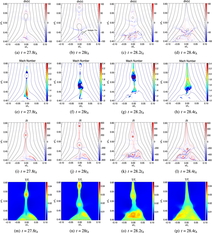
**Figure 4.** Two plasmoids merge continuously into the flare loops from t = 27.8t_A to t = 28.4t_A. The first row shows the divergence of velocity; the second row presents the magnetosonic Mach number (≥1); the third row shows the current density; the fourth row shows the associated temperature.
Download figure:
Standard image High-resolution image

In order to study the energy cascade using a 1D Fourier transform, we choose a strip in −0.0029 < x < 0.0029 which contains 10 numerical cells and calculate the averaged B_x as well as the spectrum of magnetic energy ${B}_{x}^{2}/2$ . As shown in Figure 5, the first row represents the associated 1D distributions of B_x at the above specific times, and the null points indicate the small-scale plasmoids. In the second row, the spectral index is α = −2.15 ± 0.025 at t = 27.8t_A before the collision, then that is α = −2.086 ± 0.026 at the beginning of the collision at t = 28t_A. After the collision, the spectral index returns to α = −2.101 ± 0.025 as plotted at t = 28.2t_A. And the spectral index drops to α = −1.826 ± 0.022 in the middle of the collision at t = 28.4t_A, when the TS collapses into multiple small-scale structures. Note that the wavenumber k reveals the distribution of the magnetic energy in different scales and is normalized by the characteristic length L_c. The larger k is, the smaller the structural scale becomes. When one TS is destroyed into pieces by plasmoids, the magnetic spectrum becomes softer (or flattened). In Figure 5(d), it can be seen that small-scale structures are more located in loop-top regions than in the higher part of the CS, so the softer index is likely dominated by TS relative structures. This indicates that the energy can cascade in a more efficient way, while the region above the flare loops becomes more turbulent.

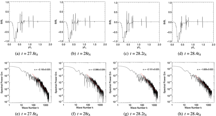
**Figure 5.** The first row shows the distribution of B_x along the y-axis in the center of the CS at t = 27.8, 28, 28.2, 28.4t_A; the second row shows the associated spectrum distribution using the 1D FFT technique.
Download figure:
Standard image High-resolution image

Previous spectral studies show that the turbulence inside the CS is anisotropic in the steady reconnection phase because the associated spectral indices are steeper than the Kolmogorov spectrum (=−5/3) for the magnetic energy perpendicular to the local magnetic field (Lazarian & Cho 2005). However, we have zoomed in on a square box of [−0.05, 0.05] × [0.4, 0.5] above the flare loops and calculated the magnetic spectrum ${{EB}}_{k}({kx},{ky})=({\tilde{B}}_{x}^{2}({kx},{ky})+{\tilde{B}}_{y}^{(}{kx},{ky})+{\tilde{B}}_{z}^{2}({kx},{ky}))/2$ , thereby using the 2D fast Fourier transform (FFT) technique at t = 16t_A (onset of plasmoid instability) and 28t_A (steady reconnection phase). Here, we define kx = 0, 2π/L_x, 2 × 2π/L_x, 3 × 2π/L_x, etc. and ky = 0, 2π/L_y, 2 × 2π/L_y, 3 × 2π/L_y, etc., with L_x = L_y = 0.1L_c the length scales selected in the x- and y-directions. In order to better display the 2D Fourier spectra, we have shown the imaginary parts of the spectra with negative coordinates as well. Figure 6 presents the distribution of lg(EB_k) for both times. At the early phase of reconnection t = 16t_A, the distribution of the power spectrum is peaked mainly at small kx, ky in the center, because no small structures have appeared. At a later phase of reconnection t = 28t_A, the spectrum spreads out to the larger kx, ky, indicating that smaller-scale structures are generated. And, the distribution of large log-scale values at t = 28t_A seems quasi-symmetric with reference to the diagonal. This means that the plasma in this region is roughly isotropic, probably due to the lack of an effective constraint by the magnetic field. Together with the inference from Figure 5, when the CS is well developed, the turbulence becomes simultaneously anisotropic and isotropic at different locations.

**Figure 6.** Log-scaled power spectrum from Fourier analysis of the magnetic energy in the turbulent region zoomed by the box of [−0.05, 0.05] × [0.4, 0.5].
Download figure:
Standard image High-resolution image

3.3. Synthetic Images

Since thermal conduction and radiative cooling mechanisms are included, the predicted temperature distribution should be more reliable than the simulations of Cai et al. (2019). We have used the density and temperature from the simulations to produce EUV images with the help of the CHIANTI database (Dere et al. 1997; Zhao et al. 2019). The synthetic observations for AIA 94, 131, 171, 304, and 193 Å are provided, which cover the temperature range in the corona. Figure 7 and the corresponding animation show the entire evolution in EUV images. And the bright CS and plasmoids are easily identified in the 94 and 131 Å channels. In particular, the heating effect underneath the TS after collision for t = 28.2t_A and turbulent structures above the loop-top for t = 28.4t_A can only be recognized in these two passbands.

Figure 7. SDO/AIA synthetic views in 94 Å, 131 Å, 171 Å, 304 Å, and 193 Å at t = 28.2 and 28.4t_A. An animation of EUV images in the associated passbands from t = 0 to t = 40t_A is available.

(An animation of this figure is available.)

Download figure:

Video Standard image High-resolution image

We are also interested in how the turbulence affects the above passbands in terms of radiation intensity. The distributions of the spectrum for t = 28.4t_A are calculated using a 1D FFT technique on their averaged intensity variations in the strip of −0.0014 < x < 0.0014. The intensity variation in each passband is defined as the intensity compared to its maxima and the wavenumber k is normalized by the characteristic length L_c. In Figure 8, the spectrum shows a power-law distribution with the spectral index of α = −1.864 ± 0.024 for AIA 94 Å, α = −1.338 ± 0.024 for AIA 131 Å, α = −0.963 ± 0.022 for AIA 171 Å, α = −1.345 ± 0.020 for AIA 304 Å, and α = −1.372 ± 0.023 for AIA 193 Å, respectively. So, the AIA 94 Å channel recognizes the most small-scale structures in the reconnecting CS as well as above the flare loops, because its spectral index is very close to that of the magnetic energy in Figure 5(h). And the AIA 131 and 193 Å channels give spectral indices similar to Cheng et al. (2018), which confirms the implication of fragmented and turbulent reconnection taking place in their observations.

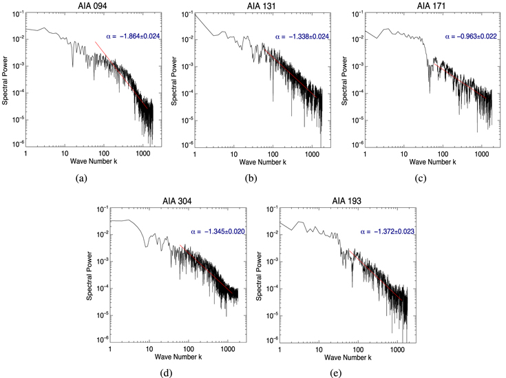
**Figure 8.** Spectrum distributions of radiation intensity in the passbands: (a) 94 Å; (b) 131 Å; (c) 171 Å; (d) 304 Å; (e) 193 Å.
Download figure:
Standard image High-resolution image

Following the approach of the synthetic spectral line given by Guo et al. (2017), we also obtained the synthetic emission line profiles of the Fe xxi 1354.08 Å line to study the turbulent motion in the CS based on the numerical results. In our calculation, the line broadening includes the thermal broadening and the instrument broadening (Innes et al. 2015; Guo et al. 2017). The thermal broadening of the Fe xxi line is obtained at 10^7.05 K, which corresponds to the peak of the ionization fraction curve of the Fe xxi ion, which is about 57.8 km⁻¹. We first interpolate the simulated profiles on the grid of 3840 × 3840 to the coarse grid of 1600 × 1600, of which the cell length is similar to the pixel size of the Interface Region Imaging Spectrograph (IRIS). Then, we use the contribution function of the ion of interest given by CHIANTI to calculate the spectral line under the assumption of the Gaussian distribution of the relative velocity. In addition, Fe xxi is assumed to be in ionization equilibrium in our case. By applying a single Gaussian fitting procedure to the spectral lines, we give the Doppler width as a function of the location of the CS in Figure 9. At the early stage of plasmoid instabilities t = 16t_A, the general line width distribution along the CS is close to the theoretical thermal width. At later times t = 28, 30t_A, the Doppler width varies from 57.8 to 97.5 km s⁻¹ and is larger at the location of plasmoids than the other places inside the CS, which is mainly related to the nonuniform distribution of density, temperature, and velocity near the plasmoids.

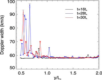
**Figure 9.** The Fe xxi 1354.08 Å Doppler width as a function of the location of the CS at t = 16, 28, 32t_A.
Download figure:
Standard image High-resolution image

The mechanism of quasiperiodic pulsations (QPPs) in flare light curves is also a controversial topic (McLaughlin et al. 2018). Many possibilities are considered, such as the oscillatory reconnection inflow (Nakariakov & Zimovets 2011; Santamaria et al. 2015), inherent periodicity of the reconnection (Takasao et al. 2015), or recently Kelvin–Helmholtz turbulence at the loop-top (Ruan et al. 2018). Instead of computing the entire flare emission, we are most interested in the turbulent region above the flare loops, in order to compare with the SAF observations in Cai et al. (2019). In this simplified model, a part of the SAF is believed to be located between the flare loop-top and the bottom of the CS, which is induced by the perturbation under the TSs. To exclude the primary emission from the loops, we automatically determined the position of the strongest TS, and then used it as the upper side of a box with a size of 0.05 × 0.05. The light curves are thus obtained by integrating the radiation intensities over that box. Figure 10 shows the light curves in cgs units for the AIA 94, 131, 171, and 304 Å channels from t = 10t_A to t = 35t_A. The profiles for AIA 94 Å and 131 Å successively increase and decrease for different reconnection phases, while the others monotonically decrease in general. According to our experiments, the maximum value in AIA 94 Å indicates the very moment when the temporal averaged density of the box in the SAF reaches its maximum, while that in AIA 131 Å is the timing when the average temperature reaches the maximum. This might be the essential fact responsible for the delay between the two passbands. In particular, the ups and downs in the decreasing phases of the AIA 94 and 131 Å channels imply plasmoid collisions with the TS and subsequent relaxation giving rise to the change in density and temperature, respectively. Our simulated results provide reliable time-dependent light curves in the SAF during the specific flare event, given the range of parameters and the line of sight integration, and we expect to confirm it by observation data in the future.

**Figure 10.** Synthetic light curves of the AIA 94, 131, 171 and 304 Å channels in the turbulent region above the loop-top from t = 10t_A to t = 35t_A.
Download figure:
Standard image High-resolution image

Before studying the QPPs in light curves, we first examine the temporal distribution of the horizontal velocity V_x averaged in the above box with the size of 0.05 × 0.05, which shows a quasiperiodic transverse oscillation after the plasmoid instability starts to develop from t = 16t_A in Figure 11(a). The wavelet spectrum based on the Morlet transform is given in Figure 11(b), where the black solid line indicates the significance levels. Then in Figure 11(c), the dashed line is the 95% significance level and the largest power value corresponds to a period of ∼1.39t_A, which is the dominant period of the oscillation above the loop-top. Since the peaks in the reconnection rate (Figure 2) indicate the generation of plasmoids, the difference between the reconnection rate and its smooth profile also shows periodicity, and the dominant period is 1.17t_A. In order to look into the oscillating features of the SAF, we extract the normalized fast-variation component (FVC) from the light curves in Figure 10. We first deduce the smooth trend of the light curves, then subtract the smoothing profiles from the original light curves and normalize the results by their maxima as shown in Figure 12. Indeed, the AIA 171, 304 Å channels reveal the periodic oscillations at the early time before plasmoid instability becomes severe, while the AIA 94, 131 Å channels show the quasiperiodic dynamics at later times. Applying the wavelet analysis to the normalized FVCs, the associated periods of QPPs are reported in Table 1. Interestingly, the AIA 94 and 131 Å channels of high temperature both possess two dominant periods, which identify the peaks of the power in the relevant 95% significance region. Taking AIA 94 Å for example, the period of 1.39t_A might be due to the intermittent heating by TSs, while the larger period of 2.34t_A is possibly related to the substantial contribution to heating by plasmoid collisions. And the case of the AIA 131 Å is similar. On the other hand, the AIA 171 and 304 Å channels of low temperature have an identical period of 1.65t_A, which principally reveals the change of density compressed by reconnection jets and plasmoids. Also, the associated physical time of QPPs in EUV images of the SAF generally agrees with the period of the oscillation features found in the IRIS slit-jaw images reported by Cai et al. (2019). Besides, Hayes et al. (2019) suggest that the kink mode can be connected to the QPPs, which oscillates in the vertical polarization leading to density perturbations. Following their interpretation for the kink mode, we obtained an internal Alfvén speed of the loop of ∼1418 km s⁻¹ considering the period of 79.74 s in AIA 131 Å and the loop length of ∼80 Mm (in Figure 1(c)) in our model. This theoretical velocity is a little larger than the simulated one, but still reasonable for coronal loops. Unlike Tan et al. (2007) and Tan (2008), the tearing-mode oscillations have a period of 1.17t_A from our simulation, which is not in agreement with the QPPs observed in Table 1. Thus the vertical kink-mode oscillations might be the main component in the turbulent region above the loop-top and are likely related to the interaction between plasmoids and the top of flare loops. From Figures 4(e)–(h), the change of the fast magnetosonic Mach number indicates the periodic variation of the compression ratio of TSs. The MHD oscillations on density and temperature could be the underlying mechanism responsible for the impulsive energy release in the QPPs, which is also suggested by McLaughlin et al. (2018). However, from our simulations, the additional energy release could be substantial for heating plasmas via TSs and plasmoid collisions above the flare loops, which provide an important contribution to the source of QPPs in the SAF.

**Figure 11.** (a) Transverse velocity V_x averaged in the turbulent region above the loop-top from t = 10t_A to t = 35t_A; (b) wavelet power map of the averaged V_x; (c) the corresponding global power, where the dotted line indicates the 95% significance level.
Download figure:
Standard image High-resolution image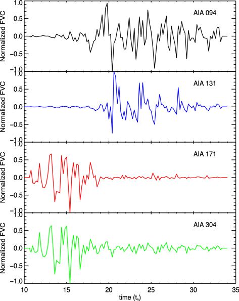

**Figure 12.** Normalized FVC of the AIA 94, 131, 171 and 304 Å channels in the turbulent region above the loop-top from t = 10t_A to t = 35t_A.
Download figure:
Standard image High-resolution image

Table 1. Summary of the Period of QPPs in Different Wavelengths

Wavelength	Period of QPPs		Period in Physical Time
SDO/AIA 94 Å	1.39t_A	2.34t_A	67.18 s	113.09 s
SDO/AIA 131 Å	1.65t_A	2.78t_A	79.74 s	134.36 s
SDO/AIA 171 Å	1.65t_A		79.74 s
SDO/AIA 304 Å	1.65t_A		79.74 s

Download table as: ASCII Typeset image

4. Summary and Discussion

The study of the plasma heating process via turbulence is important for explaining the complex thermal structure of hot plasmas observed in eruptive solar flares. In this work, we performed the 2.5D MHD simulations based on the CSHKP model with a gravitationally stratified solar atmosphere, high Lundquist number (S = 10⁶), anisotropic thermal conduction and radiative cooling included. We focus on the properties of turbulence at different locations (inside the CS or above the flare loops) in the steady reconnection phase and the associated temperature distribution. We find that the temperature distribution of the CS is not symmetric with respect to the principal X-point, and the conductive losses and radiative losses compete in different reconnection phases. In particular, when the growing speed of the reconnection outflow exceeds the local magnetosonic speed at the loop-top, a TS is formed thereby (Shen et al. 2018). As the turbulence develops, multiple TSs interact and combine with each other, which cause the change of the spectrum index and eventually heats the plasma at the loop-top. Since empirical cooling mechanisms are considered, we are allowed to make the forward modeling of the EUV emission from the simulated profiles. The variety of morphologies with respect to turbulence are displayed in different SDO/AIA passbands. This provides a straightforward way to access the finer thermal structures of the CS in comparison with spectroscopic observations and a reliable prediction of light curves in the SAF. Our main results are summarized as follows.

(1)
The thermal structures of the fragmented CS and the flare loops are exhaustively studied by high-resolution MHD simulation. The use of the semi-implicit solver for thermal conduction as described in Ye et al. (2019a) consequently realized an acceleration of ∼300 in terms of the computation efficiency. Since the gravitationally stratified atmosphere is used, the upward CS can be heated to a higher temperature than the downward part, which is consistent with the simulation work of solar eruptions by Reeves et al. (2010). It also can be seen that the downward reconnection jets heat the chromosphere plasma causing it to rise and fill the loops in this model. We observe that the temperature of the CS and the flare loops is smoothly distributed, undergoing the impulsive and decay phases in general. The density cavity above the postflare loops could be responsible for the dimming region found in multiwavelength observations. The reconnection rate obtained is similar to the work of Shen et al. (2011), in which thermal conduction and radiative cooling are neglected. As plasmoid instability begins to develop at about t = 16t_A, the rate rises rapidly from 0.01 to 0.1 and stabilizes afterwards.
(2)
Regarding the energy transport in a fixed box covering the CS and the coronal flare, conductive and radiative losses play a nonnegligible role in determining the structures of hot plasmas. The calculation is initialized from the thermal equilibrium condition, and radiative losses dominate for the major evolution time. As the loop and the CS becomes hotter, conductive losses are found to be comparable with radiative losses in the later phase.
(3)
In the steady reconnection phase, the MHD turbulence inside the CS is shown to be anisotropic while that above the flare loops remains quasi-isotropic. By following two plasmoids successively merging to the flare loops, we observe that the magnetic spectrum becomes softer when they are interacting with the TSs. The passage of plasmoids can fracture the geometry of the TS into multiple segments and then fragmented CSs appear, which make the region above the flare loops more turbulent to allow for quickening of the energy dissipation. One can find that the loop-top is heated by TSs, and the turbulence induced by plasmoids can make the plasmas thereby heated to a higher temperature, which could be responsible for the intermittent nature of the SXR and HXR observed by RHESSI.
(4)
The forward modeling of the EUV emission from the simulated data clearly shows the radiation enhancement by turbulence in the AIA 94, 131 Å channels, while it is not significant in the other channels (AIA 173, 304, 193 Å). The spectrum study of the radiation intensity in these wavelengths gives quite different power indices at the same time, of which the ones for AIA 131, 193 Å are greatly consistent with the observation by Cheng et al. (2018). The calculation for the synthetic Fe xxi 1354.08 Å line reveals that the Doppler width is larger at the location of plasmoids than the other places in the CS. In addition, we have also shown the corresponding light curves in the turbulent region above the loop-top in flare phases to compare with the SAF observations by Cai et al. (2019). By using the Morlet wavelet transform, the dominant periods of the plasmoid generation rate, the transverse oscillation above the loop-top, and QPPs in the SAF are calculated. As a result, the high-temperature passbands (AIA 94, 131 Å) both have two dominant periods responsible for the intermittent heating via reconnection outflows and plasmoid collisions, while the low-temperature passbands (AIA 171 and 304 Å) have an identical period responsible for the change in density of the SAF. The kink-mode oscillations might be related to density perturbations in QPPs, but the heating for plasmas via turbulence is an important contributor to the source of QPPs in the SAF as well.

Our results also imply that the multiple TSs and turbulence could be the accelerators for loop-top nonthermal particles. The value of the divergence of the velocity field in Figure 4(b) identifies the locations of strong compression, an indication of multiple shock fronts. The first-order Fermi acceleration can take place efficiently at multiple TSs (Mann et al. 2006, 2009; Chen et al. 2015). Another possibility is that the second-order Fermi acceleration induced by stochastic process (Petrosian & Liu 2004; Fang et al. 2016) and the efficiency of the acceleration in turbulence strongly depend on the short-wavelength structures (or high-wavenumber components). As interpreted in Figure 6(b), the smaller-scale structures at the loop-top are constantly generated due to multiple TS mergers and plasmoid collisions. Thus, stochastic acceleration via turbulence could play an important role in this region as well. On the other hand, as suggested by Drake et al. (2019), fragmented current layers consist of multiple magnetic islands, which might be an efficient driver of energetic particles via the first-order Fermi acceleration in flare observations. The forward and inverse coalescence of plasmoids generates small-scale reconnecting X-lines when the turbulent spectral indices vary around −2 as in Figure 5. Particles reflect from the moving field lines and gain energy over broad regions of the CS.

In general, the thermal structures simulated in our work are strongly in agreement with observation results. We are allowed to have access to the small-scale structures in the large-scale background of the flaring process and give a prediction of morphologies of the MHD turbulence in EUV emissions or light curves for the specified locations. This can also provide the necessary information for detecting the TS in multiple-wavelength observations. However, since the Kelvin–Helmholtz instability is a possible ingredient for loop-top turbulence (Fang et al. 2016), the realistic heating function and chromospheric evaporation will be considered in future work. Furthermore, our findings in this paper need to be reinvestigated and confirmed in large-scale 3D simulations because of more complicated 3D turbulent structures found in the reconnection outflow region (Daughton et al. 2011; Guo et al. 2015; Huang & Bhattacharjee 2016).

The authors would like to thank the anonymous referee for the valuable and constructive comments and suggestions that helped improve this work significantly. This work was supported by the Strategic Priority Research Program of CAS with grant XDA17040507; NSFC grants 11603070, 11933009; CAS grants QYZDJ-SSWSLH012 and XDA15010900; and the grant associated with the project of the Group for Innovation of Yunnan Province 2018HC023, the Yunnan Province Yunling Scholar Project. CHIANTI is a collaborative project involving George Mason University, the University of Michigan (USA) and the University of Cambridge (UK). The work was carried out at the National Supercomputer Center in Tianjin, and the calculations were performed on the Tianhe 3 prototype.

Software: Athena 4.2.

The Role of Turbulence for Heating Plasmas in Eruptive Solar Flares

Article metrics

Permissions

Author affiliations

ORCID iDs

Dates

Abstract

1. Introduction