


Abstract
The role of ideal-MHD instabilities in a prominence eruption is explored through 2D and 3D kinematic analysis of an event observed with the Solar Dynamics Observatory and the Solar Terrestrial Relations Observatory between 22:06 UT on 2013 February 26 and 04:06 UT on 2013 February 27. A series of 3D radial slits are used to extract height–time profiles ranging from the midpoint of the prominence leading edge to the southeastern footpoint. These height–time profiles are fit with a kinematic model combining linear and nonlinear rise phases, returning the nonlinear onset time (tnl) as a free parameter. A range (1.5–4.0) of temporal power indices (i.e., β in the nonlinear term ) are considered to prevent prescribing any particular form of nonlinear kinematics. The decay index experienced by the leading edge is explored using a radial profile of the transverse magnetic field from a PFSS extrapolation above the prominence region. Critical decay indices are extracted for each slit at their own specific values of height at the nonlinear phase onset (h(tnl)) and filtered to focus on instances resulting from kinematic fits with (restricting β to 1.9–3.9). Based on this measure of the critical decay index along the prominence structure, we find strong evidence that the torus instability is the mechanism driving this prominence eruption. Defining any single decay index as being "critical" is not that critical because there is no single canonical or critical value of decay index through which all eruptions must succeed.


Original content from this work may be used under the terms of the Creative Commons Attribution 4.0 licence. Any further distribution of this work must maintain attribution to the author(s) and the title of the work, journal citation and DOI.
1. Introduction
Solar prominences commonly appear as cool, dense, and elongated features suspended in the lower solar atmosphere (Engvold 2015, and references therein). At 103–104 K they are significantly colder than the MK corona they are suspended within. As a result, they appear in absorption when contrasted against the solar disk and in emission in certain wavelengths when contrasted against space at the limb. On-disk they are known as filaments; however, hereafter we refer to disk and limb structures simply as prominences. While prominences mostly exist at latitudes between ±60°, the majority of the longest were found between ±(30°–60°) (Wang et al. 2010). The length of a prominence will usually be found in the range of 30–110 Mm (Bernasconi et al. 2005). Wang et al. (2010) also find an average height of 26 Mm for prominences, though it should be noted that quiescent prominences can reach much greater heights (Loboda & Bogachev 2015), with one example reaching 150 Mm. Many properties of a prominence depend on its magnetic environment. Those found in active regions (ARs) are smaller, shorter-lived, and much lower in height than those found in quiet-Sun (QS) regions (Parenti 2014). Regardless of whether they are found in ARs or QS regions, prominences lie between photospheric magnetic fields of opposing polarity, along the polarity inversion line (PIL).
Prominences are considered to exist within one of two magnetic configurations—sheared arcades (Antiochos et al. 1994) or stable magnetic flux ropes (MFRs; Kuperus & Raadu 1974). In either case, the mass of the prominence settles within the structure from the overlying corona to fill "dips" in the magnetic structure (Gibson 2018). In the case of sheared arcades, plasma accumulates near the apices of the sheared loops. In the flux rope model, the mass collects in the "dips" of the poloidal field. In both models the dips form a continuous stream of plasma through the structure, which is then observed as the prominence. However, Aulanier & Demoulin (1998) only considered a flux rope, and they noted that there is no guarantee that the mass fill the dips. The two models cannot be entirely separated, as sheared arcades can form MFRs as part of an eruptive process, though it is the onset of instability in MFRs that provides one preferential aspect in favor of the stable MFR model. The evolution of an MFR, whether preexisting or newly formed, is highly dependent on its relation to the background magnetic field, as will be discussed in the following text.
1.1. Eruption Instabilities
For MFRs, eruptive mechanisms invoke these structures reaching some criteria of instability. These criteria can be separated into ideal processes, e.g., the kink instability (KI; Török & Kliem 2005) and torus instability (TI; Kliem & Török 2006) that will be discussed in detail later, or resistive processes, e.g., tether-cutting (Moore et al. 2001) and breakout reconnection (Antiochos 1998).
In all cases, however, the magnetic field plays an extremely important role in governing the onset and development of the eruption. Specifically, gradients in the magnetic field play a key role in whether an eruption will "succeed," i.e., whether the eruption will eject material into space. In some cases, such as Török & Kliem (2005), the eruptive mechanism cannot overcome the overlying magnetic field and the eruption will result in a "failed" or "partial" eruption. This is especially important when considering the TI, as that mechanism is directly related to the magnetic field gradient, as will be discussed further later.
1.1.1. Kink Instability
The KI was first suggested as an eruptive mechanism by Sakurai (1976) but has taken on a greater role in the explanation of both confined and fully eruptive events since it was shown to be feasible for both by Török & Kliem (2005) and references therein.
Perhaps the most obvious observation of the KI is presented in Török & Kliem (2005). This AR filament eruption displayed two important properties of the KI. The first is that the instability can lead to reconnection under sufficient confinement. The second is that the confinement of the flux rope is dependent on the overlying field. In an AR, the overlying field gradient typically decreases much more slowly than the field overlying quiescent regions. This confinement is a major contributor to whether the instability will reach saturation or whether other processes, such as the TI, will begin to act on the flux rope.
1.1.2. Torus Instability
The TI is best thought of as a loss of equilibrium between a radially outward force and a radially inward force. This force balance was originally described by Shafranov (1966), who considered it as a toroidal Lorentz force combined with the net pressure gradient of a curved current channel balanced by the transverse component of an external poloidal magnetic field, Bex, also generated by a Lorentz force. A potential cause for a loss of equilibrium was considered by Bateman (1978), who found that a torus would expand, after perturbation, against an external poloidal field that decreased by at least a critical rate in the direction of the major radius, R. This dimensionless rate is called the decay index, n, and was derived by Bateman as

with a critical value at ncrit > 1.5 when an overlying field of is assumed. This condition is based on the toroidal Lorentz force decreasing with the expansion of the torus, but decreasing at a lower rate than the external magnetic field. This effect was demonstrated in an experimental approximation of a prominence by Hansen & Bellan (2001), who showed the balancing ability of an external "strapping" force.

Kliem & Török (2006) analyzed the instability in regard to coronal mass ejections (CMEs) for the large aspect-ratio regime and with the simplification of only considering the stabilizing external field and the toroidal Lorentz force. They found that it was possible for the TI to be the driving mechanism of a CME and would likely guide its evolution. They tested several decay indices and noted a difference in the resulting acceleration profiles. This was later used (Török & Kliem 2007) to show that the resultant CME's velocity profile would be affected by the gradient of the overlying field.
Given the importance of the critical value of the decay index, much work has been dedicated to confining the range of values it could take. Table 1 presents measurements of the critical value, derived from both observations and simulations for events within both active and quiet-Sun environments, across a range of studies. Here we group critical values based on the location where it is determined. As can be seen in Table 1, the critical value is generally found to be lower when measured at the top of the prominence mass than at the location of the flux rope axis. This has been confirmed numerically by Zuccarello et al. (2016), who show that where the critical decay index is measured within the same event can lead to very different results, and is likely to be the reason for the apparent difference between theoretical and observational results. They show that changing the point of calculation from the flux rope's axis to the estimated top of the prominence mass changed from ncrit ≈ 1.4 ± 0.1 to ncrit ≈ 1.1 ± 0.1. In general, the differences between studies result from differing model setups and the choice of which event is considered. For example, Démoulin & Aulanier (2010) show the importance of the shape of the flux rope and its properties in determining the critical value of the decay index.
Table 1. Decay Index Values
| Vertical Location through Prominence/FR | Critical | Study | Source | References |
|---|---|---|---|---|
| Structure | Decay Index | Type | Region | |
| Prominence mass | 1.74, 2.04a | Obs. | AR | Liu (2008) |
| Prominence mass | >2.5b | Obs. | AR | Liu et al. (2010) |
| Prominence mass | 0.98–1.68c | Obs. | QS | Xu et al. (2012) |
| Prominence mass | ≥1 | Obs. | AR | Zuccarello et al. (2014a, 2014b) |
| Prominence mass | 1.20 ± 0.29d | Obs. | QS | McCauley et al. (2015) |
| Prominence mass | 0.9–1.1 | Obs. | AR | Lee et al. (2016) |
| Prominence mass (magnetic dips below FR axis) | 1.1 ± 0.1 | Sim. | AR | Zuccarello et al. (2016) |
| Prominence mass | 0–2e | Obs. | QS | Aggarwal et al. (2018) |
| Prominence mass | 1.2 ± 0.1 | Obs. | QS | Sarkar et al. (2019) |
| Prominence mass | 0.8–1.3 | Obs. | AR | Vasantharaju et al. (2019) |
| FR axis | ≥1.5 | Ana. | ... | Bateman (1978) |
| FR axis | ≈1.5 | Ana. | QS | Kliem & Török (2006) |
| FR axis | >1.5 | Ana. | AR | Kliem & Török (2006) |
| FR axis | ∼2 | Sim. | QS | Fan & Gibson (2007) |
| FR axis (location of thin current channel) | 1.1f, 1.3g | Sim. | AR | Démoulin & Aulanier (2010) |
| FR axis | 1.5–1.75 | Sim. | AR | Kliem et al. (2013) |
| FR axis | Obs. | AR | Jiang et al. (2016) | |
| FR axis | 1.4 ± 0.1 | Sim. | AR | Zuccarello et al. (2016) |
| FR axis (highest-lying NLFFF lines over PIL) | >0.8h | Obs. | AR | Jing et al. (2018) |
| FR axis (cavity centroid) | 1.3 ± 0.1 | Obs. | QS | Sarkar et al. (2019) |

Notes.
aAveraged over 42–105 Mm. bAveraged over 42–105 Mm. cFor the five QS events averaged over 42–105 Mm. dSee Table 5 in reference. eMany events, each averaged over 42–105 Mm. See Figure 5(e) in reference. fFor straight current channels. gFor curved current channels. hIn the sample studied, all events showing decay indices >0.8 were ejective (i.e., all of the confined events had <0.8), although ejective events did span this threshold.Download table as: ASCIITypeset image
We will now consider the observational signatures of the KI and TI, respectively.
1.2. Observational Signatures
KI.—The most clear signature of the KI is the evolution of the shape of the prominence as it writhes. However, the writhe that causes this change in shape can also develop from shear-field-driven writhing, reconnection with the surrounding field, or the straightening of the sigmoid. Kliem et al. (2012) state that unambiguous signatures of the KI would be flux rope legs approaching each other, an apex rotation of over 130°, and multiple helical turns developing over the structure. However, the level to which these are visible is dependent on how far the instability develops, which itself is dependent on the confinement of the structure. For an unconfined event we should not necessarily expect to see total saturation. We should instead expect to see the structure show the development of writhe as it evolves, while at the same time being able to rule out the other sources of writhe. Accurate calculation of the writhe will require careful determination of the 3D structure.
TI.—An important feature of the TI is its dependence on the height of a critical decay index being reached by the MFR for the eruption to begin. As the MFR may not be observed, we instead consider the prominence-mass leading edge. A slowly varying decay index should, in principle, allow us to rule out breakout and tether-cutting (nonideal) eruption scenarios, which would otherwise lead to more abrupt decay index variation and potentially only impacting on part of the structure. As a result of this, one must be very careful about using a single critical value to define an event because the derived critical decay index may only be valid for a small section of the structure. Therefore, the decay index should be evaluated along a significant portion of the structure. In addition, it should not be inferred that the observed height of the prominence leading edge at the time of eruption is necessarily the height at which the eruption has begun. This is due to the previously mentioned difference between the position of the prominence mass and the flux rope axis.
In Section 2 we overview the observations of a quiet-Sun prominence eruption, for which we will conduct a detailed 2D and 3D kinematics study of the prominence leading edge, in order to identify the onset of acceleration in the eruption and observational signatures of the governing eruption instability. In Section 3 we outline two contrasting methodologies for determination of the prominence leading edge height as a function of time. The first method (Section 3.1) automates the detection of the leading edge for determination of 2D plane-of-sky heights and is optimal for high-cadence (12 s) Solar Dynamics Observatory (SDO) observations. The second method (Section 3.2) applies a nonautomated stereoscopic approach for determination of 3D heights along the prominence structure but limited by the low-cadence (600 s) STEREO-A observations. In Section 3.2.2 we conduct a piecewise kinematic profile fitting of the height–time data for 137 locations along the prominence leading edge to extract important eruption properties such as time of onset of the nonlinear phase, height at time of onset, and onset starting height, as well as kinematic properties of linear velocity and acceleration of the eruption for a range of power indices. In Section 3.3 we investigate the PFSS magnetic field model for the event to determine the critical decay index. We compare the critical height derived from the magnetic field extrapolations with the height at time of onset derived from observations for each of the 137 locations, revealing remarkable results on the nature of the eruption mechanism. In Section 4, these results are discussed and conclusions are drawn.
2. Observations
The focus of this study is a "quiet-Sun" prominence that erupted from a location close to the solar west limb over 2013 February 26–27 and resulted in a CME.3 The primary data used in this work are images from the 304 Å channels of both the Atmospheric Imaging Assembly (AIA; Lemen et al. 2012) on board the SDO (Pesnell et al. 2012) and the Extreme Ultraviolet Imager (EUVI; Wuelser et al. 2004) on board the Solar Terrestrial Relation Observatory (STEREO; Kaiser et al. 2008), specifically the Ahead (A) spacecraft.
As Figure 1 depicts, STEREO-A was located 131° in longitude ahead of the Earth-orbiting SDO spacecraft when the prominence eruption occurred. The degree of satellite separation and the location of the prominence (almost midway between them) enable the determination of 3D coordinates by stereoscopy. This is illustrated in Figure 2, where a point on the SDO-viewed prominence is selected (left panel, blue triangle) and its 3D line of sight is projected onto the STEREO-A plane of sky (right panel, dotted line). Human interaction is then required to select which point along that line of sight is most likely to be the same feature (right panel, blue triangle), resulting in a two-viewpoint triangulation of 3D coordinates. These coordinates are then used to define a series of 3D radial "slits" that are projected onto the AIA plane of sky (left panel, straight white lines) for the Section 3.1 initial 2D analysis. Note that Section 3.2 contains a more complete description of the application of these stereoscopic analysis techniques for the 3D reconstruction of the prominence leading edge (Figure 2, left and right panels, green curves).

Figure 1. Relative positions of SDO (orbiting Earth) and STEREO-A at the time of the prominence eruption.
Download figure:
Standard image High-resolution image
Figure 2. Cotemporal SDO/AIA 304 Å and STEREO-A/EUVI 304 Å intensity images of the prominence.
Download figure:
Standard image High-resolution imageThe eruption occurs slowly and with no visible brightening in AIA or EUVI-A or in any X-ray channels. This suggests no presence of particle-acceleration-related brightenings (e.g., tether-cutting; Moore et al. 2001), and thus we suggest that reconnection was not a driving force behind this eruption.
3. Methods and Results
3.1. AIA Data Analysis
We have developed a novel, automated, edge detection procedure to determine the location of the prominence edge applied to the height–time profiles from each of the 137 radial slits as shown in Figure 2. This is a more rigorous approach in measuring the location of the edge (incorporating a height error on all detected edge pixels) and its variation in time, compared with standard thresholding techniques commonly adopted for prominence edge detection studies. This procedure is carried out in four stages.
Stage I. The background, shown as a dashed blue line in Figure 3, is calculated as the mean+6σ of the pixel intensities taken from the upper left corner of the height–time plot from the southernmost slit (the boxed area within Figure 4), where σ is the standard deviation of the intensities within that area. We use the southernmost slit because this is where there is the greatest separation between limb and detector edge. This background value was then applied as the threshold to all slits with any pixel found below this value set to zero.

Figure 3. Position of the detected edges for an individual time slice. As in the height–time plots, the green line corresponds to the derivative threshold line, the blue line to the background line, and the yellow line to their average. The inset is the derivative of the intensity profile along that slit, with the gray dashed lines showing the search range around the background-detected pixel.
Download figure:
Standard image High-resolution image
Figure 4. In all height–time plots, the green line is the derivative threshold, the blue line is the background threshold, the yellow line is the average of the derivative and background thresholds, and the white line fit to the edge is the boxcar-smoothed height line. The left y-axis shows the height measured from the 3D position at which R⊙ = 1. The right y-axis shows the height measured from the plane-of-sky height at which R⊙ = 1. The dashed white lines show the extent of the background area within this smaller FOV. In the bottom three panels we show an example of a leading edge discontinuity (i.e., "dropout") from each slit.
Download figure:
Standard image High-resolution imageStage II. We then apply a transient feature filter to the remaining height–time intensity plot for each slit. The overall effect of the filtering is that any nonzero pixel that is not spatially and temporally related to the main body of the prominence is put to zero. However, transient features that are connected to the main body of the prominence, at some point in time, are preserved (i.e., not zeroed) as potential deviations of the prominence leading edge. A detailed description of this process is provided in Appendix A.
Stage III. In each time slice, the greatest height of any nonzero pixel becomes the upper detection boundary as can be seen as the short solid vertical blue line in Figure 3. We then search for the maximum negative intensity derivative in the outward direction within the same time slice. To avoid detecting lower-lying edges below the main prominence, the derivative search is restricted to a height range of ±∼10 Mm (15 6 or 26 pixels) from the background-detected edge. This is represented in Figure 3 by the solid vertical green line, which becomes the lower detection boundary. The prominence edge is then defined as the average height of the background- and derivative-detected boundaries, shown as the solid vertical yellow line in Figure 3. An uncertainty is assigned as half the difference between these boundaries, with a minimum of 1 pixel (i.e., when they identify the same pixel).
Stage IV. After the prominence edge has been detected in all time slices, a running boxcar approach is applied using a user-defined boxcar width. Edge heights in the boxcar sections are linearly fit using the IDL routine MPFIT to calculate their average radial velocities. This routine uses the Levenberg–Marquardt method to solve the least-squares problem.
Following these four stages, the detection of the prominence edge is overlaid onto the height–time intensity plots, as shown in Figure 4 for slits 0, 68, and 136. The method performs extremely well, providing a consistent edge in time. An example of this consistency is found between 01:06 UT and 02:36 UT in slit 0, where there exist gaps in the prominence beneath the detected edge. However, there can exist spurious dropouts in structures at the leading edge over short intervals of time, for example, at ∼03:20 UT in slit 68, highlighted in the bottom middle panel, which will have an impact on accurate determination of kinematics at such time intervals. When comparing all three height–time profiles, it is clear that the onset of the eruption appears to evolve earlier in lower slit numbers (i.e., closer to the center of the prominence's 3D loop structure).
Figures 5(a) (side-on view) and (b) (top-down view) show the leading edge height–time profiles for all 137 slits, stacked together and color-coded by their running boxcar linear velocities (determined after fitting the height–time sections following Stage IV). When comparing all slits, the maximum outward velocity is 48.6 km s−1. All slits reach at least 30 km s−1. Figure 5(c) shows the running boxcar linear velocity profiles averaged across all slits, highlighting a slow, nearly linear rise phase of <5 km s−1 prior to acceleration in the eruption. It is important to remember that the slits shown here diverge with height, which can explain the existence of features in the surface plots that cease to exist in neighboring slits. As mentioned, the height–time profiles and the corresponding velocity profiles are marred by plasma dropouts that are distinctive in the velocity color profiling of Figures 5(a) and (b). These manifest as dark streaks followed shortly afterward by bright streaks characterizing a sudden dip in the leading edge, e.g., between 00:36 UT and 01:36 UT for slits 50–70. Some plasma dropouts span many slits, for instance, the dark streak starting around 22:06 UT and lasting ∼15 minutes in slits 0–30 and appearing progressively later in slits 30–80. It is clear that velocity profiles in all slits depict some form of acceleration, with the onset tending toward later times for increasing slit numbers, i.e., the onset of eruption starting nearer the center of the prominence structure and progressively later farther along the edge. In part, this may be due to a notable plasma dropout masking the beginning of the acceleration phase, in particular with regard to slits 45–90 between 02:51 UT and 03:21 UT.

Figure 5. (a) Side-on view of the surface plot of height for each slit number vs. time. (b) Top-down view of the same surface plot. In both, color represents running boxcar linear velocity. (c) Running boxcar linear velocity averaged across all slits, with the green lines representing the standard deviation of the velocity across all slits.
Download figure:
Standard image High-resolution imageThe leading edge is clearly dynamic while the eruption ensues, and a physical explanation on the nature of the dropouts is not investigated here. The purpose of this research is to accurately determine the onset time of acceleration in the eruption, and it is clear that the plasma dropouts inject a strong influence on many height–time profiles. This prevents an accurate, effective interpretation of the transitions in velocity (and more so acceleration) at critical times prior to the onset of acceleration in the eruption. The running boxcar linear velocity study provides a qualitative interpretation of the evolution of the leading edge prior to and during the eruption. To reach a quantitative assessment of this transition to acceleration, we apply a more interpretable forward fitting approach. This will take the form of a parametric study into the onset time of acceleration through examination of a two-component fit (consisting of linear and nonlinear terms) to all slit profiles. The details will be further discussed in Section 3.2.2. A two-component forward fitting approach will be performed on the lower-cadence stereoscopic results. This will allow the kinematic study of the eruption to be applied directly on the 3D-determined stereoscopic height–time profiles, which are a truer determination of heights in the eruption. Lower-cadence observations also provide added value of suppressing the impact of the dropouts in the time series. The running boxcar linear velocity results will be placed in context with this alternative forward fitting approach.
3.2. Stereoscopic Data Analysis
The prominence was observed in the He ii 304 Å passband by both SDO/AIA and STEREO/EUVI-A, with a separation angle of 131°, as shown in Figure 1, enabling 3D reconstructions of the leading edge. To construct 3D loops characterizing the prominence leading edge, we use the SSWIDL widget scc_measure.pro for coincident pairs of AIA and EUVI-A images, throughout the eruption. In order to identify a 3D coordinate along the prominence leading edge, the user first selects a pixel on one image (either AIA or EUVI-A). We first select a pixel location from the AIA image because from that perspective the prominence edge is most clearly defined by eye at the limb (blue triangle in Figure 6, first column). The software then displays a near-horizontal dashed white line on the corresponding EUVI-A image (Figure 6 second column), i.e., this line represents the 3D line of sight of a selected SDO image-plane pixel and its deprojection into the STEREO-A image plane.

Figure 6. (a–e) Evolution of the prominence undergoing eruption, in hourly time steps. First column: the prominence as observed at 304 Å with SDO/AIA. The solid green line indicates the 3D reconstructed prominence leading edge deprojected onto the FOV. The blue symbol marks the maximum height pixel for the detected edge. The solid white line is the radial slit 0. Second column: coincident images of the prominence eruption as observed at 304 Å with STEREO/EUVI-A. The solid green line indicates the 3D reconstructed prominence leading edge deprojected onto the FOV. The solid yellow lines are the northernmost and southernmost 3D reconstructions of the prominence structure. The dashed white line represents the line of sight with respect to the maximum height pixel from the AIA image as it appears deprojected into the EUVI-A plane of sky. Third and fourth columns: top-down (i.e., aerial) and side-on perspectives, respectively, of the 3D prominence leading edge incorporating the solid green/yellow line reconstructions, visualized in 3D with VAPOR (https://www.vapor.ucar.edu). The maximum height location is again marked with a blue symbol. The axes of these 3D visualizations represent latitude and longitude in the Heliographic/Stonyhurst coordinate system and radial height in units of R⊙.
Download figure:
Standard image High-resolution imageWe then manually select an EUVI-A pixel lying along this line, which, by eye, defines a coordinate in 3D space (i.e., blue triangle in Figure 6, second column). The 3D coordinates of all selected locations along the edge in the first/second column image pairs in Figures 6(a)–(e) are then calculated and stored as (Earth-based) Stonyhurst heliographic longitude and latitude, along with radial distance. For each image pair this process was repeated for at least 50 AIA pixel locations, tracing the visible prominence edge as a loop within the AIA image (solid green line in Figure 6, first column).
Each location along the loop has a corresponding location in EUVI-A (solid green line in Figure 6, second column), resulting in a 3D loop coordinate set. This process is repeated for all matching AIA and EUVI-A image pairs throughout the observation. (Note that the total number of coincident image pairs in the full time series is only 36 given the EUVI-A cadence.) As the eruption progresses with height above the limb, the overall loop length will continually increase, resulting in a larger number of selected 3D coordinates (up to 140 at later times). An interpolation was applied to the 3D coordinate set for each loop to create an equal number of loop data points for all images in the sequence.
The blue triangle location in the first and second columns of Figure 6 represents the maximum height location of the 3D loop as it evolves in time for each panel row. With respect to slit 0 in Figure 6, in the AIA field of view (FOV), the maximum height location shifts northward in time, i.e., the loop apex shifts toward the geometric midpoint of the 3D loop structure, implying a distortion of the prominence leading edge as the eruption ensues. This distortion of the loop structure is clearly seen in the fourth column of Figure 6, where the reconstructed loops and maximum height locations are visualized in 3D from a side-on view. From a top-down view (third column) there appears to be very little evidence for distortion or even writhing of the reconstructed loops that one may expect if the KI were taking effect.
Finally, this loop reconstruction process was repeated twice, resulting in three independent measurements of the prominence structure, which can be identified as solid yellow curves above and below the solid green curve in the second column of Figure 6 and yellow lines bounding the green loop as visualized in the third and fourth columns of Figure 6. This was done because there is an uncertainty with regard to the choice of the matching 3D coordinate pixel along the dashed white line in the EUVI-A image frame. The narrow prominence channel cross section, visible on-disk in absorption within the EUVI-A image, intersects with the dashed white line for a number of pixels in its cross section. Any pixel along the line intersecting the channel could potentially represent the true location of the leading edge. To address this uncertainty, we consistently (by eye) selected the easternmost, center, and westernmost locations of the prominence channel with each repeated reconstruction. We still expect a resulting uncertainty in radial height of ∼2.8 Mm (i.e., ±1.4 Mm), given that the variation in 3D radial height between these three determinations of prominence spine location is ∼0.004 solar radii. This is the first step in the process of determining an eruption height–time profile, stereoscopically.
Clearly, the manual procedure in reconstructing the 3D leading edge is vulnerable to human judgment given that the choice of AIA pixel defining the edge is performed by eye in a point-and-click manner. We address this important issue with a correction to the radial height coordinates along the reconstructed loops. An intensity threshold is applied to the radial slit data deprojected onto the AIA FOV, with respect to each 3D coordinate, in order to establish a measure of uncertainty in the radial height measurement at the leading edge. This correction will be outlined in more detail in the next section.
3.2.1. 3D Height–Time Reconstruction
To establish height–time profiles characterizing the eruption, the same 137 radial slits applied in Section 3.1 (via the first method) are now used to intersect the 3D loop coordinates deprojected onto the AIA FOV. In order to accurately assess the kinematics of the prominence leading edge, we must evaluate the uncertainty in radial height measurement. It is important to note that the height measurement from 3D reconstruction will be preserved throughout this study and only the uncertainty on this height will be recovered after projection onto the AIA 2D plane, to be outlined next.
Figures 7(a)–(c) present intensity profiles and corresponding height–time profiles for slits 0, 68, and 136, respectively (previously displayed in Figure 4 via the first method). For each radial intensity profile, a 144'' section centered on the point-and-click pixel location (blue symbol) of the leading edge is used to search for the first detected background-level pixel (rightmost orange symbol), with respect to the outward radial direction, and the first detected 7σ-above-background pixel (leftmost orange symbol), with respect to the inward radial direction. The background-level intensity is the averaged intensity from a region of the AIA image that is far off-limb, free of activity, relatively close to the outermost path of the slits. The uncertainty in the height of the point-and-click pixel location was then established as the maximum range in height with respect to the background and 7σ pixel heights. These height uncertainties for the intensity profiles in Figures 7(a)–(c) are presented as horizontal blue error bars spanning a range of heights in arcseconds. In each panel, the intensity profiles correspond to a time interval in the associated height–time profiles (displayed below), indicated by open blue diamonds enclosing the height uncertainty now converted to units of solar radii. In Figure 7(b) (slit 68), we present an example of a very tightly bound height uncertainty where the point-and-click edge location was very accurate relative to the expected edge location, as defined by the last 7σ-above-background pixel location along the slit. In contrast, Figure 7(c) (slit 136) provides an example of where the point-and-click pixel appears to match an inner edge of the prominence structure, whereas the threshold-determined pixels are farther along the slit and possibly attributable to the outer edge of a transient feature above the prominence. The uncertainty in height within the height–time profile for slit 136 at this time is clearly substantially larger (bounded by the blue open diamond) than in neighboring time frames, making it likely to be a transient feature above the prominence.

Figure 7. (a–c) The 304 Å AIA intensity profiles for 3D radial slits 0, 68, and 136, respectively, deprojected onto the AIA FOV using the world coordinate system. The point-and-click detected edge of the prominence is indicated with the blue symbol. The first detected background-level pixel (rightmost orange symbol) and the first detected 7σ-above-background pixel (leftmost orange symbol) along the slit are indicated. The horizontal blue error bar represents a measure of the uncertainty in height of the detected edge. Each panel slit has an associated height–time profile plotted below. The intensity profile corresponds to a time interval in the height–time profiles indicated with the open blue diamond.
Download figure:
Standard image High-resolution imageFigure 4 highlighted gaps in the prominence beneath the detected edge (via the first method), in particular, between 01:06 UT and 02:36 UT for slit 0. In the height–time plot of Figure 7(a), we note that the height uncertainty for the same time interval for slit 0 is relatively large; therefore, the uncertainties take into account these potential transient features. Furthermore, in Figure 4 we observe an apparent trend toward a later onset time for acceleration in the eruption; this is again present in the 3D height–time profiles. More generally, when comparing both methods across other slits, there is clear agreement with regard to the locations of potentially ambiguous features at the prominence edge (from interpretation of the detected edge) from the first method and the locations of larger uncertainty via the second method that one would expect.
Next, we will investigate in more detail the onset time for acceleration in the eruption using a parametric fitting approach on the 3D height–time profiles and in a statistical manner. This will allow us to determine kinematic properties and variations along the length of the prominence leading edge that may reveal an underpinning eruption-instability-driving mechanism.
3.2.2. Parametric Fitting to 3D Height–Time Profiles
Using the IDL routine MPFITFUN (which performs the Levenberg–Marquardt technique on a user-supplied function), we parametrically fit all 137 3D height–time profiles of the prominence leading edge using a kinematic function of the form

Here h(t) is the returned height at time t, t is the number of seconds since start of observation (22:06:19 UT on 2013 February 26), h0 is the height at time t = 0, v0 is the linear velocity, tnl is the time of onset of the nonlinear or "acceleration" phase in the eruption, α is the acceleration-like multiplier, β is the acceleration-term power index, and is a Heaviside function that switches on at t = tnl. The complex interaction of these fit parameters led to fixing the acceleration-term power index β in order to have all of the other fit parameters unconstrained in value (i.e., h0, v0, α, and tnl). As a result, β was chosen to vary over the range of 1.5–4.0 in steps of 0.1, allowing for the full exploration of the parameter space indicated by various eruption models (see, e.g., Lynch et al. 2004; Schrijver et al. 2008, and references therein). This approach still allows the fitting process suitable freedom to find the start time of the acceleration phase, indicating the time by which the eruption instability has begun.4

Initial estimates for each free parameter are required by the fitting process, chosen here to be h0 = 120 Mm, v0 = 0.5 km s−1, α = 1 m s−β, and tnl = 15,000 s. Once the minimum χ2 has been found for a fit with a specific β, the four free parameters are output along with their formal 1σ errors calculated from the covariance matrix.
Figure 8(a) shows the components in the fitting function (red dotted, blue dashed, and solid green lines) that combine as the best fit to the observations (black symbols with error bars). It is important to note that the linear velocity component, v0t, continues to contribute to the model after the onset of the acceleration (i.e., t > tnl). Figures 8(b)–(g) display the 1σ extent of the best-fit models for a selection of β. For all best-fit parameter plots that follow in this section, a specific color is assigned to each β value from the IDL rainbow color table 39—i.e., black (β = 1.5) to purple (β = 1.8) to green (β = 2.9) to red (β = 4.0).

Figure 8. (a) Height–time profile of slit 68 overlaid with combinations of the best-fit model components. The horizontal dotted red line shows the starting height h0, the dashed blue line is the combined starting height h0 plus the linear velocity v0t term, while the solid green line is the combination of starting height plus linear velocity term plus the acceleration-like term. The green shaded box indicates the range of possible nonlinear phase onset times in this example. (b–g) Best-fit height–time models as central curves that are bounded above and below by curves indicating their 1σ extent (based on the returned best-fit parameter errors), with vertical lines marking the resultant nonlinear phase onset times colored according to the value of β.

Download figure:
Standard image High-resolution imageIn Figure 9, for all values of β we show overlays of the best-fit models to the individual height–time plots of slits 0, 68, and 136. Notably, over the full range of slit numbers the majority show best-fit results with a pattern similar to that of slit 68—higher values of β show earlier tnl onset times (i.e., the general color order of the vertical lines being red earliest to purple/black latest)—which is understandable based on the interplay between the model parameters β, tnl, and α. Higher values of β increase the curvature in the modeled height–time profile, which can be compensated for by decreasing the acceleration-like multiplier α in order to achieve a good fit. In turn, smaller values of α cause the point of visible departure from the linear component to appear later, which can be compensated by tnl moving earlier in the fitting. This is clearly demonstrated in Figures 8(c)–(g) with the shift of tnl (i.e., colored vertical lines) to earlier times for increasing β. Aside from the typical fit behavior exemplified by slit 68, in a small number of slits a greater degree of scatter is found in for β < 1.9 and β > 3.6. This is represented in Figure 9 by slits 0 and 136, but it is worth noting that the intermediate portion of the β parameter space still generally results in a smooth variation of earlier tnl with increasing β, e.g., between 02:56 and 03:26 for slit 0 and between 02:16 and 02:36 for slit 136. In regard to the more scattered tnl fit results found toward the extremities of β being considered, the of these fits will be considered in our interpretation of the results, to be discussed later. For completeness, the and results of the fits for h0, v0, and α, in regard to all slit numbers and β values, are presented and discussed in Appendix B.


Figure 9. Best-fit models for all values of β overlaid onto each height–time profile (represented as data points with vertical error bars) for slit 0 (top), slit 68 (middle), and slit 136 (bottom). Each model overlay is represented by a specific color assigned to each β value, i.e., purple (β = 1.5) to green (β = 2.7) to red (β = 4.0).
Download figure:
Standard image High-resolution imageIn Figure 10, we present the start times of the nonlinear phase tnl, as determined by the fitting process independently carried out for all slits, where each panel displays the results for a specific value of β (i.e., increasing left to right and top to bottom). It is clear that the fitting process fails to iterate away from the starting tnl estimate across the vast majority of slits for β ≤ 1.8. As stated previously and demonstrated here, there is a trend through β wherein the tnl found becomes earlier with increasing β for most slits. Notably, at the earliest time of acceleration (corresponding to slit 0), we find that the maximum height location of the 3D reconstructed loop coincides with the intersection of slit 0 (as shown in Figure 6, first row). This is expected given that the eruption should start at the apex of the prominence structure according to the TI, and furthermore, this result addresses the second observational signature relating to the TI (as mentioned in Section 1.2). Overall, with regard to , a general trend is observed whereby tnl consistently becomes later with increasing slit number, indicating the presence of an underlying, coherent, evolving physical process at play across slits.


Figure 10. Time of onset of the nonlinear ("acceleration") phase, tnl. Each panel displays the results for a specific value of β (i.e., increasing left to right and top to bottom) using the same color scheme as in previous figures.
Download figure:
Standard image High-resolution imageIn Figure 11, we present the height of the prominence at the time of acceleration, h(tnl), as determined for each slit from the best-fit parameters. These are not measurements of the height across the prominence structure at an instant in time; rather, these are heights corresponding to the time of acceleration in a given slit. As before, we do not consider the results for owing to their poor fits. When considering a single slit number (across all β), there is a general progression to lower with increasing β, which we expect given that we determine earlier tnl with increasing β. When considering a single value of β (across all slit numbers), we observe a slight trend of increasing with increasing slit number. As mentioned above, the use of slit-dependent tnl values means that this result cannot be interpreted simply as an increase in height along the prominence structure, but instead that slightly greater heights are achieved for larger slit numbers at the later tnl values recovered for those slits. Over all slits we find values for that are relatively consistent along the prominence structure, the implications of which will be discussed later.


Figure 11. Height at the time of onset of the nonlinear phase, h(tnl). Each panel displays the results for a specific value of β (i.e., increasing left to right and top to bottom) using the same color scheme as in previous figures.
Download figure:
Standard image High-resolution image3.3. Magnetic Field Decay Index
Now that we have established a relatively constant h(tnl) across adjacent slits, we will next explore the variability of the decay index for this event. We once again note that the slits diverge as they increase in height, causing the horizontal separation between measured points along the prominence edge to increase as the prominence increases in height.
In order to calculate the decay index using Equation (1), we make use of a potential magnetic field model from the SSWIDL package PFSS (Schrijver & De Rosa 2003). Ideally, we would like to use a PFSS field extrapolation resulting from the photospheric field closest to the time of eruption. However, given that the eruption occurs close to the Earth-viewed limb, we instead use a PFSS extrapolation from when the prominence was at disk center (i.e., 12:04 UT on 2013 February 21) as shown in Figures 12(a)–(c). Examining an extrapolation primarily based on disk-center magnetogram observations minimizes the impact of projection effects and ensures that there is no contribution from the flux transport model that the PFSS method transitions to when approaching the Earth-viewed limb (i.e., keeping the extrapolation as data constrained as possible).

Figure 12. (a) Prominence observed in 193 Å by SDO/AIA at 12:04 UT on 2013 February 21. (b) SDO/HMI magnetogram of the same region. (c) PFSS solution from the same time, with field lines drawn starting from the region bounded by the Carrington coordinates of longitude 0°–26° and latitude −46° to −20°. (d) Mean decay index vs. height over the observed height range. (e) Box and whisker plots showing the range of decay index values over β. Individual box and whisker plots are displayed for each slit, using the nonlinear phase onset times specifically found for that slit (at each β). Purple plots correspond to the results from all fits (hence all β values), while gold plots correspond to results from fits with . (f) Box and whisker plots of the range of filtered decay index values as snapshots across the structure at a sequence of specific times.

Download figure:
Standard image High-resolution imageIn Figure 12(a), we show the prominence in absorption at this time as observed in 193 Å by SDO/AIA. The axis of the prominence channel is clearly coincident with the location of the PIL that separates the opposite-polarity fields in the lower half of the native-resolution SDO/HMI magnetogram of Figure 12(b) and the corresponding closed fields of the PFSS extrapolation in Figure 12(c). From the observations, comparing Figure 12(a) with Figure 2 from STEREO-A, it appears that the prominence experiences no significant evolution from when it exists at disk center until later at the limb prior to eruption. Note that the input magnetogram into the PFSS calculation, as shown in Figure 12(c), is a smoothed and resampled version of that in Figure 12(b), which is at full SDO/HMI resolution. We also tested nonlinear and linear force-free extrapolations with these PFSS lower boundary magnetogram data. However, the solutions for both converged toward that of a potential field. Aside from a small degree of field connectivity with the northerly AR, we therefore assume that the large-scale field overlying the prominence PIL is dominated by potential fields.
Using the PFSS extrapolation, we calculate the transverse component of the field, Bt, at each height step as

where and Bθ are the longitudinal and latitudinal components of the magnetic field, respectively. This is assumed to be dominated by an external constraining field at higher altitudes (i.e., Bt ≈ Bex). In order to construct a relevant average decay index profile as a function of radial height for the prominence region studied here, we first differentially rotate the 3D latitude/longitude coordinates of where slits 0–136 intersect with the prominence leading edge back to the time of the PFSS solution. These locations are shown as a green solid curve overlaid in Figures 12(a) and (b). We then calculate the individual decay index profiles (i.e., n(h)) for each of these 1°-sampled leading edge intersection coordinates, before averaging them separately at each height step to achieve the mean decay index profile displayed in Figure 12(d). The vertical dashed lines indicate the upper and lower limits of h(tnl) for all slits (i.e., 140–190 Mm), as shown in Figure 11. A horizontal dotted line is placed at the canonical value of ncrit = 1.5. Notice that within these limits all slits indicate a decay index value above 1.5 at the time of nonlinear phase onset. This mean decay index profile at the known PFSS heights is then cubicly interpolated to the values (for each β in each slit) using the SSWIDL routine dspline. We further explored the effect of spatial averaging by considering the influence of averaging over increasing areas beyond the 1°-wide region mentioned above. However, none of the different formats of averaging affect the decay index profile in the height range that we are interested in (i.e., h ≥ 140 Mm) by more than 2%. It is worth noting that the section of the prominence structure that we sample only spans the midportion of the structure that is well within the lateral extent of the opposite-polarity flux concentrations and is therefore not close to the MFR legs, so large variations in the background field decay index are not expected.


In Figure 12(e), we present box and whisker diagrams for each slit that characterize the derived decay index range for h(tnl) across β. Each box and whisker plot displays the characteristics of the distribution of decay index values over a range of β values for one slit, calculated using the IDL routine CREATEBOXPLOTDATA. These plots graphically represent the interquartile range (i.e., 25th to 75th percentile) by the vertical extent of the box, the median as the horizontal line within the box, and the minimum and maximum values as the lower and upper extrema of the whiskers, respectively. In this panel, we include two sets of box and whisker diagrams: (i) Purple boxes with dashed whiskers represent the unfiltered data (i.e., the distribution of decay index values over all values of β). Note that the lower extrema in the dashed whiskers are limited to a lower decay index value of ∼1.35 in the majority of box plots. This is because the majority of slits have at least one power fit that does not iterate away from the starting height estimate of 120 Mm. (ii) Gold boxes with solid whiskers represent data that have been filtered to remove the effects of bad parametric fits according to the statistic (displayed in Figure B1). We filter out decay index values calculated from fits with , allowing us to retain only those decay indices in each slit that correspond to very good fits. This removes 28.5% of decay index values. Over half of the removed decay indices are associated with slit numbers greater than 100, where the majority of fit results for all values of β return . Note that box and whisker distributions can get removed completely given that no box and whisker distribution can be calculated for a slit whenever fewer than five fits remain after filtering. This results in the removal of the decay index distributions of 21.5% slits entirely from further analysis, concentrated at larger slit numbers. Most of the remainder of the removed decay indices correspond to the lowest values of β (i.e., 1.5–1.8) in slit numbers less than 100, again where . This can be seen in Figure 12(e), with the majority of the solid lower whiskers being significantly reduced in length. This also causes a systematic change in the distributions of decay index in the filtered data, corresponding to a visible offset between gold and purple boxes, particularly evident for lower slit numbers.


An additional filtering of decay index values is applied, based on our determination of when, in time, we are confident that the eruption has not yet started. We have chosen to rule out any fit with a tnl that occurs before 00:00 UT on 2013 February 27, based on our interpretation of the image sequences of the event and Figures 4, 5, 9, and 10. This removes a further 3.8% of decay index values, with the vast majority coming from a variety of β values in only a few large-numbered slits. We must reemphasize here the point made for Figure 11 in Section 3.2.2 that this should not be interpreted as indicative of the structure at any individual time. In constructing Figure 12(e) we derive decay index distributions according to the heights achieved at the nonlinear phase onset time, which varies across slit number. However, in Figure 12(f) the derived decay index distributions correspond to the fitted model heights in each slit at the same fixed time(s), allowing for an interpretation of the structural evolution of the prominence leading edge in terms of decay index value.
In Figure 12(f) we show the evolution of the distribution of the decay index across all slits in hourly time steps throughout the observation (i.e., 23:46:19−03:46:19 UT, in accordance with the times previously shown in Figure 6). There are three notable features in Figure 12(f) to address:
- 1.With regard to observational signatures of the TI, we might expect that the decay index should be approximately constant if measured over its neighboring points along the chosen section near the prominence apex. We find evidence for this in each hourly time step in Figure 12(f). Furthermore, we find that the decay index varies slowly over the length of the prominence and over the course of the eruption (as proposed in the observational signatures of the TI in the introduction).
- 2.There is an approximately equal spacing in decay index between the four earliest times. This results from a combination of the linearity of the decay index profile as a function of height, shown in Figure 12(d), together with the linear rise phase of the prominence as it increases in height across all slits during this time range.
- 3.The earliest nonlinear phase onset time occurs in lower slit numbers (as shown in Figure 10). However, we find that the decay index is lower in smaller slit numbers and greater in larger slit numbers at the earliest time step shown. Later, this trend reverses and we find greater decay indices in the smaller slit numbers compared with larger slit numbers. This is a result of there being a faster velocity found in the linear rise phase of the smaller slit numbers, causing this portion (i.e., the midpoint of the prominence) to overtake the larger slit numbers and become the highest point of the leading edge, hence reaching criticality first.
Theoretically, the decay index should be calculated in the radial direction from the center of the torus because that represents the direction of force balance in the circular axisymmetric TI model, which is the direction normal to the MFR axis. For studies that sample the apex of a near-circular MFR this happens to be approximately vertical to the Sun surface. However, when considering a noncircular MFR that is considerably "flatter" and more parallel to the solar surface, then the normal to the MFR axis is approximately vertical. The prominence studied here is far from axisymmetric and far from circular, as can be seen in Figure 6. Given that the relatively short section of the prominence that our slits sample (shown in Figure 2, left panel) displays an approximately constant height above the solar surface at the determined onset times (shown in Figure 12(f) for all times prior to the eruption onset), we conclude that the vertical direction is an acceptable direction for the decay index to be calculated along for the prominence section considered in this event.
Next, we will discuss these results by placing them in the context of the overall evolution of this prominence eruption, drawing conclusions concerning the most probable instabilities that could have driven it.
4. Discussion and Conclusions
The aim of this paper is to determine the role of ideal instabilities leading to a prominence eruption. We have established that the event can be characterized by a linear rise phase before undergoing a nonlinear acceleration-like phase. In this section, we will first discuss the linear rise phase, followed by a summary of the kinematic analysis results regarding the onset of the nonlinear rise phase. Finally, an interpretation of the "critical" decay index is presented in the context of Table 1.
4.1. The Linear Rise Phase
We explored the possibility of whether or not the linear rise could be caused by the prominence undergoing the kink instability. As mentioned in Section 1.2, we would not expect to see total saturation for an unconfined event, such as this one. Furthermore, we would expect to see the development of writhe as the structure erupts. However, as shown in the third column of Figure 6, we do not see any kinking of the structure from a top-down perspective. When measuring the writhe of the three independent 3D reconstructions, we found only noise, with no systematic changes for all times prior to the nonlinear rise phase. For this reason we rule out the kink instability.
Instead, we assume that the prominence was driven to eruption by some means that first causes the linear rise phase. In regard to this, there is a factor of this prominence we have not yet discussed—i.e., we have not explicitly considered the role of the prominence mass in this eruption. Although the mass of an MFR was originally included in early prominence models (Kuperus & Raadu 1974), it was considered negligible and subsequently ignored by many later authors seeking insight into the TI. While progress was certainly made, recent work by Jenkins et al. (2018), Tsap et al. (2019), and Jenkins et al. (2019) highlights the importance of including mass and the impact of mass drainage. A loss of mass in the prominence channel could lead to a destabilization of the magnetic structure, resulting in a force balance that could cause a buoyant uplift of the whole structure. There is perhaps some limited evidence of mass drainage ongoing in this event prior to eruption, sourced at the apex and flowing along the legs in 304 Å movies of the event. Further investigation of these flows will be part of a follow-up study of the event.
4.2. Onset of the Nonlinear Rise Phase
One of the benefits of the height–time fitting process that has been applied here is the exploration of different nonlinear temporal dependencies through the term that switches on at time tnl. Our consideration of a range of β values was chosen to specifically avoid prescribing any particular form of temporal dependence (i.e., acceleration when β = 2 or jerk when β = 3). Interestingly, we find two main results. First, for most slits we find that larger values of β return fits with earlier nonlinear onset times, tnl. Although models with greater β should deviate more rapidly from the underlying linear rise profile, the fitting procedure compensates for this by decreasing the acceleration-like multiplier α with increasing β. Second, when we classify "good" fits as having , we find a large range of acceptable values of β (i.e., ) across all slits. A similar kinematic analysis was performed by Schrijver et al. (2008), who found by fitting to plane-of-sky height–time profiles of two filament eruptions. To further a point made by Schrijver et al., we emphasize that it is not appropriate to adopt a physical driving mechanism based solely on an exponential fit or that of a power law with an index from a single slit. Indeed, higher-fidelity modeling is required to physically interpret the role of β in the eruption process in order to differentiate between physical mechanisms. However, we disagree on the point that one cannot infer a governing physical mechanism based solely on observational height–time analysis. In Figure 12(e), we demonstrate very clearly that when taking into consideration not just one slit position along the prominence structure but many slit positions, and not just one temporal power-index fitting function but many (all with acceptable goodness of fit), the underpinning driving mechanism can reveal itself. What is more pertinent is that Figure 12(e) is constructed from many acceptable fits resulting from polynomial fit functions of multiple temporal power indices, yet the basic principle of the TI is preserved such that the onset of the nonlinear rise phase happens at a consistent height across the structure. We will now discuss the relevance of this consistent nonlinear onset height in terms of the "critical" decay index.


4.3. The "Critical" Decay Index
In terms of the nonlinear rise phase, we have investigated the role of the TI whose eruptive mechanism relies on a critical value of the decay index being reached. To make sense of this event's critical decay indices, we must have a detailed understanding of what can affect its value. As mentioned in Section 1.1.2 and shown in Table 1, some physical considerations can raise or lower the critical value, while the choice of where in the structure the critical value should be considered also has an effect (i.e., either at the leading edge of the prominence mass or at the axis of the MFR).
When we compare our decay indices to those that are measured at the prominence-mass leading edge in Table 1, we find that for most slits our "good"-fit filtered critical values at the nonlinear onset time (~1.55–1.80) are relatively large compared to those reported in other papers. Only Liu (2008) and Liu et al. (2010) report higher critical decay index values, but their critical values are determined from averages over the lower-altitude height range of 42–105 Mm. Following those authors, Aggarwal et al. (2018) also report critical decay indices based on an average value from 42 to 105 Mm. Reporting an averaged critical decay index over such a broad range of heights is (i) not useful, given that the initial height of our event is already above this, and (ii) not helpful, given that the decay indices span ~0.5–1.2 for this height range based on the PFSS potential field model. The required precise determination of the critical decay index requires a precise determination of the critical height at a precise time of eruption. With the exception of Zuccarello et al. (2014a, 2014b) and Vasantharaju et al. (2019), all other critical indices reported in Table 1 do not use 3D reconstructions of the heights of the prominence-mass leading edge. Vasantharaju et al. (2019) recently pointed out that the reported values for critical decay index from multiple authors investigating prominence eruptions often involve errors induced by the projection effects on the determination of prominence positions. For example, McCauley et al. (2015) use only the AIA plane of sky to recover prominence heights, which is not the true 3D height. The observed difference between 3D and plane-of-sky heights could lead to a considerable offset in the recovered critical decay index value, even when considering slits placed only a few degrees of longitude away from the limb. This can be seen clearly when comparing the height axes shown in Figure 4 to the decay index profile in Figure 12(d). For example, when considering slit 136 (originating at 86° longitude), the decay index for the prominence edge 3D height of ∼150 Mm is ∼1.5, whereas the equivalent plane-of-sky height is ∼100 Mm above the limb, resulting in a significantly reduced decay index value of ∼1.2. Therefore, there is a very high likelihood that when using a plane-of-sky height measurement the returned decay index will be consistently lower than the true value.
A precise determination of the height is also important with regard to understanding the offsets between different features within the overall magnetic structure of the prominence. Sarkar et al. (2019) show that the offset between the leading edge of the observed prominence and the observed cavity centroid, taken as the assumed location of the FR axis, accounts for a difference in recovered decay index. These respective decay indices are verified in the simulation results of Zuccarello et al. (2016), who report a decay index of the FR axis (i.e., center of the cavity) of 1.4 ± 0.1, while at the height of the prominence leading edge the value was 1.1 ± 0.1, for an AR eruption. As shown in Table 1, we have identified from numerous authors that when considering the flux rope axis one naturally expects to find higher decay index values compared with prominence-mass leading edges. Given the relatively high leading edges reported in our event, we might expect that the prominence-mass leading edge may be very close to the location of the flux rope axis in this event. Another structural feature that can cause the decay index to rise is introducing curvature to the flux rope axis. This was shown by Démoulin & Aulanier (2010), where simulating a straight current channel resulted in a decay index of 1.1, whereas a curved current channel resulted in a value of 1.3.
The work of Olmedo & Zhang (2010) outlines the properties of the partial torus instability (PTI), which considers how changing the ratio of the arc length of the partial torus above the photosphere to the circumference of a circular torus of equal radius can change the critical value of the decay index. We explored this ratio using our 3D coordinates in determination of the half-length separation of the prominence footpoints and the maximum height of the prominence closest to the midpoint of the structure at the time of eruption, resulting in a fractional number of 0.42. The interpretation of this number is restricted by the fact that there are other model parameters leading to a theoretical critical decay index that we cannot account for, such as the self-inductance of the torus. Furthermore, the 3D prominence structure is certainly not circular in our case and consists of large deviations in height close to the midpoint (as shown in Figure 6). This has been studied in part by Isenberg & Forbes (2007), who considered the role of asymmetry within a line-tied eruption. Hence, the PTI modeling requires further development for comparison to our work, in particular, how it will vary along the length of the current channel. Thus, while we expect that the PTI will modify our decay index value in at least some capacity, we are unable to determine how much or how little of an effect it has.
We do not observe any clear evidence of a cavity present in our AIA observations, but there is a textbook partial-halo CME associated with the prominence eruption in SOHO/LASCO C2 quicklook movies. According to CACTUS5 (Computer aided CME tracking), the CME associated with this event was first detected at 04:36 UT and had a minimum velocity of 244 km s−1 with a maximum of 710 km s−1. Xu et al. (2012) presented the decay index versus CME speed for 38 CMEs associated with filament eruptions. They provide a third-order polynomial fit to that distribution identifying two distinct trends for the CME speed as a function of the decay index: (i) below ∼1000 km s−1 CME speeds increase steadily with decay index; (ii) for CMEs with a speed above 1000 km s−1 the decay indices are almost constant at 2.2. Based on our maximum CME velocity of 710 km s−1, we read off an expected decay index value in the range of 1.8 ± 0.1 from their fit, which is in good agreement with our results. However, as reported in Table 1, the five observed quiet-Sun eruptions investigated by Xu et al. (2012) exhibit critical decay indices ranging over 0.98–1.68, and these are determined as a result of averaging over a large height range (42–105 Mm). Therefore, we hesitate to draw close association between our CME speeds and their polynomial fit with regard to the decay index. Finally, with regard to determining the critical decay index, knowing the precise time of eruption can have an impact on the resultant critical decay index given that the prominence is continually going through the linear rise phase. This is clear from Figure 12(f), where we have shown that when considering intervals of 1 hr the decay index across our slits can increase by anywhere from ∼0.1 to as much as ∼0.25. A key outcome of this paper is that defining any single decay index as being "critical" is not critical because there is no canonical or critical value of decay index through which all eruptions must succeed.
4.4. The Evolution of the Erupting Prominence
We have not fully considered the effect of the prominence structure rising through the solar atmosphere on the magnetic field gradient and therefore on the decay index. Figure 12(e) describes the decay index across the structure at each slit's onset of the nonlinear rise phase, and there is a notable deviation away from an approximately constant trend across slit number. We note systematically lower critical decay index ranges in slits 0–12 compared to higher slit numbers. Unfortunately, the leading edge intersections of slits 0–12 were initially defined along a portion of the prominence structure that was oriented nearly radially in the SDO image plane, such that those slits essentially sample the same portion of the leading edge. Furthermore, lateral perturbations of the prominence structure across slits 0–12 lead to what appear as large plasma "dropout" cavities in spacetime plots (see, e.g., slit 0 in Figure 4) around the time of the eruption onset. This leads to a systematic reduction of the returned fit parameter tnl and, by correspondence, a systematic lowering of h(tnl) and hence a systematic lowering of the decay index. Our returned values of critical decay index closely compare with the single value determined by Myshyakov & Tsvetkov (2020), who adopt an alternative method for determining the critical decay index on the same event. They placed a radial slit close to the apex of structure, although it was not clear where they positioned their slit. It could be that their analysis also suffers from the influence of these apparent "dropouts," which would therefore lead to similar conclusions to those of our slits 0–12.
In determining the decay index we assume that the magnetic field environment above and below the structure is static. However, after onset of eruption the magnetic environment becomes dynamic, and we do not have a suitable model on the timescales of the eruption to account for this in our determination of the decay index. For this reason, Figure 12(f) tells the story of the change of structure in the prominence as it erupts through the static magnetic environment, in terms of the decay index, before and after the onset of the nonlinear phase. This will now be contextualized in terms of the fit parameters and results as presented in Figures 10, 11, B2, and B3.
When discussing trends within the figures next, we will refer collectively only to the acceptable fits associated with powers in the range , where the trends are very similar across slit number. In Figure B2, we find that the start height of the prominence structure, i.e., the height at the start of the observation, increases with increasing slit number from ∼110–115 Mm to ∼120–125 Mm. However, the onset of the acceleration in the eruption in fact first occurs in the lowest slit numbers near the midpoint (at ∼01:06 UT on 2013 February 27), and the time differential for the onset of acceleration is ∼2 hr with increasing slit number, i.e., with acceleration occurring latest in the prominence leg as shown in Figure 10. At first this appears contrary to the concept of the TI because we assume that the prominence must reach a critical height before onset of acceleration in the eruption, and one would infer that this should take place first closer to the legs, where the prominence is initially with a peak in height. The explanation for why the midpoint of the structure erupts first becomes clear when we inspect Figure B3. Here we show that the linear rise velocity is largest at the midpoint with a value of ∼4 km s−1, and it decreases linearly with increasing slit number toward the leg with a velocity of ∼3 km s−1. A velocity differential of ∼1 km s−1 across all slits spanning the structure, applied over a duration of 3 hr (22:06–01:06 UT) during the linear rise phase, is enough to cause the low slit number midpoint locations to catch up and even surpass the prominence leg locations, with regard to their relative heights at earliest time of eruption. This means that the onset of eruption occurs first in the structure midpoints (low slit numbers), which first reach the critical height of the event in line with what one expects for the TI.

More interestingly, even though the time differential for the onset of acceleration across slit number spans a broad time range (i.e., ∼2 hr), the height at which the onset of acceleration occurs (i.e., h(tnl)) is remarkably consistent across slit number, as shown in Figure 11. In contrast, Zuccarello et al. (2015) have shown that the decay index at a constant height does vary significantly along the full extent of the PIL. However, that variation includes the portion of the PIL close to the legs of the MFR, which is beginning to move beyond the main lateral extent of the opposite-polarity flux concentrations. In addition, the spatial variation of decay index at the 3D heights of the prominence shown in Zuccarello et al. (2014b) concerns an AR prominence that is related to a more complex surface magnetic field distribution than our quiet-Sun prominence. Here we report an observationally determined measure of the variation of the decay index across a small section close to the midpoint of a prominence that exists above an extensive PIL within a generally magnetically quiet region of the Sun where the overlying magnetic field structure is highly potential.
The story of this evolution on the prominence structure, where the eruption first occurs close to the midpoint of the structure, was suspected already in Figure 6, where we found that from 3D reconstruction the maximum height location indeed shifts from the leg toward the midpoint as the observation progresses. The evolution with regard to the height profile is also evident from Figure 12(f), where we show decay indices being lower in the low slit numbers (corresponding to lower heights) compared with higher decay indices in higher slit numbers at 23:46 UT. Then, only after all prominence locations corresponding to all slits have erupted, corresponding to 03:46 UT, do we see the effect of acceleration on the height differential across the structure, such that the smallest slit numbers give substantially higher decay indices compared with largest slit numbers.
When interpreting the role of the TI in this event, we are left with a number of pressing unanswered questions that call for further studies of prominence eruptions from advanced numerical simulations. We detect that at the first onset of acceleration in the eruption, near the midpoint, the height of the structure has only just surpassed adjacent locations along the structure given its relatively lower starting height but faster linear rise velocity compared with locations in higher slit numbers. This begs the question as to whether or not (a) the eruption onset sourced to the midpoint is responsible for dragging the nearby locations into the critical regime in a sequential manner until the entire structure undergoes acceleration or (b) the nearby locations are each independently entering the critical regime and accelerating without the aid of parts of the structure already undergoing eruption. This question can be addressed through considering the rate at which information is transferred along the magnetic structure of the prominence, which should be dependent on the local Alfvén speed. Given that the section of prominence sampled by the slits is 403 Mm in length, considering a delay in the onset of acceleration from slit 0 to slit 136 of ∼2 hr, the speed at which information should travel in scenario (a) would be 55.97 km s−1. This is not unrealistic for the Alfvén speed in a prominence channel. Only advanced numerical modeling of prominence eruptions can explore the role of magnetic connectivity across the structure with regard to the impact of the drag effect in connection with the application of the TI across the whole structure or as a PTI.
4.5. Conclusions
We have found that the TI, based on the measure of the critical decay index, is the governing mechanism driving this prominence eruption. The results presented have been established using two different edge detection algorithms to very carefully determine the 3D kinematics and geometrical properties of the prominence leading edge. The results show that the criterion for the TI is reached at all 137 3D radial slit locations, only when the leading edge reaches approximately the same critical height at all locations. Despite that the criterion for TI is typically established along a 1D radial path, we find that the application of it is still preserved across the whole 3D structure. The analysis of the decay index has been applied across the 3D prominence structure. However, an important outcome here is that defining any single decay index as being "critical" is not critical because there is no canonical or critical value of decay index through which all eruptions must succeed. An analysis such as this must be conducted on a case-by-case basis in order to reach what one may define as a critical value of decay index. This implies that either (i) the criterion for the TI must be reached at all locations along the prominence structure in order for a successful eruption to take place or (ii) the criterion for the TI can be reached on part of the structure, and given that all points along the structure are connected in the MFR, this will lead to a runaway process through which neighboring locations become dragged into the critical regime for the TI to take effect, leading to a slowly varying critical value from apex to farther along the leading edge of the prominence. Only numerical simulations can establish whether (i) or (ii) prevails. Advanced 3D numerical simulations are also required to provide clearer insight into the expected decay index values of the prominence-mass leading edge versus the outermost edge of the MFR providing the critical decay index.
There is evidence that the linear rise velocity is greatest nearest to the prominence midpoint (where the onset of acceleration first occurs) and lowest nearest the prominence footpoints (where the onset of acceleration occurs last). The driving mechanism for this has not been established. We have ruled out the KI; however, we have not yet ruled out the important role that mass drainage may play in triggering a buoyant uplift of the MFR holding the prominence material, and there is tentative evidence for this in the observations. Exploration of this will be the subject of future work from an observational perspective; however, numerical simulations could also provide valuable insight into the effect of mass drainage on the evolution of a prominence undergoing eruption.
T.R.-C. thanks Dr. A. Hillier for his valuable questions. T.R.-C. is funded by a Northumbria University RDF PhD studentship. E.S. and D.S.B. acknowledge IDL support via STFC grant No. ST/L006243/1.
Appendix A: AIA Spacetime Transient Filter
A transient filter was designed to filter out small, relatively low intensity (i.e., "wispy") emission features that lie above the main body of the prominence after the background thresholding mask has been applied. This method assumes that either the first or last time slice will contain some irremovable element of the prominence. Because of this, the process is applied from t = 1 to t = max − 1 in either direction. This method will only remove pixels from the actual height–time plot that pass the checks both forward (i.e., from t = 1 to ) and backward (i.e., from t = max − 1 to t = 1) in time. Therefore, if a pixel is removed when going forward in time but not going backward, or vice versa, it will not be removed from the resulting height–time plot. These checks are as follows.

Check I: The gap is less than 10 pixels. Wispy elements that are greater than a certain size must be manually examined to determine whether they are in fact part of the main body of the prominence. If they are not part of the main body, the filter gap size can be increased.
Check II: The pixel has zeros from above to below it in the time slice before plus or minus 2 pixels in the relevant direction.
These checks are applied upward in height before moving on to the next time. As the pixels in the n − 1 time slice will be zeros, the nth time slice pixels will be set to zero before the algorithm moves to the n + 1 time slice. Therefore, the feature will be eroded in the direction of time being considered.
An example of the method is shown below in Figure A1. The initial height–time plot, seen as the top left panel, is copied into separate forward and backward arrays, which are operated on separately. Moving forward in time, as can be seen in the middle row of Figure A1, there are two regions to be checked. The lowest of the two is checked first. The gap between the zeros marked by 3 and 8 is less than 10, and there is nothing in the preceding time slice in the height range of the top+2, i.e., 10, or the bottom–2, i.e., 1. Therefore, these pixels will be zeroed. These checks are then carried out on the pixels bounded by the zeros marked 13 and 17. The gap is less than 10, and there is nothing in the preceding time slice's height range of 10–18. Therefore, these pixels will be zeroed. The next time is then iterated through. Like before, there is nothing in the range of the top+2, now 17, to the bottom–2, now 4. These pixels will therefore be zeroed. This was then repeated for the next time slice. In t = 4 there are a series of pixels to be checked that cover less than 10 pixels. However, there is something in the search range, so these pixels will not be removed.

Figure A1. On the top left we show the pre-filter height–time plot. The four middle panels show the forward-in-time filtering taking place. The four bottom panels show the backward-in-time filtering taking place. On the top right is the resulting post-filtering height–time plot.
Download figure:
Standard image High-resolution imageThe backward array, shown as the bottom row in Figure A1, is then iterated through in the reverse manner.
Once both have been iterated through, they are recombined into the resultant height–time plot, shown in the top right panel of Figure A1. As mentioned before, if something fails any check in either the forward or backward iterations, it will be kept in the resulting height–time plot. Thus, the pixels that were found to fail a check in t = 5 are kept.
Appendix B: Parameters
In Figure B1 we present the for all slits across the full range of β. As mentioned previously, with regard to slit 68, the majority of slits have been well fitted, with a . Furthermore, slit numbers greater than 110 systematically show worse overall fits for all β owing to the reduced number of acceleration-phase data points available for fitting.


Figure B1. . A horizontal line is drawn at .


Download figure:
Standard image High-resolution imageAs can be seen in Figure B1, there is little to distinguish between the various powers for β ≥ 1.9, for any given slit. This is in agreement with the results shown by Schrijver et al. (2008), who showed no particular preference toward an individual power. As mentioned previously, if a fit has not moved from the initial estimates, then it will generally have a poor , as can be seen in fits with . Naturally, this will be reflected in the plot of each parameter.


In Figure B2 we show the start height, h0, at 22:06 UT for all slits and powers. The same pattern repeats across slit number for all powers with β ≥ 1.9, which is most likely due to the measured prominence structure itself. There is a minor variation with slit number, with larger slit numbers appearing slightly higher than smaller slit numbers.

Figure B2. Start height, h0.
Download figure:
Standard image High-resolution image
Figure B3. Linear velocity, v0.
Download figure:
Standard image High-resolution imageIn Figure B3 we show the linear velocity, v0, for all slits and powers. The strong preference for a linear velocity of ∼3–4 km s−1 across all slits and powers is in agreement with the AIA-cadence velocity (Figure 5(c)). These are also consistent with other studies that have looked at the linear rise phase of pre-eruption structures such as Schrijver et al. (2008) and McCauley et al. (2015).
In Figure B4 we show the acceleration multiplier, α, for all slits and powers. It is important to note the changing Y-axis values with each row of powers. The range of α values for each Y-axis represent the range that allow the variation in the majority of slits to be seen, rather than the extreme values in the high-number slits that are most poorly fitted. The α term is itself dependent on β. As the power increases, the acceleration multiplier must decrease to allow the fitting process to minimize the . Thus, α decreases as β increases.


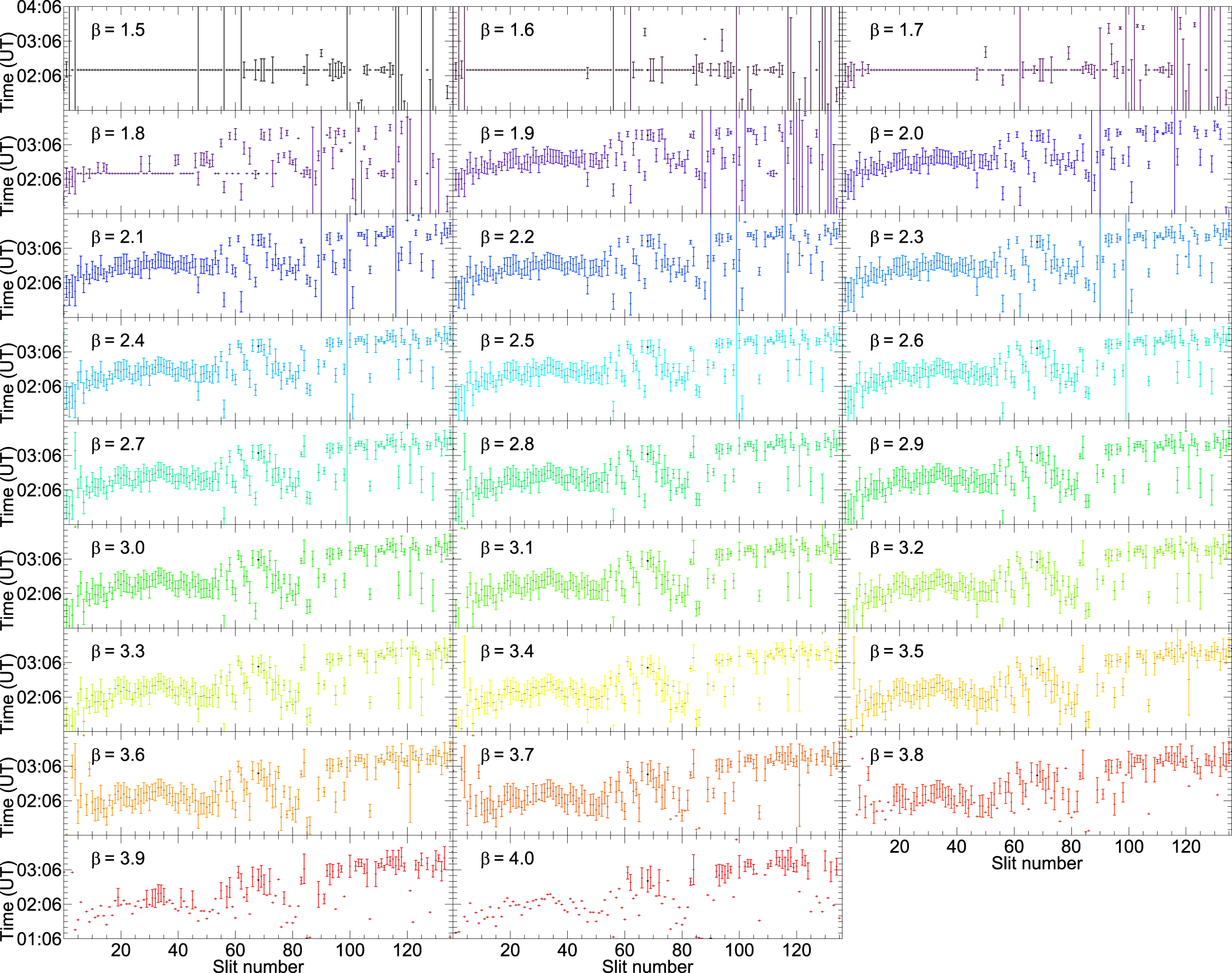
Figure B4. Acceleration multiplier, α.
Download figure:
Standard image High-resolution image
Footnotes
- 3
- 4
We also tested an exponential kinematic form by replacing the (t − tnl) polynomial with an equivalent (t − tnl) exponential. We omit the exponential functional fit analysis here because (a) we found that strict limits had to be placed on all of the free parameters, which is something that we want to avoid in this study, and (b) despite providing more appropriate convergence, the uncertainties returned for tnl are exceptionally large.
- 5