


Abstract
Particle-in-cell simulations show that numerous ion-scale magnetic islands can be formed in a turbulent magnetic reconnection region. These islands can confine and accelerate electrons to high energies effectively, causing the energetic electron energy flux to peak at the center of each island. ARTEMIS spacecraft observations of turbulent reconnection outflows in Earth's magnetotail reveal that peaks in the energetic electron energy flux are well correlated with bipolar signatures of reconnected magnetic field, which are indicative of ion-scale magnetic islands, providing observational evidence for this acceleration process.
Export citation and abstract BibTeX RIS
1. Introduction
How charged particles are accelerated to high energies in astrophysical systems has been a fundamental question for decades, and this question is particularly important for electrons because they can reach extremely high (relativistic) energies (Fermi 1949). Magnetic reconnection (Birn & Priest 2007; Yamada et al. 2010), a process of magnetic energy release and transfer to particles through topological changes in magnetic field lines, provides a good mechanism for particle acceleration. Reconnection is therefore widely believed to be responsible for energetic particle acceleration in various astrophysical plasma environments. For example, X-ray emissions in solar flares are thought to be caused by electrons accelerated to high energies (e.g., tens of keV) by magnetic reconnection (e.g., Lin & Hudson 1971, 1976; Masuda et al. 1994; Su et al. 2013). In Earth's magnetosphere, electrons with energies up to hundreds of keV have been directly detected at the reconnection region (Øieroset et al. 2002; Imada et al. 2007; Chen et al. 2008; Wang et al. 2010; Huang et al. 2012; Fu et al. 2013).
The classical understanding of electron acceleration by magnetic reconnection is based on a laminar reconnection scenario involving single X-line (or multiple separate X-lines). Electrons are accelerated by the reconnection electric field at the X-line(s) through a direct current acceleration process (e.g., Burkhart et al. 1990; Zelenyi et al. 1990; Øieroset et al. 2002; Fu et al. 2006; and references therein). In addition to the acceleration at the X-line(s), it has also been proposed that these electrons can be further accelerated in the reconnection exhaust region (Hoshino et al. 2001; Hoshino 2005; Pritchett 2006; Huang et al. 2010; Egedal. et al. 2012), which augments the acceleration efficiency of the laminar reconnection scenario.
Coherent structures, especially magnetic islands, produced by magnetic reconnection have also been found to play important roles in electron acceleration. Drake et al. (2006) proposed that contraction of magnetic islands can result in Fermi-type electron acceleration. Oka et al. (2010a) proposed that smaller islands with spatial scales on the order of ion kinetic scales can accelerate electrons via a surfing mechanism. These ion-scale islands are formed by secondary reconnection at the X-lines; therefore, they are referred to as secondary islands. Simulations also showed that coalescence of magnetic islands through an antireconnection process can also accelerate electrons (Pritchett 2008; Oka et al. 2010b; Tanaka et al. 2010, 2011). All of these magnetic islands with different spatial and temporal scales perturb sufficiently the ambient reconnection outflow region, leading to a new scenario—turbulent magnetic reconnection (e.g., Lazarian & Vishniac 1999; Daughton et al. 2011; Karimabadi et al. 2013; Fu et al. 2017; Cheng et al. 2018).
Using two-dimensional (2D) particle-in-cell (PIC) simulations, Lu et al. (2019b) examined electron acceleration in turbulent magnetic reconnection and found that ion-scale secondary magnetic islands have a high efficiency of electron acceleration. Therefore, electron acceleration in turbulent reconnection, which hosts many such islands, should be more efficient than electron acceleration in laminar reconnection. A systematic examination of this hypothesis using simulations and observations is needed. Here we present further evidence of this process in 2D PIC simulations, from a perspective of a direct comparison with observations (Section 2), and in situ observations from ARTEMIS confirming this hypothesis (Section 3). Sections 4 and 5 consist of a discussion and our conclusions.
2. PIC Simulations
In our 2D PIC simulation the electric and magnetic fields are defined on grids in the x–z plane and are updated by solving Maxwell's equations with a full explicit algorithm. The electrons and ions are treated as (macro)particles, with their motions governed by the equations of single particle motion. The initial magnetic field is B(z) = B0tanh(z/δ) ex, where B0 is the asymptotic magnetic field magnitude, δ is the current sheet half-width. The initial plasma consists of a Harris current sheet population and a background population, and the initial plasma density is  , where n0 is the peak density of the Harris current sheet, and nb is the background plasma density. Because an inhomogeneous temperature across the current sheet, with the background temperature Tb lower than the Harris current sheet temperature T0, has been shown to favor formation of secondary magnetic islands (Lu et al. 2019a, 2019b), we use
  . Specific parameters used are
  (di is the ion inertial length defined by n0),
  , the ion-to-electron mass ratio
  , and the speed of light
  (VA is the Alfvén speed evaluated using B0 and n0). The initial ion temperature is higher than the initial electron temperature by a factor of four, i.e.,
  , with
  and
and  for the Harris current sheet population. The initial background ion and electron temperatures are thus
  and
and  respectively. The grid size is
  , and the time step is
  , where
  is the unit ion gyrofrequency. The size of the simulation domain is
  and
and  . About
  particles are used in the simulation run. Periodic boundary conditions are used in the x direction; perfect conductor boundary conditions are used in the z direction.
Figure 1 shows the evolution of magnetic field lines and electron current density jey in the simulation. Magnetic reconnection with multiple X-lines emerges at about  and becomes better-developed at about
  . Magnetic islands, flanked by two X-lines, are also formed at the same time. We refer to these as primary islands and X-lines. Smaller magnetic islands are also formed at the primary X-lines through subsequent, secondary reconnection; we refer to these as secondary islands. Secondary islands differ from primary islands in three ways: (i) the spatial scale of secondary islands is smaller, on the order of several ion inertial lengths, compared to that of primary islands, which is on the order of several tens of ion inertial lengths. (In Earth's magnetotail, for example, these are ∼1000 km compared to about several Earth radii, respectively.) (ii) The lifetime of secondary islands is much shorter than that of primary islands, as secondary islands typically merge into primary islands. For example, the secondary island at about
  at
at  grows larger at Ωit = 70 and merges into the primary island on its right at
  . (iii) The out-of-plane electron current density jey is positive in secondary islands but negative in primary islands, as shown in Figures 1(c)–(e).
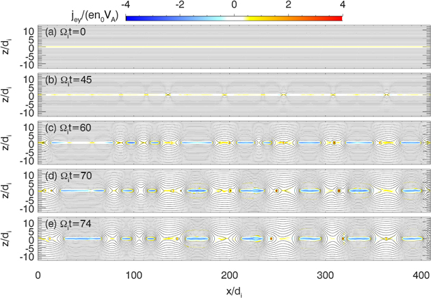
Figure 1. In-plane magnetic field lines and out-of-plane electron current density jey at representative moments,  , 45, 60, 70, and 74. The current density is in units of
  .
.
Download figure:
Standard image High-resolution imageAt Ωit = 70, there are seven secondary islands, which are characterized by bipolar Bz profiles at z = 0 (Figure 2, upper panels). The lower panels of Figure 2 show spatial profiles of integral high-energy electron energy flux "channels,"  , integrated above different energies,
  (different colors represent different channels). The highest channel,
  , corresponds to a Lorentz factor of
  . The high-energy electron energy flux peaks at or near the center of each secondary island, and the peak value is about one to two orders of magnitude higher than the ambient level. Therefore, such ion-scale secondary magnetic islands in turbulent reconnection can effectively confine and accelerate electrons to high or even relativistic energies.

Figure 2. Profiles of Bz (upper panels) and energetic electron energy flux (lower panels) along z = 0 for the seven secondary magnetic islands identified at Ωit = 70. The electron energy flux is defined as  (where
  is the electron kinetic energy), and it is integrated above 10 different energies,
  in 10 different high-energy ranges from
  to
to  , where
  is the initial current sheet temperature for electrons. The electron kinetic energy
  is in units of
  , and
, and  is the electron energy distribution, where
  . The electron density ne is in units of n0, so the energy flux is in units of
  .
.
Download figure:
Standard image High-resolution image3. ARTEMIS Observations
We seek confirmation of the above physical process using in situ observations of magnetic reconnection regions by the two ARTEMIS spacecraft (Angelopoulos 2011) in Earth's magnetotail. Orbiting the Moon, these spacecraft measure the plasma and magnetic field at a geocentric distance of about 60 Earth radii. Measurements at such large distances from the Earth allow us to probe the current sheet structure and reconnection outflows in a magnetic field configuration unperturbed by Earth's dipole. They provide an ideal data set for investigation of reconnection physics in a general current sheet. The ARTEMIS spacecraft detect reconnection regions embedded in both earthward and tailward plasma flows. The plasma flows are measured by the electrostatic analyzer (McFadden et al. 2008). The magnetic field is measured by the fluxgate magnetometer in Fast Survey mode of data capture with a time resolution of 0.25 s (Auster et al. 2008). Higher resolution magnetic field data (128 samples s−1) are available during Particle Burst mode, which can be used to resolve the fastest of events if the need arises, but have not been implemented on a statistical basis in this paper. To investigate high-energy electron energy fluxes, we use solid state telescope (SST) measurements (Angelopoulos 2008), which provide information about >30 keV electron energy fluxes. The typical electron temperature in the region under investigation is about several hundred eV (e.g., Wang et al. 2014; Artemyev et al. 2017b), and thus 30–70 keV electrons are high-energy electrons. The ion-scale islands have diameters of a few ion inertial lengths, about 1000–2000 km, and they move within the plasma flow at ∼200–400 km s−1. Therefore, these ion-scale islands move across the ARTEMIS spacecraft on a 3–10 s timescale. (Note that although there can be smaller scale islands, they cannot be resolved in Fast Survey, so they are not included in our data set.) This timescale is well-resolved in magnetic field data (0.25 s resolution) in our database, but not using the standard time resolution of SST data distribution functions (4 s, the spin period). Therefore, we utilize the 16 azimuthal angles of the SST instrument collected at equally spaced times during each spin, as separate measurements so that the SST time resolution is effectively increased to 1/4 s (see details of this method in Runov et al. 2011), which is similar to that from magnetic field data. This approach requires the assumption of electron gyrotropy, which is expected due to the electron gyroradius in a 3 nT field being comparable to an ion skin depth and the scale of the magnetic structures of the secondary plasmoid. This assumption has also been validated by examination of the electron velocity distributions obtained from PIC simulations (Lu et al. 2019b).
The reconnection outflows observed by ARTEMIS generally last for tens of minutes. Each such long-duration outflow consists of several bursts of flows with a duration of a few minutes. We selected 57 such bursts (see Table 1, each event in the table is one such burst) during which the plasma velocity magnitude exceeded 200 km s−1 at least once in the surrounding 10 minutes (the typical Alfvén speed in this region is 300–500 km s−1). Figure 3 shows one example of these events. Enhanced plasma flows are accompanied by magnetic field fluctuations. The typical reconnecting magnetic field (i.e., the field component normal to the reconnecting current sheet) is Bz in GSM coordinates. However, at such large distances from Earth the current sheet configuration is not well defined, and the standard GSM system does not necessarily coincide with the current sheet coordinate system. Therefore, we do not use magnetic field signatures to identify magnetic islands. Instead, we focus on observations of high-energy electron energy fluxes (Figure 3, lower panel). Although the spin resolution (4 s) measurements do not show any flux peaks, the subspin resolution (1/4 s) measurements exhibit many short peaks. To exclude the effects of transient fluctuations within only one of 16 azimuthal changes, we select only subintervals containing three-point peaks (peaks consist of at least three data points) of electron energy flux within 5 s or less. The main selection criteria of the subintervals are (1) three-point peak flux that is larger than the average value over three spin periods (12 s) around this peak; (2) three-point peak flux of 30–70 keV exceeds 10 cm−2 s−1 sr−1 (typical background flux amplitude); and (3) there is  , where
  is the Bz variation with respect to three-spin-period (12 s) average. We additionally examine all the selected subintervals and exclude the subintervals containing random single-point peaks of electron fluxes (see the number of subintervals for each outflow event in Table 1).

Figure 3. One sample event from our data set. (a) Magnetic field components Bx (black), By (red), and Bz (blue). Generally, Bx and By are reconnecting magnetic field components, and Bz is a reconnected magnetic field component. (b) Plasma flow velocity Vx (<−200 km s−1) in the reconnection outflow region. (c) SST electron energy fluxes for spin (4 s) resolution (in black) and subspin 4/16 = 1/4 s resolution (shown by yellow circles).
Download figure:
Standard image High-resolution imageTable 1. List of Turbulent Reconnection Outflow Events in which ARTEMIS P1 or P2 Observed Ion-scale Magnetic Islands (the Number of such Islands N in Each Event is Shown in the Last Column).
| Date and Time Interval | sc | N |
|---|---|---|
| 2014 Jan 15 02:00–03:00 | P1 | 1 |
| 2014 Jan 16 06:00–07:00 | P1 | 2 |
| 2014 Feb 14 20:00–21:00 | P1 | 1 |
| 2014 Feb 15 01:00–02:00 | P1 | 1 |
| 2014 Mar 15 05:00–07:00 | P1 | 3 |
| 2014 Mar 16 04:00–06:00 | P1 | 3 |
| 2014 Apr 14 02:00–03:00 | P2 | 3 |
| 2014 Apr 14 06:00–07:00 | P1 | 1 |
| 2014 Apr 14 22:00–23:50 | P1 | 3 |
| 2014 May 13 20:00–21:00 | P1 | 1 |
| 2014 Jun 11 15:00–17:00 | P1 | 4 |
| 2014 Jun 12 05:00–06:00 | P1 | 2 |
| 2014 Jun 13 09:00–10:00 | P2 | 1 |
| 2014 Oct 7 04:00–05:00 | P1 | 3 |
| 2014 Nov 5 16:00–17:00 | P1 | 2 |
| 2014 Nov 6 21:00–22:00 | P1 | 2 |
| 2015 Jan 5 01:00–02:00 | P2 | 1 |
| 2015 Feb 3 10:00–11:00 | P2 | 3 |
| 2015 Mar 4 12:00–13:00 | P1 | 2 |
| 2015 May 3 16:00–17:00 | P2 | 3 |
| 2015 Jul 1 01:00–02:00 | P2 | 4 |
| 2015 Jul 31 14:00–15:00 | P1 | 4 |
| 2015 Sep 26 23:00–23:50 | P1 | 1 |
| 2015 Dec 24 12:00–13:00 | P2 | 1 |
| 2016 Feb 23 00:00–01:00 | P2 | 1 |
| 2016 Mar 23 08:00–09:00 | P2 | 3 |
| 2016 Apr 21 20:00–22:00 | P2 | 3 |
| 2016 May 21 15:00–16:00 | P2 | 3 |
| 2016 Jun 19 06:00–08:00 | P1 | 1 |
| 2016 Jul 19 02:00–03:00 | P1 | 1 |
| 2016 Sep 16 17:00–18:00 | P2 | 1 |
| 2016 Nov 13 00:00–01:00 | P2 | 1 |
| 2016 Nov 14 09:00–10:00 | P2 | 1 |
| 2016 Dec 13 03:00–04:00 | P1 | 2 |
| 2017 Feb 11 01:00–02:00 | P2 | 4 |
| 2017 Mar 11 22:00–23:50 | P2 | 5 |
| 2017 Mar 12 00:00–01:00 | P2 | 3 |
| 2017 Apr 10 01:00–02:00 | P2 | 1 |
| 2017 Apr 10 15:00–16:00 | P1 | 6 |
| 2017 Apr 11 09:00–10:00 | P1 | 3 |
| 2017 Jul 7 16:00–18:00 | P1 | 5 |
| 2017 Aug 7 08:00–09:00 | P2 | 1 |
| 2017 Nov 3 09:00–11:00 | P2 | 5 |
| 2017 Dec 2 15:00–16:00 | P1 | 1 |
| 2017 Dec 3 22:00–23:00 | P1 | 2 |
| 2018 Mar 2 08:00–09:00 | P2 | 2 |
| 2018 May 29 04:00–05:00 | P2 | 5 |
| 2018 Jul 27 06:00–07:00 | P2 | 2 |
| 2018 Aug 25 14:00–15:00 | P1 | 3 |
| 2018 Aug 26 15:00–16:00 | P2 | 3 |
| 2018 Sep 24 10:00–11:00 | P2 | 1 |
| 2018 Sep 25 11:00–13:00 | P2 | 2 |
| 2018 Nov 22 08:00–09:00 | P2 | 2 |
| 2018 Nov 23 10:00–11:00 | P1 | 1 |
| 2018 Dec 21 08:00–10:00 | P1 | 2 |
| 2018 Dec 22 11:00–12:00 | P2 | 1 |
| 2018 Dec 22 16:00–17:00 | P1 | 2 |
Download table as: ASCIITypeset image
For all these intervals we transform the time to a space coordinate, x, using the measured plasma velocity, and normalize this coordinate in the ion inertial length, di, evaluated using the average ion density. In this method, x is always in the direction of island propagation (regardless of whether that is tailward or earthward). Next, we examine δBz for the intervals with electron energy flux peaks. Figure 4 shows four examples of δBz fluctuations and electron energy fluxes. An interesting feature is that each electron energy flux peak almost always coincides with a bipolar fluctuation of δBz. Such correlations indicate that the observed electron energy flux peaks could be attributed to magnetic structures such as magnetic islands or X-lines. Upon closer inspection, for the majority of such fluctuations,  at
at  and
and  at
at  . This δBz profile (similar to those in simulations as seen in Figure 2, upper panels) is consistent with a tailward-moving magnetic island configuration; tailward-moving secondary islands appear to dominate our observational database.

Figure 4. Four examples of electron energy flux peaks observed in the reconnection outflow. For each event we show detrended magnetic field configuration and electron energy flux for two energy ranges (both spin and subspin resolutions are shown). Time is transferred to the space coordinate (normalized to the ion inertial length) using plasma flow speed.
Download figure:
Standard image High-resolution imageAlthough electron energy flux peaks can be observed in both the 30–70 keV and the 70–100 keV range in some intervals (see Figure 4), the 70–100 keV electron energy fluxes are usually weak and their variations are not as clear as those of 30–70 keV fluxes. Therefore, we focus on 30–70 keV flux peaks and collect them into an epoch analysis (the total number of intervals with such peaks is 131). For each interval we determine a typical timescale T (during which electron energy flux j varies from  to jmax and then back to
  , where jmax is the three-point peak value of electron energy flux) and typical spatial scale
  . Figures 5(a) and (b) show the superposed epoch analysis of the normalized electron energy flux and δBz. The 30–70 keV electron energy flux peaks are clearly seen to be statistically associated with bipolar Bz variations, which are indicative of magnetic islands. As evident from Figure 5(c), the electron energy flux peaks and the δBz have a spatial scale of
  (where the ion inertial length, di, is evaluated using the averaged ion density), confirming that the magnetic islands are indeed ion-scale secondary islands. Consistent with the predominance of positive-then-negative profiles in δBz (bespeaking of predominantly tailward-moving secondary islands), Figure 5(e) shows that most of our events are embedded within tailward flows (Vx < 0). Considering that the probabilities of observing tailward and earthward flows by ARTEMIS are approximately equal in this region (see Kiehas et al. 2018), we conclude that the observed asymmetry is not an orbital or observational bias in the original database. Such asymmetry is likely because that magnetic reconnection on the earthward side of ARTEMIS (resulting in tailward flows) is more powerful than on the tailward side of ARTEMIS possibly due to the larger Alfvén velocity and higher reconnection rate closer to Earth (Artemyev et al. 2017a).
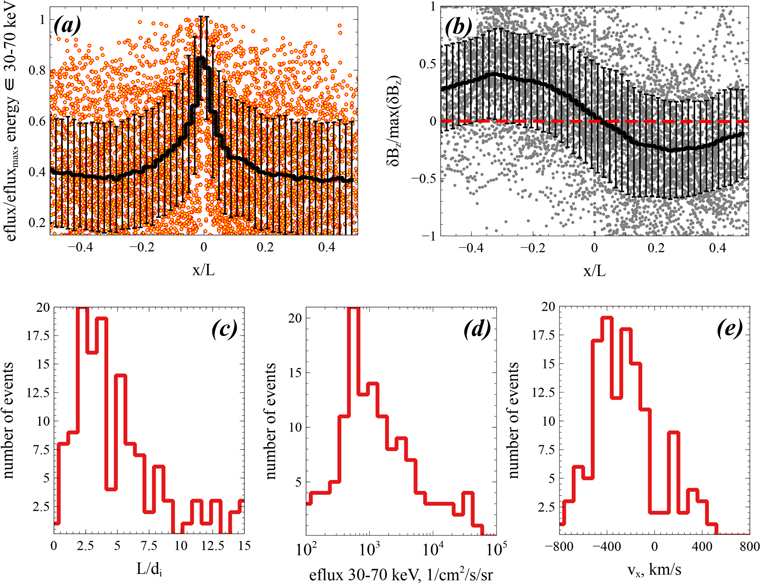
Figure 5. Superposed epoch analysis and event distributions for short electron energy flux peak events. (a), (b) Averaged profiles of normalized electron energy fluxes and magnetic field fluctuations. (c), (d), and (e) Distributions of spatial scales of magnetic field fluctuations, peak values of electron energy flux, and plasma velocity, respectively.
Download figure:
Standard image High-resolution imageThe electrons accelerated within these ion-scale magnetic islands can form electron beams and temperature anisotropies, which are unstable to wave growth (e.g., Gary 2005). Therefore, observations of electron-driven waves at these islands serve as an additional indicator of electron acceleration to unstable velocity distributions. Figure 6 shows electric field spectra averaged over all the observed islands in our database. The electric field power was normalized to the background level (prior to each event). Averaging was performed over different distances from the island center (ahead of, during, and past the central region). There is a clear peak around ∼4–7 kHz (the electron plasma frequency in the region of ARTEMIS observations is about 5 kHz). The wave power intensity in this frequency range decays with the distance from the island center. Electrostatic wave emissions around the electron plasma frequency can be caused by the accelerated electrons, which further supports our hypothesis of electron acceleration within the ion-scale secondary islands.
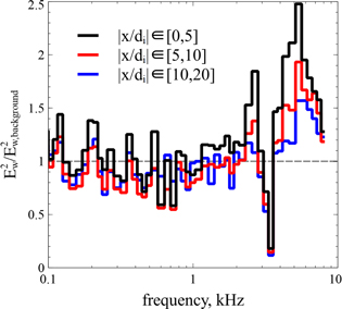
Figure 6. Electric field wave spectrum (see details of wave measurements and data processing in Bonnell et al. 2008; Cully et al. 2008) normalized to the background level for three ranges of the distances around the peak of high-energy electron energy fluxes.
Download figure:
Standard image High-resolution image4. Discussion
Our PIC simulations and ARTEMIS observations both show energetic electrons accelerated by ion-scale magnetic islands, the energetic electrons detected by ARTEMIS, however, extend to higher energies (several hundred times the thermal energy) than in the PIC simulations (several tens of the thermal energy). One reason for this quantitative difference could be that the simulations have a limited number of particles (macroparticles) and is unable to properly reveal the acceleration of the few very high-energy electrons (the phase space density is exponentially smaller at the highest energies). As shown in Figure 2, at  , the peak number flux for
  is about
  , corresponding to about 12 particles in the simulation. For higher energies, such as a hundred times the thermal energy, the number flux falls dramatically so that the number of particles is much less than 12, which is not statistically significant. Another possible reason could be that our simulations do not fully reproduce the energetic particle acceleration efficiency, which is discussed as follows.
- 1.Energetic electrons can be accelerated in single ion-scale secondary islands through the island surfing mechanism (Oka et al. 2010a). These single secondary islands can merge and form new islands (Wang et al. 2016), during which the electrons can be further accelerated through Fermi acceleration (Drake et al. 2013; Dahlin et al. 2014; Zank et al. 2014; Li et al. 2017; le Roux et al. 2018). However, in our PIC simulations, the merger between secondary islands does not show; therefore, the electron acceleration efficiency may be underestimated because of the absence of the Fermi acceleration resulting from island merger.
- 2.Magnetotail reconnection is mostly antiparallel because the out-of-plane guide field therein is usually weak (e.g., Petrukovich 2011; Rong et al. 2011); therefore, our PIC simulations are based on the antiparallel reconnection scenario with zero guide field. However, in the magnetotail and other astrophysical environments, strong guide fields may exist, in the presence of which, the electron acceleration mechanism in ion-scale secondary islands changes—no longer through island surfing acceleration (Oka et al. 2010a) but through parallel electric acceleration (Wang et al. 2017) and/or adiabatic betatron and Fermi acceleration (Zhong et al. 2020). This change of electron acceleration mechanisms can also lead to the change of acceleration efficiency.
- 3.In our 2D simulations, which assume infinite length and uniformity in the y direction, the lifetime of the secondary islands in the 2D turbulent reconnection is
 . Therefore, in the lifetime of a secondary island, an energetic electron accelerated to by this island can move in the y direction. If the y-extent of the secondary islands is much less than 100di, it is plausible that our 2D simulations overestimate the electron acceleration efficiency in the secondary islands. However, in the realistic 3D turbulent reconnection, which hosts numerous magnetic islands with finite y-extent, the electrons are no longer confined to single island but, rather, wander across multiple islands, which favors stochastic acceleration or second-order Fermi acceleration (e.g., Zank et al. 2014; le Roux et al. 2018; Zhao et al. 2018, 2019). This different electron trajectories result in different acceleration efficiencies between 2D and 3D, and the PIC simulations by Dahlin et al. (2015) do show that the electron acceleration efficiency is higher in 3D.


Finally, our simulations use periodic boundary conditions in the x direction. Previous simulations have shown that the use of open boundary conditions in the x direction favors the formation of secondary islands (e.g., Daughton et al. 2006; Klimas et al. 2008), therefore, one would expect even more secondary islands, and more energetic electrons accelerated within them, if open boundary conditions are used.
5. Conclusions
We have shown through PIC simulations that numerous ion-scale secondary magnetic islands formed in the vicinity of a magnetic reconnection region can accelerate energetic electrons effectively. The ARTEMIS spacecraft, in Earth's magnetotail at lunar distance, observed ion-scale peaks of high-energy electron energy fluxes (energies a factor of ∼100 higher than the electron temperature) in turbulent reconnection outflows. These electron energy flux peaks have a spatial scale of several ion inertial lengths and correlate with bipolar (±) variations of the magnetic field normal to the current sheet, Bz, which is indicative of ion-scale magnetic islands. These observations support our hypothesis from simulations that ion-scale magnetic islands significantly accelerate energetic electrons in turbulent reconnection.
This work was supported by NASA contract NAS5-02099 and NASA grants NNX17AI46G and 80NSSC18K1122. We would like to thank the following people specifically C. W. Carlson and J. P. McFadden for the use of ESA data, D. E. Larson and R. P. Lin for the use of SST data, and K. H. Glassmeier, U. Auster, and W. Baumjohann for the use of FGM data provided under the lead of the Technical University of Braunschweig and with financial support through the German Ministry for Economy and Technology and the German Aerospace Center (DLR) under contract 50 OC 0302. We thank J. Hohl for her assistance in preparation and editing of this paper. The THEMIS data were downloaded from http://themis.ssl.berkeley.edu/. The computer resources were provided by the NASA High-End Computing (HEC) Program through the NASA Advanced Supercomputing (NAS) Division at Ames Research Center.