


Abstract
We analyze archival Chandra X-ray Observatory observations of Jupiter to search for emission from the Galilean moons. X-ray emission has previously been reported from Io and Europa using a subset of these data. We confirm this detection, and marginally detect X-ray emission from both Ganymede and Callisto as well. The X-ray spectrum of Europa is strongly peaked around the neutral oxygen fluorescence line (525 eV), while Io's has peaks at both oxygen and sulfur (2308 eV) plus a broad continuum between 350 and 5000 eV. Ganymede's spectrum is similar to Io's, but without the sulfur peak. A few events, mostly clustered around the oxygen line, are detected from Callisto. Using measurements by the Galileo mission of the specific intensity of ambient protons and electrons, we model the X-ray spectra and flux of the moons from two processes: particle-induced X-ray emission (PIXE) from the impact of energetic protons and X-ray emission from electron bremsstrahlung. With uncertainties of a factor of a few, the electron bremsstrahlung and PIXE models overestimate the X-ray flux from Europa, preventing us from making a definitive statement about the origin of the X-ray emission. The PIXE model of Io predicts emission lines at O and S similar to those observed, but underestimates their flux by nearly two orders of magnitude. Based on this discrepancy in the PIXE flux, combined with the detected broadband continuum in the spectrum, we conclude that the X-ray emission from Io is due to electron bremsstrahlung. Likewise, because of Ganymede's broad continuum, we tentatively conclude that its X-ray emission is also due to electron bremsstrahlung. Callisto is too faint in the X-rays to draw any conclusion. Obtaining in situ X-ray observations of the moons would provide a direct measurement of their elemental composition.
Export citation and abstract BibTeX RIS
1. Introduction
A variety of endogenic and exogenic processes shape the surfaces of the Galilean moons. Their surfaces are continually exchanging material with their atmospheres and hence with the Jovian magnetosphere. Surface material can enter the atmosphere via sublimation (or even evaporation) or sputtering. From there, it can escape the moon into the neutral clouds or the Io plasma torus, or it can recondense elsewhere on the surface. The trailing sides of both Io and Europa are bombarded with ions from the Io plasma torus, while the leading sides of the moons, due to the orbital motion, will receive impacts from a disproportionate quantity of cometary micrometeoroids, ejecta from other Jovian moons, and material from beyond the Jovian system. The surfaces also exchange material with the interior. Micrometeoroid gardening can bury the surface and expose a fresh surface. Spectacular volcanic eruptions on Io eject large quantities of solid, liquid, and gaseous material into the atmosphere; from there, it can escape the moon or fall down to coat the surface. Tectonic activity on both Io and Europa can also bring material to the surface. Plumes of water have been putatively observed erupting from the surface of Europa (Roth et al. 2014; Sparks et al. 2017). This provides another possible mechanism for the briny water from the subsurface ocean to reach the surface, providing an opportunity for the composition of its salts and other components to be examined. Thus, knowledge of the surface composition of the Galilean moons provides information not only about the surface itself, but also about the interior of the moon, its atmosphere, and its extended environment.
The surface of Io is constantly changing because of the moon's active volcanism, the large temperature variations due to its orbital motion around Jupiter, and the continuous bombardment from charged particles in the Jovian magnetosphere. A compilation of near-UV to near-IR reflectance measurements of the surface of Io demonstrate the presence of SO2, various allotropes of S, H2O, H2S, Cl2SO2, as well as a variety of other sulfates and salts (Spencer et al. 2004). One of the complications with interpreting the reflectance spectrum of Io is that this spectrum can be easily modified by small amounts of elements (Kargel et al. 1999). A thin layer of SO2 may cover much of Io as a frost (Howell et al. 1984). Models of the formation of Io suggest the presence of silicates, but the observational evidence of such material in the surface is ambiguous at best. In particular, it has been argued, based on Galileo SSI imaging, that there are Mg-rich silicates present in the surface of Io (McEwen et al. 1998). Direct measurements of elements such as Na, Mg, and K in the surface of Io could have important implications for modeling the formation of this moon and the evolution of its crust, mantle, and core.
The Galileo Near-Infrared Mapping Spectrometer (NIMS) provided a wealth of information about the surface composition of Europa using reflected sunlight and thermal radiation to collect spectra arising from molecular vibrational transitions of both solid and gaseous species (Carlson et al. 1996). The paucity of craters indicate that the surface of Europa is geologically young (40–90 Myr), so it is continually being eroded and resurfaced. Europa has two distinct hemispheres. The leading side has a bright surface of predominantly water ice with very low hydrate concentration (Carlson et al. 2009), whereas the trailing side has a reddish-brown surface. Micrometeoric deposition would occur mainly on the leading white side. Distortions of the water spectrum from the trailing red hemisphere indicate that most of the water present is in the form of hydrates (Carlson et al. 2009). The hydrates have a bullseye distribution on the red, trailing side (Dalton 2007), with a maximum concentration of around 80% or 90%. This concentration is nine times that of free water, according to Carlson et al. (2005). Carlson et al. (2009) were able to replicate a NIMS spectrum with, for example, a linear combination of cryogenic reflectance spectra using 62% sulfuric acid hydrate, 14% hexahydrite, 11% bloedite, and 12% mirabilite with no free water. Other combinations of hydrates provided comparable results. Observed portions of the white, leading hemisphere show a hydrate concentration of around one ninth that of free water. More recently, Brown & Hand (2013), using adaptive optics and the OSIRIS integral field spectrograph at the W. M. Keck Observatory, found a signature of MgSO4 on the trailing side of Europa and concluded that it was a radiation product of MgCl2. They therefore predicted the presence of sodium and potassium chlorides. Experiments by Hand & Carlson (2015) found that exposing sodium chloride to conditions like those at Europa's surface yields a yellow-brown color similar to the non-ice material observed on Europa. The presence of significant amounts of chlorine on the surface of Europa is supported by Ligier et al. (2016), who used near-infrared spectra from an integrated field unit spectrometer on ESO's Very Large Telescope at the La Silla Paranal Observatory and found their best fits for combinations of water, sulfuric acid hydrate, and Mg-bearing chlorinated salts (chloride, chlorate, and perchlorate). Infrared reflectance and thermal spectroscopy probe the chemical bonds of the surface but are not as sensitive to the elemental composition.
The near-UV to near-IR spectroscopic measurements provide a wealth of information about the broad classes of chemical compounds present in the surfaces of Io and Europa, but many key questions remain. What is the precise state of the silicates? What is the reddish-brown material on the surface of Europa? Are the non-water components of Europa's surface dominated by compounds of sulfur or of chlorine? Are there any trace elements present? If so, how are they distributed, and what does this tell us about the interaction of the surface with the Jovian magnetosphere, the atmosphere, and in Europa's case, the subsurface ocean?
In the presence of ionizing radiation, sensitive X-ray spectroscopic measurements would, in principle, provide detailed stoichiometry and directly measure the abundance of trace elements. Such measurements are commonplace on airless rocky bodies, such as the Moon and Mercury, where characteristic X-ray lines are generated by absorption of solar coronal X-rays. The Galilean moons are too far from the Sun for this to be an efficient mechanism for the generation of X-rays. Fortunately, the Galilean moons reside inside one of the best nonthermal particle accelerators in the solar system: the Jovian magnetosphere. Energetic electrons and protons in the magnetosphere strike the surface of the moons and generate characteristic X-rays. An X-ray fluorescence spectrum would be able to unambiguously distinguish between the two above models for the composition of Europa, in addition to identifying other elements present in trace amounts undetectable through near-IR spectroscopy.
In this paper, we reanalyze archival Chandra X-ray Observatory observations of the Galilean moons and confirm the detections of X-ray emission from both Io and Europa reported by Elsner et al. (2002). We also find X-ray emission from Ganymede and possibly Callisto. We then model the interaction of the energetic electron and proton populations with the surfaces of these moons to compare with the observed spectra and fluxes. We use the thick-target bremsstrahlung model to predict the X-ray emission from the electron precipitation (Pella et al. 1985) and particle-induced X-ray emission (PIXE) to model the X-ray emission produced by the proton precipitation (Maxwell et al. 1989, 1995), making simplifying assumptions about the geometry. We find that the X-ray emission from Io is described well by the electron bremsstrahlung model, and that PIXE is not an important process for the generation of X-rays there. The emission from Europa is overpredicted by a factor of a few by both the PIXE and the electron bremsstrahlung models, and we cannot make a definitive statement. Due to the presence of an X-ray continuum, we argue that, like Io's X-ray emission, the emission from Ganymede is better described by the electron bremsstrahlung model. Too few X-ray photons have been observed from Callisto to distinguish between the models. We discuss the implications of our results. The quality of the data in the present study is too limited to allow for detailed measurements of elemental abundances. However, a dedicated instrument would achieve a count rate around seven orders of magnitude larger than in the existing Chandra data.
This paper is organized as follows. In Section 2, we discuss the Chandra data and our analysis technique. We describe our modeling of the X-ray emission using PIXE and thick-target bremsstrahlung in Section 3. A detailed comparison of the data with our models is presented in Section 4. Section 5 gives a brief summary and discusses the implications of these results.
2. Data Analysis
Chandra has observed Jupiter 14 times with the ACIS instrument since the beginning of the mission, and 15 times with the HRC by the time of our analysis. Elsner et al. (2002) reported the detection of X-ray emission from Io and Europa based on early observations of the Jovian system with the Chandra X-ray Observatory using both the ACIS and HRC instruments. See Elsner et al. (2002) for X-ray images of Io and Europa. Early in the mission, the ACIS instrument was preferred because of its significantly lower internal background and moderate energy resolution. All of the observations of Jupiter since 2011, however, have been made with the HRC, as contamination building up on the ACIS instrument has slowly decreased the low energy (<1 keV) sensitivity (Plucinsky et al. 2018). In this work, we reanalyzed all of the archival ACIS observations of the Galilean moons to confirm the results of Elsner et al. (2002) and to extract the X-ray spectra and fluxes to compare with our model predictions. Table 1 shows a summary of all the ACIS X-ray observations used in this work.
Table 1. Summary of ACIS Observations of the Galilean Moons
| ObsID | Date | teff (s) | |||
|---|---|---|---|---|---|
| Io | Europa | Ganymede | Callisto | ||
| 1 | 99 Nov 25 | 12660 | 21180 | 21180 | 21180 |
| 960 | 99 Nov 25 | 23520 | 23520 | 23520 | 23520 |
| 1463 | 99 Nov 26 | 16080 | 24600 | 24600 | 24600 |
| 1482 | 99 Nov 25 | 20040 | 20040 | 20040 | 20040 |
| 3726 | 03 Feb 24 | 27120 | 31500 | 26280 | 31500 |
| 4418 | 03 Feb 25 | 34320 | 32040 | 43200 | 43200 |
| 7405 | 07 Feb 8 | 18960 | 18960 | 18960 | 18900 |
| 8216 | 07 Feb 10 | 10980 | 19620 | 19620 | 19620 |
| 8217 | 07 Feb 24 | 10920 | 17580 | 17580 | 17580 |
| 8218 | 07 Mar 8 | 20520 | 20520 | 20520 | 20520 |
| 8219 | 07 Mar 3 | 19200 | 19200 | 19200 | 19200 |
| 8220 | 07 Mar 7 | 8700 | 17340 | 17340 | 17340 |
| 12315 | 11 Oct 2 | 40620 | 41640 | 32880 | 41640 |
| 12316 | 11 Oct 4 | 42300 | 42300 | 42300 | 42300 |
| Total ACIS times | 305940 | 350040 | 347220 | 361140 | |
Note. The effective observation times, teff, are in seconds after removing transits of the Jovian disk.
Download table as: ASCIITypeset image
The X-ray emission from each of the Galilean moons was extracted from a circle with a radius of three times its projected angular radius. Instrumental background was determined in an annular region extending to twice this distance. Scaling by area, one-third of the number of counts detected in this annulus were used to estimate the background for the area in which counts from the moon were measured. The coordinates of the moon from the viewing position of Chandra during each observation were determined using the JPL Horizons web interface (https://ssd.jpl.nasa.gov/horizons.cgi). The position data were binned on intervals of 100 s and the position interpolated to the 3.2 s ACIS frame time. The motion of Chandra is sufficiently small in this interval that the apparent motion of the moon is significantly less than the angular resolution of the telescope. We also exclude times when the apparent position of the moon is within 1.1 RJ of the center of Jupiter. The disk of Jupiter is a bright source of scattered solar X-rays, and the bias frames of several of the early ACIS observations are compromised due to an optical light leak that was not correctly accounted for, falsely generating a large number of low-energy events at the limb of the planet. This correction is generally small for Europa, but is larger than 50% for several of the Io observations. For Io, 69% of the time the face viewed was predominantly the leading hemisphere. For Europa, Ganymede, and Callisto, this proportion was 28%, 37%, and 60%, respectively. However, due to the small numbers of counts, no attempt was made to determine which faces of the moons were observed. The effective observation times excluding Jovian transits are summarized in Table 1.
Totals of 24 and 15 counts in the 0.5–5.0 keV band were detected from Io and Europa, respectively, in the 14 observations over a total of ∼360 ks of observing time. Subtracting the estimated background counts gives 21 ± 5 and 13 ± 4 counts, respectively, from Io and Europa. We therefore confirm at >99% confidence the detection of these Galilean moons as X-ray sources as first reported by Elsner et al. (2002). The extracted energy spectra, from 0.35 to 5.0 keV, of the two moons are shown in the upper two panels of Figure 1. The observed X-ray spectrum of Europa is strongly concentrated around 0.5 keV, indicative of emission from neutral O. The spectrum of Io is more broadly distributed across the band with peaks at O (0.525 keV) and S (2.308 keV). To show the locations of these emission lines, Figure 1 contains Gaussian lines with the instrumental resolution overplotted on the data at the Kα energies of O (0.525 keV), Na (1.041 keV), and S (2.308 keV). The Gaussian heights roughly follow peaks in the counts.

Figure 1. X-ray spectra of each of the Galilean moons, using 50 eV energy bins, overlaid with Gaussians at the positions of the O Kα (0.525 keV), Na Kα (1.041 keV), and S Kα (2.308 keV) lines.
Download figure:
Standard image High-resolution imageFinally, we repeated this analysis for both Ganymede and Callisto. A marginal detection was reported for Ganymede by Elsner et al. (2002). Using our much larger data set, we are able to detect X-ray emission from Ganymede with 11 ± 4 counts, after removing the background, in ∼350 ks, giving a detection at >99% confidence. The spectrum of Ganymede was similar to Io's except for the absence of a clear sulfur peak. It had a continuum at energies that could not be ascribed to elemental characteristic lines; see the bottom left panel of Figure 1. Over a time of 361.2 ks, three counts were seen from Callisto in the 0.5–5 keV band (four in the 0.35–5 keV band), leaving only 2 ± 2 counts after subtracting the background. However, there is a peak around the energy of the O line, indicating that this is most likely a detection of oxygen X-rays. See the bottom right panel of Figure 1.
2.1. Spectral Analysis
To make a more quantitative description of the X-ray spectra from Io and Europa, we attempted to fit simple models to each. We acknowledge that, given the low numbers of counts and the distribution of the detected events over several observing cycles, our results should be regarded as suggestive at best. Virtually all of the photons were detected prior to AO5 before the contamination became a serious issue for ACIS. We therefore created spectra using our event list and generated RMF and ARF files relevant to an AO3 ACIS-S observation. We created our spectra in PI space, making them uniform in gain across the observations, but there may well be subtleties in the redistribution that we do not account for. Given the small number of counts in both spectra and the potential systematics of this procedure, our ability to draw strong conclusions is limited.
We fitted two models to the spectra of Io. In the first model, we included only emission lines from O and S (i.e., a PIXE model spectrum). This model can be rejected immediately, as it does not account for the broad emission between these two strong emission lines. We fitted a second model including O Kα (525 eV) and S Kα (2308 eV) emission lines and a power-law continuum (i.e., an electron bremsstrahlung model spectrum). The power-law index of the continuum model is fixed at the value determined from our bremsstrahlung model (see below), but our results are insensitive to this restriction. The data and model fit for this spectrum are shown in Figure 2. Note that, in a formal statistical sense, the fit is still poor ( ), but clearly the data require a model with both the emission lines and the continuum. The observed width of the lines is not well-captured in our model, and almost certainly reflects systematics due to our ad hoc response matrix.
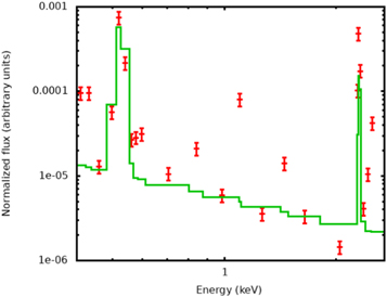
Figure 2. Data and best-fit model (emission lines at O Kα (0.525 keV) and S Kα (2.308 keV) plus power-law continuum) for Io X-ray spectrum.
Download figure:
Standard image High-resolution imageLikewise, we fitted two models to the X-ray spectrum of Europa, the first of two emission lines at O Kα (525 eV) and Na Kα (1041 eV), and a second model consisting of these two emission lines plus a power law to model the bremsstrahlung continuum. Both models are equally poor descriptions of the data ( ). The data and second model (two Gaussian lines plus power-law continuum) are shown in Figure 3. There are simply too few counts and the spectral quality is too low for us to definitively distinguish between these models based on X-ray spectrum.

Figure 3. Data and best-fit model (emission lines at O Kα (0.525 keV) and Na Kα (1.041 keV) plus power-law continuum) for Europa X-ray spectrum.
Download figure:
Standard image High-resolution image3. Modeling
We confirm the results of Elsner et al. (2002) and detect X-ray emission from both Io and Europa. We now consider two models for the X-ray emission: PIXE and thick target electron bremsstrahlung. The Jovian magnetosphere is an efficient nonthermal particle accelerator, and we assume that the thin exospheres of these two moons offer no impediment to energetic particles striking their surfaces and generating X-rays. In this work, we use the proton (for PIXE) and electron (for bremsstrahlung) intensities measured by Galileo to estimate the X-ray fluxes. Given the limited quality of the X-ray data (a few tens of counts total), several important simplifications are made to facilitate comparison of the data with the models. First, we assume that the moons are spherical and embedded in an azimuthally symmetric particle distribution. Second, we assume simplified elemental surface compositions of the two moons. Third, we ignore any effects of the moons' orbits around Jupiter. We make no attempt to distinguish leading and trailing emission in either the modeling or data analysis. Europa in particular is known to have significant compositional differences in the leading and trailing sides. These differences could be the focus of a future investigation. Fourth, we ignore the complexities of limb brightening or limb darkening, and assume that the average X-ray intensity is well-modeled by using the case of a 45° incident angle and an identical takeoff angle. We note that, while other emission mechanisms such as charge-exchange are not formally excluded by the data, they seem highly implausible. The Galilean moons are almost always within the Jovian magnetosphere, and thus are rarely exposed to the highly ionized solar wind. Additionally, simple scalings based on size and atmospheric density with the X-ray emission detected from Mars (Dennerl 2002) make this scenario implausible.
3.1. Particle-induced X-Ray Emission (PIXE)
One possible source of these X-rays is PIXE (Johansson et al. 1995). When energetic protons in the 0.1–10 MeV range strike the surface of the moons they will produce inner (K and L) shell ionizations and generate characteristic X-rays. An X-ray spectrometer with moderate spectral resolution can be used to determine the elemental composition of a sample bombarded by these energetic ions. PIXE is commonly used in a wide range of terrestrial applications for nondestructive determination of the elemental composition of works of art and in industrial settings. The models and underlying physical assumptions are well-understood and well-tested. The Galilean moons provide a natural laboratory for application of this technique. The high-energy protons and ions of helium, sulfur, and oxygen present in the Jovian magnetosphere provide the radiation source that excites atoms on the surface of the moon.
The X-ray flux, FL, of a characteristic emission line L with energy EL due to PIXE from one of the moons, in units of  , is given by
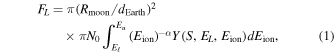
where  and
and  are the radius of the moon and distance between the moon and Earth, respectively, Eion is the proton energy in keV, N0 and α are the normalization and spectral energy index of the proton spectrum (assumed to be a power law with N0 in units of
  ),
),  and Eu are the lower and upper proton energies (assumed to be 0.1 and 10 MeV in our analysis), EL is the characteristic line energy of the relevant element, S is the surface composition with the fraction of each element in the surface material given in units of parts per thousand (ppt) by mass, and Y is the PIXE yield in units of
  . Throughout this paper, compositions are expressed in terms of parts per thousand (ppt) by mass.
We employed the GUPIX (Guelph University PIXe) software package to compute the PIXE yields from the Galilean moons. GUPIX is a widely used software package (http://pixe.physics.uoguelph.ca/gupix/main/) produced by the PIXE group at the University of Guelph to model the PIXE emission from targets of any material impacted by energetic protons at arbitrary impact and takeoff angles. The GUPIX code uses nonlinear least-squares fitting of Si-resolution X-ray spectra to derive element concentrations from the areas of X-ray peaks in the spectrum. It has been well-tested both with laboratory measurements and via comparisons with other PIXE codes (Blaauw et al. 2002). Our scenario is the inverse problem, in that we have an assumed particle distribution and surface material and want to compute the X-ray yields. The GUYLS program from the GUPIX package makes this calculation incorporating all the relevant atomic physics (Johansson et al. 1995), and was kindly supplied by Dr. John (Iain) L. Campbell to our group.
For an assumed target matrix and for a given set of input parameters, GUYLS computes the X-ray photon intensity or yield per unit of charge per unit concentration per steradian. For any element in the target material, GUPIX includes ionization losses and inner shell ionizations by the impacting protons and self-absorption of the X-rays by the material. Trace elements that are not included in the target composition can also be added to the calculation. Ionization losses and inner shell ionizations are computed for trace elements, but X-ray absorption by these components is neglected. Secondary fluorescence, which contributes to the total yield for both target material and trace elements, is computed in the GUYLS program from X-rays emitted by the elements specified in the target material, but not by the trace elements. GUYLS generates the total Kα yield for each element sought, whether in the target matrix or present as a trace element.
Models of the elemental composition of the surface of the moons were derived from the literature. These compositions were used to specify the target material for GUYLS. Particle-induced X-ray fluorescence typically only probes elemental abundance in a fairly thin surface layer of several tens of microns. The actual depth probed depends on the particle energy, particle type, overall elemental composition, and the specific element investigated. For this study, we assume that our target is homogenous and extends beyond the depth from which the fluorescent X-rays can escape.
Visually, Io can be divided into four broad areas by color, each with somewhat different surface compositions (Geissler et al. 1999). Each of these areas can be associated with a proposed chemical composition: the yellow regions covering 40% of Io's area, predominantly in the equatorial plains, are associated with cyclo-octal sulfur, S8; the gray-white regions, 27% of the area and also in the equatorial plains, are associated with solid SO2; we use (MgSiO3)9(FeSiO3), a magnesium-rich orthopyroxene silicate, to represent the composition of the dark lava lakes covering 1.4% of surface; the remaining 31.6% of the area is red in color and taken to be other allotropes of sulfur. This suggests a simple model for the surface composition of 71.6% S, 27% SO2, and 1.4% (MgSiO3)9(FeSiO3). However, because the SO2 will constantly sublimate and recondense, it is likely that the whole surface, other than the higher-temperature lava lakes, will be covered in a transparent layer of SO2 frost, reducing our model to 98.6% SO2 and 1.4% (MgSiO3)9(FeSiO3). We also considered an alternative model of pure SO2.
We modeled the surface composition of Europa using one of the possible chemical compositions compatible with the Galileo NIMS spectra of the trailing or red side (Dalton 2007; Carlson et al. 2009). The chemical formula we used for this combination of hydrates is: 
 . However, potassium has been identified in Europa's extended atmosphere (McGrath et al. 2009). Therefore, we replaced some of the Na with K in order to bring the concentration of K to 1/25 the concentration of Na (the observed ratio). We also added a trace (1 ppt) amount of C, which would be present from cometary micrometeoroid impact. This small concentration is certainly not detectable by Chandra, but does provide some estimate of the flux to be expected from the C line and its detectability by a more sensitive instrument. The concentration of non-ice components on the leading side of Europa is roughly 10% of that on the trailing side. We used the trailing side composition in the analysis below, but simple scalings can be used to estimate the line intensity from the leading side under these assumptions.
For Ganymede and Callisto, we modeled the surface composition as a mixture of half water ice and half cometary micrometeoroids, taking the composition of the micrometeoroids from Table 1 in Carlson et al. (2009) and assuming no other elements were present. These relative mass fractions were derived from Comet Halley data as described in Anders & Grevesse (1989).
Table 2 shows the mass fractions for the five compositions we used to model the surfaces of the moons.
Table 2. Mass Fractions of the Elements, C, O, Na, S, and K, in the Surface Compositions Used in Units of Parts per Thousand
| Moon | Surface | Mass Fraction (ppt) | Mass Fraction of Other Elements (ppt) | |||||||||||
|---|---|---|---|---|---|---|---|---|---|---|---|---|---|---|
| Composition | C | O | Na | S | K | H | N | Mg | Al | Si | Ca | Fe | ||
| Io | SO2 | 499.5 | 500.5 | |||||||||||
| Io | SO2 + 1.4% lava | 499.0 | 493.5 | 3.0 | 3.8 | 0.8 | ||||||||
| Europa | H2O | 888.1 | 111.9 | |||||||||||
| Europa | NIMS fit | 1.0 | 733.8 | 39.4 | 136.6 | 2.7 | 62.9 | 23.5 | ||||||
| Ganymede | H2O + | 85.0 | 698.7 | 1.5 | 14.6 | 0.05 | 104.7 | 25.6 | 15.8 | 1.1 | 33.1 | 1.6 | 18.4 | |
| and Callisto | micrometeoroids | |||||||||||||
Note. C, O, Na, S, and K are the only elements for which we have done the PIXE modeling. The fractions of other elements in the modeled surface compositions are also shown.
Download table as: ASCIITypeset image
GUYLS was used to compute the PIXE yields, assuming target matrices of SO2 (for Io) and H2O (for the icy moons) at seven different incident proton energies: 0.2, 0.35, 0.6, 1.0, 1.7, 3.0, and 4.0 MeV. Elements in the surface models but not in the target matrices were treated as "trace elements." Yields were computed for the Kα lines of five elements included in our compositions: C Kα (0.281 keV), O Kα (0.525 keV), Na Kα (1.041 keV), S Kα (2.308 keV), and K Kα (3.313 keV). Third-order polynomials were then fitted to the logarithm of the yields as a function of the incident proton energy. The GUYLS software only computes yields for proton energies up to 4 MeV, so the derived curves to 10 MeV are extrapolations beyond this point. The yields as a function of energy for both target matrices for the five elemental constituents are plotted in Figure 4. These curves show a general trend for the yield to rise and flatten as the incident proton energy increases. The yields for the lower atomic weight elements, C, O, and Na, rise quickly, peaking at a few MeV, and flatten with a slow decline. These curves show that the higher-energy incident protons, i.e., those with energies greater than 1 MeV, will contribute more to the PIXE yield than those with lower energies. The energy spectrum of the protons is well-described by a steeply falling power-law model, so protons above ∼5 MeV contribute only a small amount to the PIXE flux. Systematic uncertainties in our linear extrapolation above 4 MeV are negligible.

Figure 4. Computed PIXE yields (photons/sr-ppt-proton) as a function of proton energy for the target matrices of Io (dashed lines) and Europa (solid lines) using the GUYLS software (Maxwell et al. 1989, 1995). Target matrices for Io and Europa are assumed to be SO2 and water ice (H2O), respectively.
Download figure:
Standard image High-resolution imageWe use the proton intensities measured at Io (Paranicas et al. 2003) and the icy moons (Cooper et al. 2001) with the Galileo Energetic Particle Detector instrument. We fitted piecewise continuous power-law models to these energy spectra for use in Equation (1). Plots of these distributions are shown in Figure 5. The best-fit parameters are collated in Table 3.
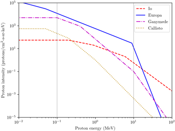
Figure 5. Piecewise continuous fits to the measured proton intensities at the orbits of the Galilean moons. Gray lines at 0.1 and 10 MeV bound the proton energies used to estimate the X-ray flux. Quantitative values for these parameters can be found in Table 3.
Download figure:
Standard image High-resolution imageTable 3.
Best-fit Parameters of the Piecewise Continuous Power-law Model  Fitted to the Proton Energy Distributions
| Energy | Np0 | α | Np |
|---|---|---|---|
| (MeV) | (cm−2 s−1 sr−1 keV−1) | ||
| Io | |||
| 0.1–0.2 | 55.0 | 0 | 55.0 |
| 0.2–0.9 | 1.94 × 10³ | 0.67 |

|
| 0.9–6 | 7.70 × 10⁴ | 1.21 |

|
| 6–10 | 3.78 × 10⁹ | 2.46 |

|
| Europa | |||
| 0.1–9 | 5.46 × 10⁶ | 1.33 |

|
| 9–10 | 9.95 × 1034 | 8.48 |

|
| Ganymede | |||
| 0.1–0.4 | 1.49 × 10⁶ | 1.23 |

|
| 0.4–10 | 2.06 × 10¹⁰ | 2.83 |

|
| Callisto | |||
| 0.1–0.2 | 1.27 × 10⁵ | 1.39 |

|
| 0.2–1 | 1.47 × 10⁸ | 2.72 |

|
| 1–10 | 1.12 × 10¹⁰ | 3.35 |

|
Note. Fits for proton energies in the range 0.1–10 MeV were made to the proton energy distributions measured by Galileo in the vicinity of the Galilean moons.
Download table as: ASCIITypeset image
Combining the PIXE yields and the incident proton intensity using Equation (1), we compute the expected PIXE yields for the five emission lines for the four moons. The results of these calculations are shown in Table 4. For Io, more than an order of magnitude fewer counts were estimated for PIXE than were actually observed by Chandra for the oxygen, sodium, and sulfur lines. Thus, PIXE does not adequately explain the source of the X-rays observed from Io. On the other hand, the observed numbers of counts from Europa in these lines are in reasonable agreement, to within a factor of a few, with the numbers estimated from the NIMS fit composition. A number of PIXE counts were predicted from Ganymede—and indeed, a peak at O was observed in Ganymede's spectrum. On the other hand, Figure 1 reveals that both Io and Ganymede produced X-ray emission in a broad band not accounted for by PIXE. As can be seen from Table 4 and Figure 1, Callisto was only just detected in our X-ray observations, which is consistent with the estimated PIXE fluxes for a surface of half ice (H2O) and half micrometeoroids, but the small numbers of counts observed mean that no definitive conclusions can be drawn.
Table 4. Kα Counts for PIXE from 0.1 to 10 MeV Protons
| Moon | Io | Europa | Ganymede | Callisto | ||||
|---|---|---|---|---|---|---|---|---|
| Observed Chandra counts per 80 ks | ||||||||
| C | ||||||||
| O | 2.5 | 2.0 | 1.25 | 0.5 | ||||
| Na | 0.5 | 0.25 | ||||||
| S | 1.25 | 0.25 | 0.25 | |||||
| K | ||||||||
| Surface | SO2 | SO2 | H2O | NIMS fit | H2O+ | H2O+ | ||
| composition | +1.4% lava | micrometeoroids | micrometeoroids | |||||
| Estimated counts in 80 ks from Chandra | ||||||||
| C | 0.01 | 0.3 | ||||||
| O | 0.04 | 0.04 | 9 | 7 | 2.2 | 0.03 | ||
| Na | 0.1 | |||||||
| S | 0.08 | 0.08 | 0.4 | |||||
| K | 0.01 | |||||||
| Estimated IX (photons cm−2 s−1 sr−1) | ||||||||
| C | 10 | 186 | 3.4 | |||||
| O | 57 | 57 | 16,700 | 13,800 | 1420 | 21 | ||
| Na | 99 | 0.3 | 0.005 | |||||
| S | 107 | 105 | 718 | 2.5 | 0.03 | |||
| K | 21 | 0.01 | ||||||
| Estimated counts in 1 ks from a notional mission 100 Europa radii from the moon | ||||||||
| C | 0.9 | 0.9 | 155 | 155 | 2920 | 54 | ||
| O | 898 | 897 | 262,000 | 216,000 | 22,300 | 326 | ||
| Na | 1.5 | 1.5 | 39 | 1550 | 5 | 0.08 | ||
| S | 1680 | 1650 | 83 | 11,300 | 39 | 0.4 | ||
| K | 1.1 | 1.1 | 120 | 322 | 0.1 | 0.001 | ||
Note. The Observed Chandra counts rows list the observed number of counts per 80 ks; the Chandra estimate is for a ±100 eV band around the emission line in an 80 ks observation with an effective area of 400 cm2, similar to the Chandra effective area in the AO3 observing cycle; IX is the X-ray intensity in the lines predicted for the different surface compositions described in the text using the proton distributions from Table 3; and the notional mission counts are the estimates for a notional instrument with an effective area of 50 cm2 at a distance of 100 Europa radii in a 1 ks observation. If the composition were varied, the estimated counts and X-ray intensities would scale proportionally. For the notional mission estimates in this table, elements not present in the modeled surface compositions have been added at a concentration of 1 ppt by mass and can be used for order-of-magnitude scaling for different compositions or other trace elements. K is present in the surface models for Ganymede and Callisto at a mass fraction of 0.05 ppt, so many fewer counts are estimated than would have been had it been present at the "trace" level of 1 ppt by mass. Bold numbers in the estimated Chandra counts section should be compared with the corresponding bold numbers giving observed counts.
Download table as: ASCIITypeset image
Table 6. X-Ray Fluxes from Electron Bremsstrahlung
| Moon | Observed | Target | Estimated | Estimated |
|---|---|---|---|---|
| Chandra Counts | Matrix | IX | Chandra Counts | |
| Io | 5.4 | SO2 | 1870 | 1.4 |
| Europa | 3.0 | H2O | 15,200 | 8.2 |
| Ganymede | 2.6 | H2O | 8260 | 13 |
| Callisto | 0.4 | H2O | 1260 | 1.6 |
Note. The Observed Chandra counts column lists, in bold, the observed number of counts in the 0.5–5 keV band scaled to 80 ks; the X-ray intensity, IX, is the intensity in the same band in units of photons cm s
s sr−1 predicted from the electron bremsstrahlung model for the target matrix specified and using the electron parameters from Table 5; and the Chandra estimate is the electron bremsstrahlung count estimate, in bold, for an 80 ks observation with an effective area of 400 cm2, similar to the Chandra effective area in the AO3 observing cycle. The counts given in bold are to be compared for the relevant moon.
Download table as: ASCIITypeset image
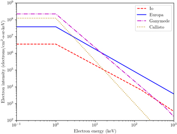
Figure 6. Piecewise continuous fits to the measured electron intensities at the orbits of the Galilean moons. Quantitative values for these parameters can be found in Table 5.
Download figure:
Standard image High-resolution image
Figure 7. Predicted X-ray intensity from electron bremsstrahlung from Europa for incident electrons in different energy ranges using the thick-target bremsstrahlung model of Pella et al. (1985). We include the effects of self-absorption, which has a strong effect on the X-ray flux below 10 keV and for the more penetrating electrons. Dashed lines show what the flux would be without self-absorption.
Download figure:
Standard image High-resolution image
Table 5.
Best-fit Parameters of the Piecewise Continuous Power-law Model  Fitted to the Electron Energy Distributions
| Energy | Ne0 | α | Ne |
|---|---|---|---|
| (keV) | (cm−2 s−1 sr−1 keV−1) | ||
| Io | |||
| 0.1–1 | 3.54 × 10⁶ | 0 | 3.54 × 10⁶ |
| 1–150 | 3.54 × 10⁶ | 1.26 | 3.54 × 10⁶E−1.26 |
| 150–1000 | 1.43 × 10⁷ | 1.54 | 1.43 × 10⁷E−1.54 |
| Europa | |||
| 0.1–1 | 3.80 × 10⁷ | 0 | 3.80 × 10⁷ |
| 1–1000 | 3.80 × 10⁷ | 1.33 | 3.80 × 10⁷E−1.33 |
| Ganymede | |||
| 0.1–1 | 2.22 × 10⁸ | 0 | 2.22 × 10⁸ |
| 1–600 | 2.22 × 10⁸ | 2.00 | 2.22 × 10⁸E−2.00 |
| 600–1000 | 5.25 × 10⁹ | 2.50 | 5.25 × 10⁹E−2.50 |
| Callisto | |||
| 0.1–1 | 1.24 × 10⁸ | 0 | 1.24 × 10⁸ |
| 1–1000 | 1.24 × 10⁸ | 2.54 | 1.24 × 10⁸E−2.54 |
Note. Fits for electron energies in the range 0.1–1000 keV were made to the electron energy distributions measured by Galileo in the vicinity of the Galilean moons.
Download table as: ASCIITypeset image
We note that, while our observations span more than a decade of Chandra observations, we base our X-ray flux estimate on one average measurement of the magnetospheric particle intensity made by Galileo before any of the X-ray observations were made. Differences in the X-ray brightness of the moons between different observations could be due to significant variability in the particle fluxes reaching their surfaces. The modeled X-ray fluxes should therefore be taken only as rough estimates for comparison. The X-ray flux will change proportionally with any variations in the normalization of the proton energy spectrum. The relative strength of the emission lines is not strongly dependent on variations in the power-law index of the proton energy distribution. We recomputed the emission line fluxes using Equation (1), varying the spectral index by 5%. We found 5% variation in the relative fluxes of the S and O lines, but only about 1.5% variation in the relative fluxes of Na and O. Nondetections in some of the observations could easily be accounted for by variations in the energetic proton population.
3.2. Electron Bremsstrahlung
We model the electron bremsstrahlung radiation from the surfaces of Io and Europa using the thick-target model of Pella et al. (1985). As with the PIXE modeling, we assume that the moon is embedded in a uniform cloud of energetic particles—in this case, electrons. We neglect any orbital variation or any differences in emission from the leading and trailing sides of the moon due to compositional differences or the rotation of the Jovian magnetosphere. The X-ray intensity, I(E), is given by

where E0 and E are the incident electron and radiated photon energies, respectively, in keV (with  ), K is a constant (2.20 × 10⁻⁷ photons keV−1(e−)−1 sr−1), and Z is the atomic number of the target material. The electrons are sufficiently energetic that they penetrate deeply into the surface and self-absorption of the material must be included. Parameterization of the self-absorption as a function of target material and electron energy based on laboratory measurements of electron impact X-ray sources is given in Equations (17) and (21) of Pella et al. (1985). Mass absorption coefficients are taken from Henke et al. (1993). Computation of the differential (per unit bandpass) X-ray flux is then determined by integration of the appropriate electron energy distributions. The electron energy distributions below 1 keV were arbitrarily capped at their values at 1 keV. These low-energy electrons make little contribution to the bremsstrahlung output, and this will not affect our conclusions. As with the PIXE calculation, we ignore the effects of limb brightening or darkening.
Note that electron bombardment will also produce X-ray fluorescence at the same lines as the PIXE radiation. Both empirically and based on theory, the line emission from low Z (i.e., Al and lighter) metallic targets in laboratory electron impact sources is typically 10%–20% of the broadband continuum emission (Green & Cosslett 1961; Sulkanen et al. 1995). For higher Z elements (e.g., S), the line emission will contribute a relatively larger fraction of the overall flux—up to as much as 50%. This contribution will depend in detail on the electron energy distribution and self-absorption in the target—and most critically, the precise elemental composition of the target. The X-ray flux from electron impact will be dominated by continuum emission for icy moons like Europa (i.e., mostly low-Z material), and will be at least half the emission from rocky moons like Io (i.e., higher-Z materials like S). Thus, for simplicity, we do not include line emission in our spectral models.
One complication we must address is that the model of Pella et al. (1985) is for targets of a single element, whereas the surfaces of the moons are, in general, made up of a variety of different elements. Markowicz & Van Grieken (1984) solve this problem by finding an effective atomic number, which we are calling ZMVG, to predict the generated bremsstrahlung background intensity in electron-probe X-ray microanalysis of a compound, or any material of more than a single element. This effective atomic number is given by

where wi is the mass fraction of element i, Zi its atomic number, and Ai its atomic weight. If ni is the number of atoms of element i in one molecule, or one unit, of the target matrix, and  the total number of atoms in one unit, then the atomic fraction of element i,
  . Now the molecular weight of the material
  , and the mass fraction of element i,
  , so
, so  . Thus,

This shows that  is a function of only atomic numbers and the atomic fractions. In this work,
  was used in estimating the X-ray emission from electron bremsstrahlung for surfaces of more than one element. The surface is assumed to be SO2 (
 ) for Io, the NIMS fit composition as described for the PIXE modeling (ZMVG = 8.4) for Europa, and O (Z = 8) for the other icy moons.
The effect of self-absorption is significant below photon energies of 10 keV, reducing the flux by almost an order of magnitude from the unabsorbed estimate. The most energetic electrons penetrate the deepest, and once they go below a few optical depths of a photon of a given energy, the photons generated beyond that depth do not escape. As with PIXE, the X-ray emission occurs in a thin layer at the surface of the ice, typically a few microns to tens of microns. The depth of this layer varies with the escaping photon energy.
Near Io, Galileo measured the ion energy distribution while both Galileo and Voyager 1 sampled the electron energy distribution (Paranicas et al. 2003). We used a piecewise continuous power law fitted to the Galileo data to model the electron distribution at Io. Likewise, the differential electron energy distribution at the icy Galilean moons was modeled as piecewise continuous power laws fitted to Galileo's measurements in their environs (Cooper et al. 2001). Parameter values for the electron energy distributions are given in Table 5 and plotted in Figure 6. The X-ray intensities at the surface of Europa derived using these electron energy distributions are plotted in Figure 7. We compute estimated fluxes seen by Chandra by integrating these intensities over the 0.5–5.0 keV band and assuming an effective area of 400 cm2 for the instrument independent of energy (a good approximation early in the mission), an observation time of 80 ks, and a distance from Earth of dEarth = 4.5 au. We predict ∼1.4 and ∼8.2 counts from Io and Europa, respectively, in an 80 ks observation. These values are included in Table 6 for comparison with the PIXE predictions in Table 4 and the observed data.
4. Interpretation
Several conclusions can be drawn from comparison of the observed and modeled X-ray fluxes from Io and Europa. First, the emission from Europa is reasonably well-described by both the PIXE and electron bremsstrahlung processes. The observed flux in the O line is within a factor of a few of the predicted strength for the PIXE model, and the total rate in the electron bremsstrahlung model is roughly consistent with predictions. Given the uncertainties in both the modeling and the particle environment at the time of the observations, we should only expect the result to be accurate to within a factor of a few. In fact, the measurement is consistent given the errors on the particle spectrum quoted in Cooper et al. (2001). We can also make no definitive statement about the X-ray spectrum, given the relatively low number of counts in the existing data. This issue could be resolved with a deep (several Ms) Chandra observation and a detection or strong upper limit in the 2–7 keV band. The PIXE model predicts no X-ray flux in this band, whereas there should be detectable continuum emission in this band if electron bremsstrahlung dominates.
For Io, on the other hand, the observed X-ray flux in the 0.5–5.0 keV band significantly exceeds (by roughly two orders of magnitude) that predicted by PIXE. The observed strength of the S line is a factor of ∼20 greater than the PIXE prediction, and the relative strength of the O line is even greater, but the other lines should be undetectable if PIXE is the dominant emission process. In particular, the PIXE model cannot explain the broadband flux seen by Chandra. Note that the differences in predicted PIXE flux from Io and Europa are consistent with the significant difference in the normalizations in the curves of particle distributions shown in Figure 5. Even though there are emission peaks at S and O, the photons are more uniformly distributed across the band, suggesting a continuum process. The flux predicted by the electron bremsstrahlung model for Io is only a factor of a few smaller than the observed flux, and well within the uncertainties of the normalization of the particle distribution. We therefore conclude that the X-ray emission from Io can be plausibly attributed to electron bremsstrahlung. Bear in mind that the peaks at O and S are entirely in accord with this interpretation, as electron impact will also create characteristic fluorescence, which we did not include in our model. Nevertheless, the continuum photons will remain a dominant feature of the overall flux.
Finally, for realistic assumptions about the elemental surface composition, we computed the predicted X-ray fluxes from Ganymede and Callisto using both the PIXE and electron bremsstrahlung models as shown in Tables 4 and 6. Chandra ACIS observations for Ganymede show a peak around the O Kα line as well as a broad continuum that can be attributed to electron bremsstrahlung. The presence of a continuum suggests that some electrons are precipitating to the surface. Because of Ganymede's magnetic field, these will probably be at higher latitudes.
The predicted PIXE flux from Callisto would not be detectable, while the X-ray emission from Callisto due to electron bremsstrahlung would be barely detectable with Chandra ACIS. Most of the few events observed with ACIS are near the O line, but Callisto is too faint to draw any conclusions about the origin of this emission.
We have also reanalyzed 15 Chandra HRC observations of the Galilean moons, looking at events in the same areas around the moons as described for the ACIS observations. These HRC observations are Obs IDs 1862, 2519, 15669, 15670, 15671, 15672, 16299, 16300, 18301, 18608, 18609, 20000, 20001, 20002, and 20733. The HRC is able to detect X-rays nominally between 0.07 and 10 keV, but without the spectral resolution of ACIS. Also, much higher background levels are found because the HRC is not as capable as ACIS at rejecting spurious background events due to high-energy particles. Indeed, most of the events detected in the collecting areas for the moons are background events. These results are shown in Table 7. A weak detection of X-ray emission from Ganymede was made. The sensitivity of the HRC at the oxygen line (525 eV), where the greatest number of counts occurs in ACIS, is a factor of a few less than ACIS early in the mission. The instrumental background in the HRC is also more than an order of magnitude larger than in ACIS. Early in the mission, ACIS was considerably more sensitive than HRC for photon energies E < 1 keV. Contamination has built up on ACIS during the course of the mission, however, progressively degrading its low-energy response (Plucinsky et al. 2018). The sensitivity of the HRC to neutral O fluorescence is now more than an order of magnitude better than ACIS, and is why we coadded all the recent HRC observations.
Table 7. HRC Observations of the Galilean Moons
| teff | S: Counts | Counts in | B: Scaled | S − B: | |||
|---|---|---|---|---|---|---|---|
| (s) | in Moon | Background | Background | Counts | σ |

|
|
| Moon | Area | Area | Counts | ||||
| Io | 584,880 | 123 | 314 | 104.7 | 18.3 | 12.6 | 1.5 |
| Europa | 643,440 | 90 | 236 | 78.7 | 11.3 | 10.8 | 1.1 |
| Ganymede | 654,180 | 241 | 603 | 201.0 | 40.0 | 17.5 | 2.3 |
| Callisto | 669,060 | 192 | 535 | 178.3 | 13.7 | 15.9 | 0.9 |
Note. The observation times, teff, are given after removing transits of the Jovian disk. The background area is three times the area over which counts for the moon were collected. Here,  , in bold, is the net number of counts detected, σ is the calculated error in
  , and (S − B)/σ, also in bold, is given to allow judgment of the significance of the detection for each moon.
Download table as: ASCIITypeset image
5. Implications and Conclusions
We reanalyzed all existing archival CXO observations of the Galilean moons. In addition to confirming the detections of Io and Europa first reported by Elsner et al. (2002), X-ray emission was also detected from Ganymede and marginally from Callisto. We computed the X-ray spectrum of each of the Galilean satellites using two models—PIXE and electron bremsstrahlung—for the particle fluxes derived from the Galileo mission. We find that the X-ray emission from Io and Ganymede can be plausibly attributed to electron bremsstrahlung, and the X-ray emission from Europa could be due to either PIXE or electron bremsstrahlung. No conclusion can be drawn about the origin of the faint X-ray spectrum of Callisto. It will not be feasible to detect emission from weaker lines with the current generation of Earth-orbiting X-ray observatories in any reasonable observing time without a significant increase in the density of nonthermal particles in the Jovian magnetosphere. The next generation of X-ray observatories, such as Athena (Nandra et al. 2013) and Lynx (Gaskin et al. 2018), will have an order of magnitude more effective area and will include high spectral resolution X-ray calorimeters. With very little effort, these observatories should be able to confirm our results on Io, Europa, and Ganymede, and make a firm detection or place a strong upper limit on the X-ray flux from Callisto. These instruments will have the sensitivity and spectral resolution to detect emission from all of the dominant species, and potentially some of the less abundant elements as well.
The primary goal of our work has been to use the observed X-ray flux from the Galilean moons to determine something about their composition and the nature of their interactions with the nonthermal particles of the Jovian magnetosphere. However, an Earth-orbiting X-ray telescope with much larger effective area than Chandra or XMM-Newton could, in principle, be used to monitor variations in the energetic electron and proton populations of the magnetosphere. Simple changes in the density of the particles would be tracked by changes in the X-ray flux from the Galilean moons, and variations in the energy spectral index of the energetic particles would be exhibited by changes in the observed line ratios (for PIXE) or the shape of the bremsstrahlung continuum (for electron precipitation).
Finally, we would like to highlight that the science return from an X-ray spectrometer on a mission to any of the Galilean moons, but particularly Europa, on either an orbiter or lander, would be substantial. Due to proximity alone, the flux would be 6–7 orders of magnitude larger, such that the presence of trace elements in small concentrations could easily be measured in short exposure times. Even in the presence of the considerable detector background, this instrument could measure the presence of an element such as Na, Mg, or Cl in the surface of Europa to a level of 1 ppt by mass in about 15 minutes. A dedicated instrument on a lander could make abundance measurements to a few tens of ppm in longer integration times (Tremblay et al. 2018). Such an instrument on an orbiter could map the elemental abundance across the surface. If the instrument included an X-ray optic, it could potentially map variations in the elemental surface composition to scales as small as tens of meters depending on proximity. Such an instrument on a lander could make elemental abundance measurements on scales of less than meters.
Archived data were obtained from the Chandra Data Archive (https://cda.harvard.edu/chaser/) and X-ray emission from the moons was selected using the JPL Horizons web interface (https://ssd.jpl.nasa.gov/horizons.cgi) to determine their positions. John (Iain) L. Campbell from the University of Guelph kindly supplied the GUYLS program from the GUPIX package (http://pixe.physics.uoguelph.ca/gupix). This enabled us to calculate the X-ray fluorescence that would be produced by proton impact on a surface of known composition. This work was supported by NASA contracts NAS8-03060 and AR6-17001X and SI Scholarly Studies Sprague Grant 488100. We thank the anonymous referee for detailed comments that significantly improved this paper.