


Abstract
In situ measurements at heliospheric shocks show that inside the shock front large-scale electric and magnetic fields are accompanied with strong small-scale fields. Until recently, it was widely believed that particle dynamics is determined by the large-scale fields. During the last several years, claims have been made that the small-scale fields are of primary importance. Here we show that the large-scale fields govern the ion motion while both large- and small-scale fields are important for electrons.
Export citation and abstract BibTeX RIS
1. Introduction
Collsionless shocks are among the most efficient accelerators of charged particles in the universe (Blandford & Eichler 1987; Giacalone 2003). The diffusive particle acceleration, which occurs at large scales, is nevertheless closely related to the processes occurring in the shock front (Drury 1983). In situ observations of shocks, necessary for studies of the shock structure, are possible only in the heliosphere (Bale et al. 2005; Burgess et al. 2005; Krasnoselskikh et al. 2013). The standard magnetohydrodynamical representation of a collisionless shock is a planar discontinuity through which a plasma flow is decelerated (de Hoffmann & Teller 1950). The plasma and the field states on both sides are related through conservation laws and jump conditions for electromagnetic fields, altogether known as Rankine–Hugoniot relations (Kennel et al. 1985; Kennel 1988). Real shocks have finite widths. It was realized quite early that the magnetic structure in the transition region becomes nonmonotonic with the increase of the Mach number (Greenstadt et al. 1975, 1980; Livesey et al. 1982; Russell et al. 1982a, 1982b; Mellott & Greenstadt 1984; Scudder et al. 1986; Farris et al. 1993; Newbury & Russell 1996; Newbury et al. 1997, 1998; Hobara et al. 2010). The width of the sharpest transition (the shock ramp) is typically comparable with the ion inertial length Li = c/ωpi,  in low-Mach number shocks (Farris et al. 1993). A ramp is a fraction of the ion inertial length in high-Mach number shocks (Newbury et al. 1998; Hobara et al. 2010), and can sometimes be as small as the electron inertial length Le = c/ωpe (Newbury & Russell 1996; Hobara et al. 2010). It was also realized that a cross-shock electrostatic electric field should be present that decelerates ions (Woods 1969; Morse 1973; Sanderson 1976). It was widely believed that the cross-shock potential has a smooth monotonic profile of the same scale as the magnetic ramp (Goodrich & Scudder 1984; Scudder 1995). Accordingly, the electron dynamics in the shock front was suggested to be governed by this macroscopic potential (Feldman et al. 1982; Schwartz et al. 1988; Gedalin & Griv 1999; Hull et al. 2001). However, observations have shown electric field spikes of substantially smaller scales (Wygant et al. 1987; Walker et al. 2004; Hobara et al. 2010). It was suggested that small-scale electric fields can energize electrons nonadiabatically (Balikhin et al. 1993). It was also predicted that even-smaller-scale electric fields should be present inside the shock due to electron streaming instabilities (Gedalin 1999). Recent observations have revealed strong small-scale electric fields inside the shock front (Wilson et al. 2014a, 2014b; Goodrich et al. 2018, 2019; Vasko et al. 2018; Cohen et al. 2019; Wang et al. 2020). Such fields should affect the electron motion. Some works even speculate that ions may be affected (Goodrich et al. 2019; Wang et al. 2020). The observed fields are highly variable. It is even sometimes claimed that no nonzero integrated cross-shock potential
  exists and ion deceleration is done by the oscillating fields. In parallel, ubiquitous large-amplitude whistlers have been observed even at low-Mach number shocks (Wilson et al. 2009, 2012, 2017). Although it has been analytically shown that the magnetic deflection is weak even at the ramp crossing (Gedalin 1996a, 1996b, 1997a, 1997b), it is still sometimes claimed that whistler precursors are of primary importance in the formation of ion distributions inside the shock front. In this paper we analyze the possible influence of the abovementioned fields on the particle motion, focusing on the effects of small-scale electrostatic spiky fields. The paper is organized as follows. In Section 2 we analytically determine the conditions of the perturbative approach in ion dynamics. In Section 3 we numerically trace ions in a model shock front with the strong small-scale electrostatic fields included. In Section 4 we extend the analysis to electron tracing in the same shock.
2. Basic Theory
The problem allows for a general formulation as a perturbation of a motion in mean background fields. However, for our purposes a simple analysis will be more transparent. Let


where Bx, Bz, and Ey are constants and  are unity vectors in the directions of the axes. The equations of motion of an ion are

Let  ,
,  , where


Here  . In the absence of perturbations ions are assumed to drift with the velocity
  , so that
 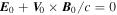 . Let
. Let

The equations of motion take the form


where  and Ω = qB0/mc. The solution is


where we replaced t = x/V0 from the zeroth order.
The perturbed fields are assumed to be a series of spikes of both polarities so that the means vanish, that is,  and
and  , where the integration is along the whole unperturbed path. In what follows we are interested in the change in the ion velocity upon crossing a spike of one polarity. Let L be a typical spatial scale of the spike such that ΩL/V0 ≪ 1. Then the change of the ion velocity upon crossing a spike is
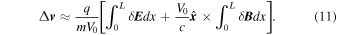
Now a simple estimate gives

where E0 = V0B0/c and δE and δB are mean values that are below the maximum values of the perturbations. The applied perturbative approach is justified if Δv/V0 ≪ 1. For an electromagnetic whistler of L≲c/ωpi and δB/B0 ≲ 1 one has

where M = V0/VA is the Alfvenic Mach number. Here VA = cΩ/ωpi.
For an electrostatic spike of L ≲ c/ωpe one has

and to achieve any substantial effect one needs 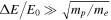 .
.
In a more general way, let small-scale zero mean variations be superimposed on slowly varying background fields. Then the velocity of an ion can be represented as a slowly varying mean and quickly varying perturbations. The cumulative effect of the perturbations along the path of the ion would vanish in the first order on the single spike  and only the effect of the varying background would remain. Goncharov et al. (2014) and Wilson et al. (2017) argue that whistler precursors may play important roles in the redistribution of the energy of the bulk flow. In their analysis they miss the gradually increasing mean magnetic field, which is observed in the precursor region. Goodrich et al. (2018) mention solar wind deceleration in the absence of whistler wavepackets as surprising, yet in both regions the background magnetic field gradually increases as can be seen in their Figure 3. It is also claimed that small-scale variations (down to the Debye length; Goodrich et al. 2018, 2019; Wang et al. 2020) can decelerate ion flow. Noticeable deceleration would require electric fields of at least an order of magnitude higher.
3. Numerical Analysis of Ion Motion
In case the equations are not sufficiently convincing, we illustrate the analysis by direct numerical tracing of ions in a model shock profile with superimposed large-amplitude small-scale electrostatic fields. A similar numerical analysis of whistlers will be presented elsewhere. The analysis is done in the normal incidence frame where the upstream plasma velocity is along the shock normal. The electric field used in the analysis is shown in Figure 1.

Figure 1. Top panel: superposition of a strong small-scale electric field and a weak slowly varying cross-shock field, Ex/Eu,  . Bottom panel: the accumulated cross-shock potential
  ,
,  .
.
Download figure:
Standard image High-resolution imageThe cross-shock electrostatic electric field Ex is a superposition of a series of large-amplitude small-scale bipolar spikes of zero mean and a slowly varying single peak field. The corresponding cross-shock potential is a superposition of a monotonically increasing envelope and series of spikes. The angle between the shock normal and the upstream magnetic field is θ = 70°. The upstream motional electric field is  . The electric field in the figure is normalized on Eu. The potential
  is normalized to the upstream ion energy,
  . The overall normalized cross-shock potential is ϕmax = 0.4. The small-scale field is grossly exaggerated, the chosen amplitudes are much larger than the measured amplitudes, and the single spike potential ϕsingle ≈ 0.1 by far exceeds the observed values (Goodrich et al. 2018, 2019; Vasko et al. 2018; Cohen et al. 2019; Wang et al. 2020). The slowly varying potential follows the magnetic profile. In the present analysis the magnetic compression is Bd/Bu = 2.3 and the Alfvenic Mach number is M = 2.2. For small
  the ratio of the upstream ion thermal speed
  to the upstream speed Vu is
 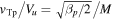 and is also small. Motion of an incident ion that has the upstream plasma velocity is representative in this case. Figure 2 shows the velocity of a cold ion beam, vx(x), for four cases: (a) no electric field at all, (b) no weak slowly varying field, only large-amplitude small-scale field, (c) no large-amplitude small-scale field, only weak slowly varying field, and (d) both fields. For cases (a) and (b), as well as for (c) and (d), the velocities are identical except small-scale fluctuations in the region of spikes. This means that the small-scale spikes cause only fast fluctuations of the amplitude determined by the cross-spike potential. The curves for no cross-shock potential show no deceleration within the ramp. Deceleration begins in the downstream region due to the gyration. The curves with the cross-shock potential show clear deceleration within the ramp. Such deceleration is necessary for the magnetic field increase, since the magnetic pressure increases at the expense of the dynamical pressure which is simply
  in this case. Momentum conservation requires

and, accordingly

The bottom line is that zero-mean large-amplitude small-scale electric fields are not able to decelerate the ion flow, contrary to claimed by Goodrich et al. (2018, 2019). A nonzero  is absolutely necessary.

Figure 2. Normalized component of the velocity of a cold ion beam along the shock normal, vx/Vu, as a function of the coordinate. The magnetic profile is shown in black. Two blue lines correspond to the cases without the slowly varying fields, that is,  . Two red lines are for ϕmax = 0.4. The small-scale field adds only small-scale fluctuations of the velocity.
Download figure:
Standard image High-resolution image4. Effect on Electron Motion
For electrons the above perturbative approach is not valid. For numerical tracing a lower amplitude would be more appropriate. The chosen profile is shown in Figure 3.

Figure 3. Top panel: superposition of a strong small-scale electric field and a weak slowly varying cross-shock field, Ex/Eu,  . Bottom panel: the accumulated cross-shock potential
  ,
,  .
.
Download figure:
Standard image High-resolution imageFigure 4 shows vx versus x for an electron that was initially drifting toward the shock.
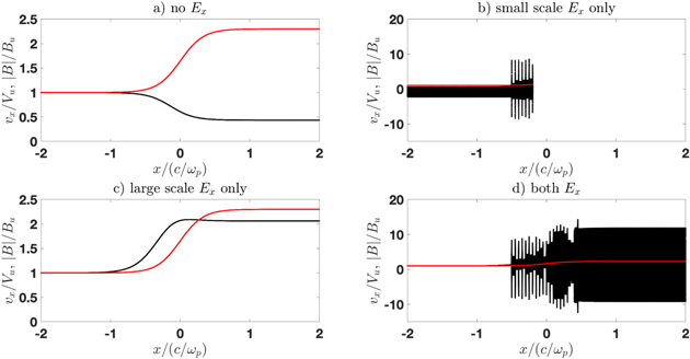
Figure 4. Tracing of an electron with initial  : (a) no Ex, (b) only small-scale Ex, (c) only large-scale Ex, and (d) both fields.
Download figure:
Standard image High-resolution imagePanel (a) shows the electron velocity vx evolution across the shock for the case when there is no cross-shock electric field Ex at all. As expected, the electron velocity adiabatically reduces to the downstream drift velocity. Panel (b) shows the electron behavior when only small-scale Ex is present inside the ramp. The electron is reflected and does not cross the shock. Panel (c) shows the electron behavior when only large-scale Ex is present. The motion is adiabatic and the electron does not begin to gyrate. The acceleration is due to the electric field parallel to the ambient magnetic field. Panel (d) shows the evolution of the electron velocity when both small-scale and large-scale fields are present. As a result, the electron begins to gyrate.
For electrons the ratio  is not necessarily small even for low βe. Thus, the single trajectory does not represent all or most of the electrons. Figure 5 shows orbits of 40 electrons taken randomly from the initial Maxwellian distribution with βe = 0.05. Overall, there are 4000 particles in the distribution. Of these, 3308 are moving initially toward the shock front, of which 183 (5.5%) are reflected.

Figure 5. Orbits vx(x) of 40 electrons taken randomly from a Maxwellian distribution with  . Both fields are present in the ramp.
Download figure:
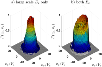
Standard image High-resolution imageFigure 6 shows the projection of the downstream distribution on the vx − vy plane:  . The projected distribution function is normalized. The incident Maxwellian distribution of electrons consists of 20,000 particles with βe = 0.05. Only those moving toward the shock are traced. The projection shows the electrons crossing the shock just behind the ramp, within 0.5 < x/(Vu/Ωu) < 0.6. The left panel shows the projected distribution in the case where only the large-scale Ex is present inside the ramp. The shape corresponds to the expected adiabatic perpendicular heating. The right panel shows the projected distribution in the case where both large-scale and small-scale Ex are present inside the ramp. The perpendicular heating is stronger and shows clear deformation toward the observed flat-top shape (Feldman et al. 1982).
Figure 6. Projection of the normalized downstream distribution just behind the ramp. Left panel: large-scale field Ex only. Right panel: both Ex.
Download figure:
Standard image High-resolution image
5. Discussion and Conclusions
In the above analysis of the ion motion in small-scale structures it is essential that the interaction of the field with the particles is nonresonant, that is, the time of interaction with a single structure is a small fraction of the ion gyroperiod. For interaction to be resonant the field should be slowly varying in the particle rest frame. In the shock frame this means that the velocity of the structure is nearly equal to the velocity of the ion. For the bulk flow that would mean that the observed electric fields are standing in the flow. In this case only ions that incidentally are in the same place as the small-scale structure, would be affected. At present, there is no observational evidence that the observed electrostatic fields drift with the flow. If the velocity of a structure relative to the flow is not substantially smaller than Vu, there still may exist ions in the tail of the distribution that might be resonant with the fields (Wilson et al. 2014b; Wang et al. 2020). The number of these ions is small unless the upstream βp is large. Some reflected ions may also occasionally appear resonant with the small-scale fields. Dissipation due to this interaction occurs after the primary energy redistribution has already occurred, in the form of ion reflection, and therefore is not essential for the shock maintenance. In summary, deceleration of the bulk ion flow and conversion of the directed flow energy into other forms requires substantial nonzero net potential jump  across the shock ramp. The field Ex may be strongly inhomogeneous and the corresponding potential does not have to increase monotonically. If
  ions cannot be decelerated and the momentum cannot be transferred to the magnetic field as required for the magnetic field increase at the ramp. This theoretical statement is confirmed by observations (Walker et al. 2004; Dimmock et al. 2012; Goodrich et al. 2018).
The electron mass is about 2000 times smaller as well as the corresponding gyroperiod. For Te = Tp the electron gyroradius is smaller by a factor of  . Therefore, the small-scale structures can strongly affect the electron motion. As is shown above, the presence of electric spikes inside the ramp may cause electron reflection. Electron heating inside the shock may occur as a series of short regions of strong nonadiabatic energization in the direction perpendicular to the magnetic field, intermittent with the regions where electrons are adiabatically accelerated along the magnetic field. If small-scale fields are absent, electrons are only accelerated along the magnetic field.
For ions, the results are conclusive and the necessity of a nonzero net cross-shock potential is firmly established and does not depend on a specific shape of the electric field inside the shock transition. For electrons, the above results are illustrative and only indicate possible effects, since the field structure is important. Further studies are needed to quantify the electron dynamics inside the ramp.
The author is grateful to L. Wilson for the discussions that triggered this study. Nonadiabatic electron heating in thin layers was suggested to the author by V. Krasnoselskikh in 1995 but was not explored until now.