


Abstract
There are indications that the perpendicular transport of energetic particles is sometimes subdiffusive for intermediate timescales. This corresponds to a scenario where particles follow diffusive magnetic field lines while they also move diffusively in the parallel direction. This type of transport should occur at times after the ballistic regime but before the particles experience the transverse complexity of the turbulence. In this article we present a detailed analytical investigation of distribution functions of particles experiencing compound subdiffusion. Simple approximations of particle distributions are derived which can easily be used in applications. We also compare our findings with test-particle simulations performed for slab turbulence corresponding to the case of vanishing transverse turbulence structure.
Export citation and abstract BibTeX RIS
1. Introduction
The understanding of the motion of electrically charged and energetic particles propagating through a magnetized plasma is a fundamental problem of theoretical astrophysics and space science. Examples are the propagation of cosmic rays through interplanetary and interstellar spaces. Due to turbulent electric and magnetic fields, particles experience different scattering mechanisms such as diffusion along and across the mean magnetic field, adiabatic focusing, and stochastic acceleration (see, e.g., Schlickeiser 2002 and Zank 2014 for reviews). In particular diffusion across the mean magnetic field, also simply called perpendicular diffusion, is difficult to understand (see, e.g., Shalchi 2009 for a review). The famous work of Rechester & Rosenbluth (1978) explained the basic mechanisms of perpendicular transport but this was done in the context of laboratory plasmas where Coulomb collisions play a significant role.
In astrophysics collisions are assumed to be less relevant but particles experience strong pitch-angle scattering leading to a diffusive parallel motion. Quantitative theories to solve this problem have been developed. Noticeable steps in the development of such theories are the nonlinear guiding center theory (see Matthaeus et al. 2003), the unified nonlinear transport theory (see Shalchi 2010, 2015), and its time-dependent version (see Shalchi 2017 and Lasuik & Shalchi 2017). In particular the latter theory provides some important insight into the mechanisms of perpendicular transport. The time-dependent theory predicts that subdiffusive perpendicular transport persists in some cases for a long time before normal diffusion is restored. The recovery of diffusion is entirely caused by transverse complexity of magnetic turbulence becoming important. These ideas lead to a heuristic description of perpendicular transport (see Shalchi 2019) similar to the paper by Rechester & Rosenbluth (1978) but for the collisionless case important in astrophysics.
In the subdiffusive regime described above, transverse complexity is not yet important and the particle follows a single magnetic field line. While the particles are tied to diffusive field lines, they experience parallel diffusion due to pitch-angle scattering. As a consequence perpendicular transport is suppressed to a subdiffusive level. This type of transport, which is usually called compound subdiffusion, and the recovery of diffusion due to transverse complexity, was also found numerically via test-particle simulations (see, e.g., Qin et al. 2002a, 2002b).
A discussion of compound subdiffusion was presented in several papers such as Kóta & Jokipii (2000) or later in Shalchi & Kourakis (2007). A more general exploration of subdiffusion, mostly based on numerical work, was performed in Pommois et al. (1999, 2005, 2007) and Zimbardo et al. (2006, 2012). The most comprehensive analytical description of compound subdiffusion was presented in Webb et al. (2006) where not just mean square displacements of particle orbits were determined but also the entire perpendicular distribution function. The work of Webb et al. (2006), which is based on the so-called Chapman–Kolmogorov equation, provides the basis for the work presented in the current paper.
There are several aims we would like to achieve with the current article. The most important are:
- 1.We perform an evaluation of distribution functions and the associated moments entirely based on Fourier transforms. This allows for a very systematic computation of fundamental quantities such as characteristic functions.
- 2.Exact results for the distribution function contain complicated special functions. We present simple analytical approximations which will be useful for applications.
- 3.We provide a comparison of analytical results with test-particle simulations to check the validity of the Chapman–Kolmogorov approach.
The organization of the reminder of this article is as follows. In Section 2 we discuss the Chapman–Kolmogorov equation and some fundamental properties of perpendicular distribution functions of particles experiencing compound subdiffusion. In Section 3 we present some exact results and in Section 4 we employ approximations leading to simplified analytical forms which will be useful for applications. In Section 5 we compare our findings with test-particle simulations and in Section 6 we summarize and conclude.
2. Fundamental Relations
2.1. The Chapman–Kolmogorov Equation
A comprehensive description of compound subdiffusion was presented in Webb et al. (2006). The latter authors employed an approach based on the so-called Chapman–Kolmogorov equation (see, e.g., Gardiner 1985)

where the particle distribution in the perpendicular direction  is given as the convolution integral of the parallel distribution function
  and the field line distribution function
  . This means that particles are assumed to follow field lines and their statistics in the perpendicular direction is entirely controlled by parallel transport and the random walk of magnetic field lines.
All three distribution functions used in Equation (1) can be expressed by a Fourier representation so that
where the last two integrals cover the whole wave number space in x- and y-directions. Based on Equation (1), we find for the Fourier transform of the perpendicular distribution function
This is evaluated for certain parallel transport and field line random walk models below.
2.2. Initial Conditions
It is also crucial to think about initial conditions. First we derive from the third line of Equation (2)

and assume

so that

where we have used (see, e.g., Zwillinger 2012)

twice. This means that any obtained distribution function needs to satisfy the constraint given by Equation (5). Only then the correct initial condition given by Equation (6) is satisfied.
2.3. Moments and Normalization
The nth moment of a distribution is defined via

Due to symmetry we find  if n is odd. Thus, we focus on the case of even n. In order to rewrite this we follow Shalchi & Gammon (2019) and perform the following steps starting by combining Equation (8) with the third line of Equation (2)
where we have used Equation (7) and integration by parts n times. Equation (9) can be used for n = 0 to obtain the normalization condition

Any type of distribution function considered in the current article needs to satisfy this condition as well as the initial condition (5).
2.4. Fourier Transforms and Characteristic Functions
It is important to understand the relation between characteristic functions and Fourier transforms of distribution functions. First we note that the characteristic function is defined via

where the integer number n denotes the dimensionality of the problem. Comparing this with the inverse Fourier transform

yields

Please note that here we assumed that all distribution functions are symmetric in the spectrum

According to Equation (13), characteristic functions and Fourier transforms are directly proportional. The knowledge of characteristic functions is essential for the development of analytical theories for perpendicular diffusion (see, e.g., Lasuik & Shalchi 2017, 2018; Shalchi 2017).
2.5. The Axisymmetric Case
For the axisymmetric case the perpendicular particle distribution function in configuration space can be written as
where we switched from Cartesian to polar coordinates by using
In order to evaluate this further, we can employ

However, the resulting distribution function in Equation (15) must not depend on the angle Φ due to symmetry. Therefore, we can set  so that

where we have used Bessel functions of first kind Jn and the so-called Jacobi–Anger expansion (see, e.g., Cuyt et al. 2008). If we integrate the exponential factor given by Equation (18) over Ψ, we can employ

so that

Using this in Equation (15) yields

which will be used later in this article when specific forms of the function  are considered. Furthermore, we can also compute the distribution function projected onto the x-axis defined via

Using the third line of Equation (2) therein yields
The same result can be obtained if the projection on the y-axis is considered due to symmetry. So far we discussed some general relations. In order to obtain concrete results, we have to specify field line and parallel distribution functions. This is done in the next section.
3. Exact Results
In the following we present some exact results. The corresponding calculations are entirely based on Fourier transforms.
3.1. Characteristic Functions
If the field line random walk is diffusive and assuming a Gaussian distribution of field lines, the field line distribution function is given by

In this case the Fourier transform of the field line distribution function is

The characteristic function, on the other hand, is given by

Thus we find for the perpendicular particle distribution function given by Equation (3)
Using

yields
If we also assume that parallel transport is diffusive and if we employ a Gaussian particle distribution function
we obtain

yielding the characteristic function

Thus, Equation (29) turns into
The occurring integral can be solved by (see, e.g., Gradshteyn & Ryzhik 2000)

where we have used the complementary error function. Finally we obtain

where we have used

Equation (35) is in agreement with Equation (B5) of Webb et al. (2006). Furthermore, we can easily understand that the characteristic function in the perpendicular direction is now given by

Typically, if particle transport is diffusive, we would expect a Gaussian distribution such as the characteristic functions given by Equations (26) and (32). Clearly this is not obtained for compound subdiffusive transport. Note that the scaled complementary error function is defined via

Thus, we can simply write

as well as

These forms are in particular useful for a numerical evaluation in order to avoid arithmetic underflow.
3.2. Distribution Functions in Configuration Space
In order to determine the distribution function in configuration space we can use different approaches. One way of performing this task is to assume Gaussian distributions of field lines and particles in the parallel direction. Using Equations (24) and (30) in (1) yields
After the integral transformation λ = z/ , this becomes
Apart from the variable ρ itself, the distribution function depends only on one single parameter and this is  . The remaining integral can be expressed via the Meijer G-function (see, e.g., Gradshteyn & Ryzhik 2000)
so that
For the projected function we can use
After using again the integral transformation  this becomes
The remaining integral can be expressed via generalized hypergeometric functions (see, e.g., Gradshteyn & Ryzhik 2000)
Using this in Equation (46) allows us to write
Problematic here is that we found solutions depending on more complicated special functions such as the Meijer G-function and generalized hypergeometric functions.
Alternatively, the perpendicular particle distribution function in configuration space is given by Equation (21). With Equation (35) this becomes

which is in agreement with Equation (3.26) of Webb et al. (2006). The projected distribution function is given by Equation (23). For our case this becomes

However, Equations (49) and (50) are difficult to evaluate without employing approximations. Besides a numerical evaluation one can employ different approximations which is done in Section 3. At this point we only compute the values of these two functions at the origin. For x = 0, Equation (50) simplifies to (see, e.g., Gradshteyn & Ryzhik 2000)
Employing (see, e.g., Abramowitz & Stegun 1974)

allows us to write this as

According to Abramowitz & Stegun (1974) we have  so that

Although this formula only provides the value at the origin, it is useful because it is exact. For  , on the other hand, Equation (49) turns into

which does not converge due to the behavior of the integrand at large k⊥. Therefore,  .
.
3.3. Exact Moments
One can easily show that solution (35) satisfies the normalization condition (10). Furthermore, by combining Equation (35) with (9) for n = 2, we can compute the second moment. The second derivative can be written as

Since  and we set
  in Equation (9), the first term goes to zero. In the second term we can use Equation (36) to obtain

so that
Using (see, e.g., Abramowitz & Stegun 1974)

and Equation (35) yields
Using this in Equation (58) provides us with

The latter formula is well-known and was derived in several previous papers (see, e.g., Kóta & Jokipii 2000). A time-dependent or running diffusion coefficient can be defined via

which becomes for the mean square displacement given by Equation (61)

Very clearly we find a declining diffusion coefficient corresponding to subdiffusion. This type of behavior can also be observed in simulations (see, e.g., Qin et al. 2002a). We can also compute the fourth moment. In order to do this we need the following derivatives
and
In the limit  the only nonvanishing derivative of ξ with respect to k⊥ is the one given by Equation (57). This means that all terms except the fourth one on the right-hand side of Equation (65) vanish. Thus, we find

Furthermore, we find with the help of Equation (59)
and, thus,

where we have used  . Combining these findings with Equation (9) yields
Note that this result is in perfect agreement with Equation (2.24) of Webb et al. (2006). A general formula for the nth moment is derived in Appendix A. By using two different methods, it is shown that

for even n. For odd n we have  as mentioned before.
3.4. Transport Equations
The exact relations derived so far were based on the Chapman–Kolmogorov approach as given by Equation (1). Naturally, the following question arises: what is the corresponding transport equation? In the Fourier space a usual diffusion equation for the axisymmetric case has the form

where we have used the perpendicular diffusion coefficient  . The corresponding transport equation in configuration space can easily be obtained via the formal replacement

so that

where we have used the Laplace operator

However, in the case considered in the current paper, the transport is subdiffusive and, therefore, the transport equation needs to have a different form. One way of approaching this problem is to assume that the transport equation still contains only a first order time-derivative. This can be justified because the distribution function has to be determined in the sense that if the initial distribution is known, one has to be able to compute the distribution for all later times. Considering the first time-derivative of Equation (35) yields
where we have also used Equation (60). Using the distribution function therein allows us to derive

where we have used the inhomogeneity
Transport Equation (76) is clearly in disagreement with Equation (71). The next step is to determine the function  in configuration space. We derive
where we have used relation (7) several times.
Using the operator replacement given by Equation (72) in Equation (76), yields
where the function  is given by the last line of Equation (78). In Appendix C a more detailed discussion of this differential equation and its solution can be found.
Alternatively, we can use the relation

to derive

Therewith we can derive the following transport equation
where  .
.
We note that transport Equation (79) corresponds to the one obtained in Urch (1977) if we did not have the additional function  . However, it is questionable whether Equation (79) corresponds to the correct transport equation. Usually one assumes that compound subdiffusion incorporates a memory of past history but there is no obvious hint of past history in Equation (82). Therefore, Webb et al. (2006) discussed using fractional Fokker–Planck equations which retain memory of the diffusive flux at earlier times due to the convolution term therein. To work with fractional transport equations became more popular during recent years (see, e.g., Strauss & Effenberger 2017 and Zimbardo et al. 2017).
4. Approximations
For applications it could be problematic to work with the complementary error function derived above. This is in particular the case if one needs to work with distributions in the configuration space where solutions are very special functions (see, e.g., Section 3.2 of the current article). In the following we explore two different approximations in order to achieve a significant simplification of distribution functions.
4.1. Approximations Based on Asymptotic Properties
First we consider an approximation based on asymptotic properties. According to Abramowitz & Stegun (1974) we have

and

Thus, one can use the following approximation for the Fourier transform of the distribution function as given by Equation (35)
where we find the correct asymptotic limits for  . Based on approximation (85), the characteristic function becomes
The characteristic function found here is visualized together with the exact result and another approximation in Figures 1 and 2.
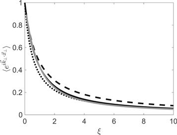
Figure 1. Characteristic function obtained for compound subdiffusion. Shown is the exact function as given by Equation (37) represented by the black solid line. Furthermore, we have shown the approximation of Equation (86) for  represented by the dotted line and
  represented by the dashed line. The gray solid line corresponds to the Karagiannidis & Lioumpas approximation as given by Equation (105).
Download figure:
Standard image High-resolution image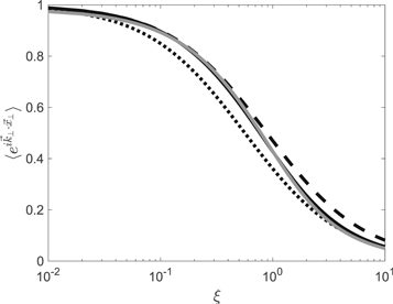
Figure 2. Same as Figure 1 but the results are shown as a semilogarithmic plot.
Download figure:
Standard image High-resolution imageThe particle distribution function in configuration space can be derived by combining Equations (85) and (21) to obtain
This last integral can be solved via (see, e.g., Gradshteyn & Ryzhik 2000)
where we have used the modified Bessel function of the second kind  . Thus, we finally find for the distribution function the following approximation
The latter function is visualized in Figure 3 where we can clearly see that the function is sharply peaked at the origin. We can explore the properties of this function at the origin by using (see, e.g., Abramowitz & Stegun 1974)

where we have used the Euler–Mascheroni constant γ. Clearly we find  . One can show by using the integral (see, e.g., Gradshteyn & Ryzhik 2000)

that the distribution function given by Equation (89) is correctly normalized. This can also be obtained simply by showing that approximation (85) satisfies condition (10). It is a strength of this approximation that normalization and initial conditions are satisfied exactly.
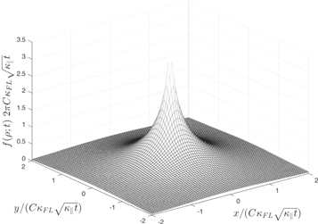
Figure 3. Distribution function  as given by Equation (89). This distribution is based on approximation (85).
Download figure:
Standard image High-resolution imageFurthermore, we can compute the distribution function projected on the x-axis. In order to do this we combine Equations (85) and (23) to obtain
The k⊥-integral can be evaluated by employing Cauchy's residue theorem. After some algebra we find
where we have used

Therewith we derive for the projected distribution function

The latter function is shown in Figure 4 for different times. Again the distribution is sharply peaked but now we find a finite result at the origin, namely
Below it will be shown that we find the exact second moment as given by Equation (61) if we set  . For this value we obtain
which is close to the exact result given by Equation (54).
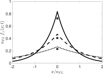
Figure 4. Projected distribution function as given by Equation (95) for different times  and
and  . This distribution is also based on approximation (85). Shown are the results for T = 0.1 (solid line), T = 1 (dashed line), and T = 10 (dotted line). Also shown is the exact value of the distribution at the origin (crosses). Those are given by Equation (54).
Download figure:
Standard image High-resolution imageWe can use Equation (95) to compute the nth moment via
where we assumed that n is even. For odd n the moments are, of course, zero due to symmetry. For the second moment we have n = 2 and Equation (98) becomes

and the running diffusion coefficient turns into

If we want to ensure that approximation (85) provides the correct second moment, we need to set  . The 4th moment can also easily be obtained from Equation (98) by setting n = 4 therein. We derive

With  this becomes

Since  this is very close to the exact result given by Equation (69). Problematic in Equation (98) is that the result sensitively depends on C. Therefore, for higher moments, the used approximation will be less accurate. Figure 5 shows a comparison of the moments up to n = 10 based on the exact formula given by Equation (70) and different approximations. Clearly we can observe a discrepancy for larger values of n.
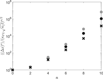
Figure 5. Exact moments as given by Equation (70) are represented by the black dots. All the odd moments are zero due to symmetry. Also shown are the moments based on Equation (98) for  . Those results are represented by the gray dots. The crosses represent Equation (117) which is based on the Karagiannidis & Lioumpas approximation.
Download figure:
Standard image High-resolution image4.2. The Karagiannidis & Lioumpas Approximation
In the current subsection we employ an alternative approximation. Karagiannidis & Lioumpas (2007) have stated that the complementary error function can be well approximated by

where A = 1.98 and B = 1.135. Therewith the function given by Equation (35) can be approximated by

and the characteristic function can be written as

Problematic here is that the initial condition (5) is not exactly satisfied. According to Equation (36) we have  for t = 0. In this case Equation (104) becomes

However,  which yields a condition very close to Equation (5). The same can be said about the normalization condition (10). Using Equation (104) in (21) yields
where we have used

and Equation (36). Employing approximation (104) in the fourth line of Equation (23), on the other hand, yields
Using (see, e.g., Gradshteyn & Ryzhik 2000)
the projected distribution function can be written as
We can compute the value of this distribution function at the origin. We can easily derive
which is similar but not identical compared to the exact value given by Equation (54) and the previous approximation given by Equation (97).
Calculation of the nth moment requires us to solve the integral

with the distribution function given by Equation (111). Therefore, in order to obtain the moments we need to evaluate the following two integrals (see, e.g., Gradshteyn & Ryzhik 2000)

and
where, of course, n is assumed to be an even integer number. Using these integrals in Equation (113) yields after some straightforward calculations
We can further simplify this by employing Equation (52). We derive
The moments obtained here are visualized in Figure 5. We observe that the moments computed based on the approximated distribution function (111) yields a result that is too small. Whereas the lower moments still agree well with the exact values, for higher moments there is clearly disagreement.
5. Results for Slab Turbulence and Comparison with Simulations
Usually it is assumed that subdiffusion occurs in the intermediate regime before normal diffusion is restored. The recovery of diffusion is related to the transverse complexity of the turbulence (see, e.g., Shalchi 2019 for a detailed discussion of the physics of perpendicular diffusion). However, if the latter effect is absent, compound subdiffusion is obtained as the final and stable result. Turbulence without transverse structure is also called slab turbulence. In this case the components of the spectral tensor are given by

All other components of this tensor are zero. For the spectrum  we use the Bieber et al. (1994) model

where we have used the normalization function

with the inertial range spectral index s. For the latter parameter we use  as motivated by the famous work of Kolmogorov (1941). The parameter
  is the bendover scale in the parallel direction separating the inertial range from the energy range. For the model spectrum of Equation (119) the field line diffusion coefficient becomes (see, e.g., Shalchi 2009)
This formula can be used to determine the field line diffusion coefficient which can then be combined with Equation (95) to obtain the particle distribution function in the perpendicular direction. This distribution function can now be compared to the simulations of Arendt & Shalchi (2018). In the latter article the following dimensionless quantities were used
where R is the dimensionless rigidity and  is the unperturbed gyro frequency with the electric charge of the particle q, the rest mass m, the speed of light c, and the Lorentz factor γ. The simulations are shown in Figures 6–8 for different parameter sets. In all those cases we set
  for the magnetic field ratio. Since the simulations were performed for different rigidities R, different parallel diffusion coefficients K∥ were obtained. The values for R and K∥ are given in the respective captions of Figures 6–8.
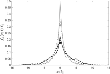
Figure 6. Distribution functions for pure slab turbulence and a magnetic rigidity of R = 0.1. Shown are the distribution functions for the different times T = 500 (gray lines) and T = 5000 (black lines). The solid lines are the simulations whereas the dotted lines represent the approximation obtained from Equation (95). The crosses are the values of the distribution function at the origin as obtained from Equation (54). The parallel diffusion coefficient is obtained from simulations and has the value  . The simulations are from Arendt & Shalchi (2018).
Download figure:
Standard image High-resolution image
Figure 7. Distribution functions for pure slab turbulence and a magnetic rigidity of R = 1. Shown are the distribution functions for the different times T = 500 (gray lines) and T = 5000 (black lines). The solid lines are the simulations whereas the dotted lines represent the approximation obtained from Equation (95). The crosses are the values of the distribution function at the origin as obtained from Equation (54). The parallel diffusion coefficient is obtained from simulations and has the value  .
.
Download figure:
Standard image High-resolution image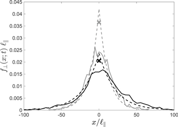
Figure 8. Distribution functions for pure slab turbulence and a magnetic rigidity of R = 10. Shown are the distribution functions for the different times T = 500 (gray lines) and T = 5000 (black lines). The solid lines are the simulations whereas the dotted lines represent the approximation obtained from Equation (95). The crosses are the values of the distribution function at the origin as obtained from Equation (54). The parallel diffusion coefficient is obtained from simulations and has the value  . The simulations are from Arendt & Shalchi (2018).
Download figure:
Standard image High-resolution image
As shown in Figures 6–8 we find indeed a sharply peaked distribution function. Problematic here is that in order to obtain a high resolution a huge amount of particles is required in the simulations. Close to the origin it is sometimes difficult to obtain the peak itself. However, apart from this problem, we find nice agreement between simulations and the results based on the Chapman–Kolmogorov approach.
Whereas using test-particle simulations to obtain distribution functions is a valid approach, it is also computationally expensive. An alternative is provided by using coupled stochastic differential equations as explained in Webb et al. (2006). One would expect that this approach might be more accurate than the simulations of Arendt & Shalchi (2018).
6. Summary and Conclusion
There are indications that perpendicular transport is subdiffusive after the ballistic regime. This subdiffusive behavior can be found until particles start to experience the transverse complexity of the turbulence. As soon as this happens, normal diffusion is restored. However, the subdiffusive behavior can persist for a long time in particular in turbulence with small Kubo numbers. Therefore, the theoretical exploration of particle distribution functions for the subdiffusive case is important.
The current work supplements the comprehensive work of Webb et al. (2006). We provided a very systematic calculation of all fundamental quantities based on Fourier transforms. This allows for an exact calculation of characteristic functions and moments. More problematic, however, is the analytical derivation of particle distributions in configuration space. In principle such distributions can be obtained but the results depend on complicated functions such as Meijer G-functions and generalized hypergeometric functions.
Due to the complications arising if particle distribution functions are calculated, we proposed two different approximations. In one case the distribution function can even be approximated by a simple exponential function. However, one has to be careful because for higher moments such approximations no longer provide a good approximation compared to the exact result (see Figure 5).
We have also compared our analytical findings with test-particle simulations (see Figures 6–8). For two of the considered parameter sets the simulations were performed in Arendt & Shalchi (2018) and for one set we performed the simulations anew by using the same test-particle code. Such a comparison is not without problems. The theory of compound subdiffusion predicts a sharply peaked function around the center of the distribution. In order to reproduce this peak via simulations, a very high number of particles is needed which makes such computations expensive. Despite these problems, we were still able to find agreement with analytical results and the simulations confirming our understanding of compound subdiffusion and the validity of the Chapman–Kolmogorov approach originally proposed by Webb et al. (2006).
Support by the Natural Sciences and Engineering Research Council (NSERC) of Canada is acknowledged.
Appendix A: Moments with Derivatives
The nth derivative of a Gaussian function can be written as (see, e.g., Abramowitz & Stegun 1974)

where we have used the Hermite polynomials  . Useful for later calculations is the relation

for even n and  for odd n. The numbers
  are also called the Hermite numbers. Here we have used

The Fourier transform of the perpendicular distribution function can be obtained from the first line of Equation (3). With the Fourier transform of the field line distribution function (25) this can be written as

Using

allows us to write

The nth moment, given by Equation (9), can then be written as
Using Equation (123) therein yields

Now we can substitute the function  therein by using the Gaussian function as given by Equation (30) to derive
With (see, e.g., Gradshteyn & Ryzhik 2000)

and Equation (124) we finally obtain

Using the relation (see, e.g., Abramowitz & Stegun 1974)

we find

As examples we can consider the cases n = 2 and n = 4. After employing  ,
,  , and
, and  we obtain
in agreement with Equations (61) and (69).
Alternatively we can employ Legendre's duplication formula (see, e.g., Abramowitz & Stegun 1974)

to derive
and
Using the latter two relations in Equation (135) yields

Employing Equation (52) allows us to write this as

in agreement with Equation (2.23) of Webb et al. (2006). Using Equation (52) two more times yields

As pointed out before, all these relations are valid only for even n.
Appendix B: Moments from Gaussian Distributions
An alternative for computing the moments was provided by Shalchi & Kourakis (2007) where one uses Equation (1) directly to find

where we have used the nth moment of the field line distribution  . For a Gaussian distribution of field lines this moment can be computed by employing Equation (24). We obtain
where n is again even. Using this and Equation (30) in Equation (143) yields
With Equation (132) we find

in agreement with Equation (135).
Appendix C: Transport Equation and Its Solution
In the main part of the text we derived the transport Equation (79) with the function  given by Equation (78). Combining the latter two equations yields
where  . In order to solve this equation we reverse the steps performed in the main part of the text. First we multiply our transport equation by
 ![$[\exp (-i{{\boldsymbol{k}}}_{\perp }\cdot {{\boldsymbol{x}}}_{\perp })]/{\left(2\pi \right)}^{2}$](https://content.cld.iop.org/journals/0004-637X/890/2/147/revision1/apjab6c69ieqn56.gif) and integrate over the whole two-dimensional space in order to derive
and integrate over the whole two-dimensional space in order to derive
Using integration by parts in the second and third lines yields
Using Equation (7) several times allows us to derive
where now  . This is in agreement with Equation (76). Via the relation (75) we can show that the solution is indeed

This is the solution for sharp initial conditions as given by Equations (5) and (6).