


Abstract
Gravity signatures observed by the Juno and Cassini missions that are associated with the strong zonal winds in Jupiter's and Saturn's outer envelopes suggest that these flows extend for several thousand kilometers into the interior. It has been noted that the winds seem to abate at a depth where electrical conductivity becomes significant, suggesting that electromagnetic effects play a key role for confining the winds to the outer weakly conducting region. Here, we explore the possible mechanisms for braking the zonal flow at depth in two model setups with depth-dependent conductivity and forced jet flow, i.e., in axisymmetric shell models and in more simple linearized box models that allow the exploration of a wide parameter range. Braking of the winds directly by Lorentz forces does not reduce their speed in the conducting region enough to be compatible with the inferred secular variation of Jupiter's field. Stable stratification above the depth where conductivity becomes significant can solve the problem. Electromagnetic forces drive a weak meridional circulation that perturbs the density distribution in the stable region such that the wind speed decreases strongly with depth, due to a thermal wind balance. For this mechanism to be effective, the stable layer must extend upward into a region of low conductivity. Applying the results of the linearized calculations to Jupiter suggests that the dissipation associated with the zonal winds can be limited to a fraction of the internal heat flow and that the jets may drop off over a depth range of 150–300 km.
Export citation and abstract BibTeX RIS
1. Introduction
The depth to which the strong alternating zonal winds at the surfaces of Jupiter and Saturn penetrate into the interior of the planets has been an open issue for decades. Some models assume that they are restricted to a thin atmospheric layer (Ingersoll & Cuzzi 1969), whereas others suggest that they extend deeply into the molecular hydrogen shell of the planets (Busse 1983). For Jupiter, an overview on observations and theoretical models is given in Vasavada & Showman (2005). Several attempts have been made to model jet formation in 3D numerical simulations of rotating and convecting spherical shells that represent the outer nonconducting envelope of gas planets, e.g., see Aurnou & Olson (2001), Christensen (2001, 2002), Heimpel et al. (2005, 2015), Kaspi et al. (2009), and Gastine et al. (2012). Those authors had some successes in producing multiple jets with strong zonal flow of approximately constant velocity on cylinders aligned with the spin axis, provided there is no frictional resistance on the lower boundary. However, with viscous friction at the bottom of nonmagnetic models, strong jet flow occurs only in equatorial regions outside the tangent cylinder, i.e., the cylinder coaxial to the rotation axis that touches the inner shell boundary at the equator (Jones & Kuzanyan 2009). The same holds for models that combine the generation of a strong dipole-dominated magnetic field in the deeper electrically conducting interior with flow in a poorly conducting outer envelope (Gastine et al. 2014; Jones 2014; Dietrich & Jones 2018; Duarte et al. 2018). Here, the location of the tangent cylinder that separates regions of strong and weak jet flow is given by the depth at the equator where conductivity becomes significant. The equatorial jet in the magnetic models, which stretches along cords that connect points on the outer boundary in one hemisphere to the mirror points in the other hemisphere, is confined by a combination of viscous and Lorentz forces. In nonmagnetic cases, the jets would extend much further toward the rotation axis (Duarte et al. 2013). Inside the tangent cylinder, boundary friction—or in the magnetic case, Maxwell stresses (Dietrich & Jones 2018)—effectively eliminate the jets.
The analysis of higher-degree gravity moments determined by the Juno and Cassini Grand Finale missions, respectively, strongly suggests that the jet flows extend to a depth of around 3000 km in Jupiter (Guillot et al. 2018; Iess et al. 2018; Kaspi et al. 2018) and around 8000 km in Saturn (Galanti et al. 2019; Iess et al. 2019). The nonuniqueness of gravity inversions precludes a determination of how precisely the wind velocity changes with depth (Kaspi et al. 2018). In principle, a deep circulation that is unrelated to the surface winds could also explain the observed gravity signal (Kong et al. 2018). Furthermore, some technical issues of how to link the gravity signal to the flow dynamics remain (Zhang et al. 2015; Galanti et al. 2017; Wicht et al. 2020). Nevertheless, the zonal wind effect on the odd-degree gravity moments of Jupiter, which is not masked by the rotational deformation of the planet (Kaspi 2013), along with the finding that a good match to these moments can be found based on a simple downward extension of the surface winds (Kaspi et al. 2018), strongly indicates that their speed must be significant to more than 1000 km depth. Moore et al. (2019) find that the secular variation of Jupiter's magnetic field is consistent with advection of field lines by the zonal winds at a depth of (0.93–0.95)rJ, where electrical conductivity becomes significant (rJ is Jupiter's mean radius). The data require that the wind velocity has dropped to several cm s−1 at that depth, down from the several tens of m s−1 at the surface.
The forcing of the zonal flow could either be associated with shallow moist convection in a weather layer or with deep convection in the molecular hydrogen envelope. In either case, energy is pumped in an inverse cascade from turbulent small-scale motions into large-scale jets (Vasavada & Showman 2005). In a rotationally dominated regime, correlations of the different components of the small-scale flow lead to Reynolds stresses that cause a latitudinal transport of angular momentum. Cloud tracking at Jupiter (Salyk et al. 2006) and Saturn (Del Genio et al. 2007) has revealed a momentum flux from small eddies into the zonal jets. The number of jets and their direction—prograde near the equator on Jupiter and Saturn, and retrograde at Uranus and Neptune—could be affected by the proportion between internal and external heat flow (Liu & Schneider 2010) or the abundance of water (Lian & Showman 2010) in the different planets. It has been pointed out by Showman et al. (2006) that irrespective of whether the forcing is shallow or deep, due to the Proudman–Taylor theorem that holds in a nearly inviscid rotating system at low Rossby number, the jets themselves could penetrate deeply into the fluid. Detailing how the jets are forced is not in the focus of the present study. Rather, we address the physical mechanism that can limit the penetration depth.
The electrical conductivity increases gradually with depth in the gas planets, from virtually negligible values in the top few thousand kilometers, through a semiconducting region with steeply increasing values due to hydrogen ionization, to metallic conductivity at greater depth (French et al. 2012). It has been noted that the depths where the winds abate according to the gravity analyses coincide with the levels where electrical conductivity becomes significant (Kaspi et al. 2018; Galanti et al. 2019). This may suggest that Lorentz forces due to the electrical currents induced by the interaction of the jet flow with the intrinsic magnetic field of the planet brake the zonal flow. Liu et al. (2008) argued that the requirement to limit the ohmic dissipation associated with the induced currents to plausible values sets a limit on the depth (or conductivity value) of wind penetration that is in rough agreement with the gravitationally inferred penetration depth. They also showed that, at this depth, the Lorentz forces would be far too small to directly break the Proudman–Taylor theorem. The constraint on ohmic dissipation is not compelling, as argued by Glatzmaier (2008) and Wicht et al. (2019a), because Liu et al. (2008) derived it under the assumption that the magnetic field is essentially unmodified by the zonal winds. This does not hold when the winds penetrate beyond the depth where the local magnetic Reynolds number exceeds one. Nonetheless, there can be little doubt that, at a depth where the conductivity is high, the velocity should have dropped to the range of cm s−1 that is expected for Jupiter's dynamo region (Christensen & Aubert 2006), in agreement with the estimate from the secular variation of Jupiter's field (Moore et al. 2019). Wicht et al. (2019b) predict the pattern and amplitude of the magnetic field produced by the winds, and Duer et al. (2019) present a method for the joint analysis of gravity and magnetic secular variation data, which will allow to better constrain the depth of the winds. These magnetic signatures may be revealed by the ongoing measurements of the Juno mission.
Stably stratified layers may exist inside the gas planets that can have an effect on the variation of the zonal winds with depth. Guillot & Gautier (1994) suggested that a zone of radiative heat transfer exists at temperatures in the range of 1200–2000 K, corresponding to a radius range of (0.97–0.99)rJ in Jupiter. However, if significant amounts of alkali metals are present, the opacity would be high enough to eliminate the radiative zone (Guillot et al. 2004). Segregation of helium due to its limited miscibility with hydrogen is a likely candidate for creating a stable layer with a gradient in He concentration, especially in Saturn (Schöttler & Redmer 2018). However, the reduced miscibility is associated with the metallization of hydrogen, and the stability region that is formed by this mechanism is probably too deep for affecting zonal flows. Debras & Chabrier (2019) studied models of Jupiter's internal structure in the light of the precise measurements of higher even-degree gravity coefficients by the Juno mission. They concluded that, in order to satisfy these and the atmospheric heavy element abundance determined by the Galileo mission, a region of compositional (and entropy) change must exist between inner and outer convecting regions. In their models, the compositionally stratified region could be located between (0.8-0.9)rJ and 0.95rJ.
Using simple circulation models, Showman et al. (2006) considered the interaction of zonal flow, forced in a thin layer at the very top, with a stably stratified region. They showed that a meridional circulation is set up and perturbs the thermal (or buoyancy) structure in the stable region such that the zonal flow velocity decreases with depth due to a thermal wind balance. In a steady state, the meridional circulation is controlled by a balance between driving forces and frictional or dissipative effects, which are parameterized in their model. In the case of negligible friction, the winds extend unabated through the stable region. In simplified convection models in a rotating annulus, Jones et al. (2003) found that boundary friction, while diminishing the amplitude of zonal flows, may be important for obtaining multiple jets inside the tangent cylinder. Liu et al. (2013, 2014) considered fully convecting outer envelopes of Jupiter and Saturn, but assume that the wind speed decreases with depth due to a thermal wind balance. They suppose that the energy transferred at shallow depth into the zonal winds is lost by ohmic dissipation in the (semi-)conducting region. They argue that convection homogenizes entropy along the spin axis, but allows for entropy gradients perpendicular to the spin axis, which are then the cause for the thermal wind effects. While they construct models with an entropy structure that ensures a drop-off of the zonal flow that is sufficiently strong to limit the ohmic dissipation to a reasonable amount, the physical mechanism that produces such an entropy structure, well-correlated with the jets, remains an open question. Three-dimensional convection simulations that exhibit zonal jets do not show the required entropy distribution.
The present study revisits the physical mechanism for the variation with depth of zonal winds in a rotating magnetized planet with radially varying electrical conductivity. We use simplified axisymmetric models of zonal flows driven by an ad hoc volume force, which is assumed to represent the action of Reynolds stresses created by turbulent convection. These models are necessarily far from planetary values, with regard to some essential control parameters, and are not meant to quantitatively predict the wind structure inside Jupiter or Saturn. Rather, they serve to illuminate some of the principles that govern the dynamics of such a system. In addition, two-dimensional and linearized models in Cartesian geometry are used to extend the parameter range all the way toward plausible planetary values. They allow quantitative inferences regarding the structure of deep-reaching zonal winds and the conditions for their compatibility with all known constraints.
2. Model Setup and Governing Equations
We consider axisymmetric spherical shell and 2D Cartesian models of flow that is driven by an imposed volume force and is subject to strong rotational effects. The background stratification of the fluid is stable below a certain depth and is neutral above. The electrical conductivity varies strongly with radius (height). In an imposed magnetic field, currents are induced and the associated Lorentz forces affect the circulation. The spherical shell models serve to illustrate the physical effects and to show that the simplifications in the Cartesian models, which reach much more extreme parameter values, do not qualitatively change the results. The spherical shell simulations are done with the Boussinesq approximation (constant background density). Gastine & Wicht (2012) found, in anelastic convection simulations, that the properties of the jets did not differ significantly from those in Boussinesq models. The Cartesian models in the present work employ variable background density in the anelastic approximation.
We solve for velocity  , magnetic field
  , and codensity perturbation c from a reference state Co. Codensity combines the effects of entropy perturbations and deviations of composition from a background state (Braginsky & Roberts 1995). It is defined as
  , where T' and χ' are deviations in temperature and composition, respectively, from an adiabatic and well-mixed reference state, α and β are expansion coefficients, and
  is the unperturbed reference density. We employ nondimensional variables where the basic length scale is the shell thickness or layer depth D, and time is scaled by D2/κo. Magnetic field is scaled by
  and codensity by
  , where
  is the codensity gradient dCo/dr at the lower boundary, κo is a reference diffusivity for codensity, ρo is the reference density at the bottom of the system, μo the vacuum permeability, ηo the magnetic diffusivity at the bottom, and Ω the rotation rate. In their general form, the governing equations are


The unit vector  indicates the direction of the rotation axis, and
  the radial direction (in the Cartesian models, both directions coincide). Here, Π is an effective pressure (Braginsky & Roberts 1995);
  is the viscous force term, equal to
  in the Boussinesq case and more complex in the anelastic case (e.g., Gastine & Wicht 2012); and
  is the imposed driving force per unit mass (scaled with
  ).
).
The four nondimensional control parameters are an Ekman number based on the codensity diffusivity

a Rayleigh number describing the degree of stratification in the stable layer

the Prandtl number

and the Roberts number

The Roberts number is related to the more common magnetic Prandtl number Pm = ν/ηo by q = Pm/Pr. Gravity g is assumed to be constant, whereas the codensity diffusivity κ and magnetic diffusivity η are depth-dependent. In the case of κ, the diffusivity is assumed to represent an effective value, enhanced by turbulent mixing, which is smaller in the stably stratified region than in the overlying freely convecting region. The degree of stability in the stratified region is expressed by the nondimensional Brunt–Väisälä frequency

whose dimensional value is  , with ρ' being the deviation of density from that of the isentropic and compositionally homogeneous reference state. For Jupiter, with a nonadiabatic density increase of 0.5–2.5% distributed over 2500–7500 km as in the models by Debras & Chabrier (2019),
  would be approximately in the range 0.8–3.
2.1. Setup of Spherical Shell Models
We solve the above equations in a spherical shell with inner radius ri = 4 and outer radius ro = 5 in the Boussinesq limit, i.e.,  = 1. Spherical coordinates (r, θ, ϕ) are used and only axisymmetric flow is considered, i.e., ∂/∂ϕ = 0. The dimensionless background codensity gradient
  equals one at ri and decreases mildly with r so that the total flux
  remains constant up to r − ri < 0.32. For r − ri > 0.48, it is zero with a smooth transition in between. The diffusivity κ is set to the reference value κo in the upper part of the shell (i.e., nondimensional value is one), and is reduced tenfold in the stable lower region, also with a smooth transition. The driving force is specified as
  , where Af is the amplitude of forcing,
  is the unit vector in azimuthal direction, s = r sin(θ) is the distance to the rotation axis (or cylindrical radius). The forcing is restricted to radii larger than rf, which is set here to 4.7, i.e., forcing is limited to the top 30% of the shell. Setting
  , the radial dependence is, for r > rf:

Figure 1(a) shows the radial variation of the background codensity, of the codensity diffusivity, and of the forcing function. Seven bands of alternating zonal flow inside the tangent cylinder  are driven in each hemisphere by specifying an s-dependence of the forcing as

Friction outside the tangent cylinder is less than it is inside. To avoid excessive differences in zonal flow velocities between the two regions, the forcing function is attenuated in the s-direction, setting h(s) to one for s < 3, to  for 3 < s < 4, and to
  for s > 4. The complete pattern of the forcing function is displayed in Figure 2(b).

Figure 1. (a) Radial variation of background codensity Co (black), forcing function f (red), and diffusivity κ (blue) used in the spherical models. (b) Radial variation of magnetic diffusivity η used in the spherical models (black). The profile shown by the blue line is used in the Cartesian models where the vertical coordinate z replaces r − ri.
Download figure:
Standard image High-resolution image
Figure 2. Axisymmetric models of forced zonal flow, uϕ, depicted by color in panels (a), (c), (e), and (g), where contour lines show the meridional flow. (a) Nonmagnetic case 1 without stable layer; (b) pattern of driving force used in all cases; (c)–(d) nonmagnetic case 2 with stable layer, where panel (d) shows codensity perturbation; (e)–(f) magnetic case 4 with Bo = 5 without a stable layer, where panel (f) shows Bϕ in color and poloidal field lines; (g)–(h) magnetic case 5 with Bo = 1 and a stable layer, where panel (h) shows codensity perturbation and poloidal field lines. Contour steps for uϕ are shown by color bars (oversaturated in the equatorial region in panel (e)), those for Bϕ are 0.0001 in (f), and those for codensity perturbation in (d) and (h) are 0.0008. The vertical line in (e) indicates the position of the cord at s = 3 for which profiles are shown in Figures 3 and 4. Values on this cord are listed in Table 1 for all models.
Download figure:
Standard image High-resolution imageThe boundary conditions are impermeable and shear-stress free at ro and at ri. We note that the forcing function implies a net torque on the shell; in the absence of magnetic coupling to the interior, which is immobile in the rotating reference frame, this would imply a continuous spin-up. That is taken care of by simply removing the solid-body rotation part from the solution. The condition for the codensity perturbation is c = 0 at ro and dc/dr = 0 ar ri. The magnetic field at ro is matched with a potential field above the shell. An axial dipole field with amplitude Bo at the poles is imposed as a boundary condition at ri. All other magnetic field components are matched with a field that is obtained by solving Equation (2) with  and η = 1 in the region inside the sphere. This means that the electrical currents associated with a toroidal magnetic field, which is induced by the flow in the shell, can close through the highly conducting interior. The discontinuity in horizontal velocity at ri between the flow in the shell and the immobile core implies a complex nonlinear jump condition for the radial derivative of the toroidal field at the interface; see Equations (5.8)–(5.10) in Kuang & Bloxham (1999).
To solve the equations numerically, a pseudo-spectral dynamo code that expands all variables in spherical harmonic functions in the angular variables and in Chebychev polynomials in radial direction is used (Christensen & Wicht 2015). Here, it is stripped down to only axisymmetric modes. We use 341 Legendre polynomials in the θ-direction and 97 Chebychev polynomials in the radial direction. By using a grid-stretching technique, we condense the radial grid points in the transition region between the stable and the unstable parts. The system is marched in time until a stationary solution is reached.
In all models presented here, the Ekman number has been set to Eκ = 10−5, and the Prandtl number Pr and the Roberts number (at the bottom) q are one. The magnetic diffusivity increases exponentially

where the change from the inner boundary to the outer boundary is by a factor  . The setup and the choice of parameters was not made with the aim to represent conditions for Jupiter or Saturn as closely as possible. Instead, the models are meant to explore and illustrate general principles that govern the depth-dependence of zonal flow.
3. Results for Spherical Shell Models
We discuss a sequence of models with increasing complexity to highlight the effects of a stable layer and of a magnetic field on the zonal flow, first separately and then in combination. The amplitude of forcing has been set to an arbitrary value of Af = 2500 in most simulations, which is small enough to render the nonlinear terms in the equations almost negligible. The question of their relevance is addressed by running a case with much stronger forcing. Model parameters and some results are summarized in Table 1.
Table 1. Axisymmetric Spherical Models
| Case |

|
Bo | Af |

|

|

|
r50 − ri | r10 − ri | Dohm | Ru |
|---|---|---|---|---|---|---|---|---|---|---|
| 1 | 0 | 0 | 2500 | 16.0 | 0.056 | ⋯ | ⋯ | ⋯ | 0% | 0.935 |
| 2 | 4.24 | 0 | 2500 | 22.8 | 0.019 | ⋯ | 0.213 | 0.048 | 0% | 0.517 |
| 3 | 0 | 1 | 2500 | 0.163 | 0.041 | 0.0045 | ⋯ | ⋯ | 41% | 1.080 |
| 4 | 0 | 5 | 2500 | 0.036 | 0.016 | 0.0008 | 0.111 | 0.048 | 56% | 0.120 |
| 5 | 4.24 | 1 | 2500 | 17.8 | 0.013 | 0.0016 | 0.353 | 0.238 | 18% | 0.0013 |
| 6 | 4.24 | 1 | 250000 | 1769 | 1.241 | 0.162 | 0.352 | 0.236 | 17% | 0.0013 |
Note. Maximum values of  , uθ and Bϕ are taken at s = 3. Here, r50 and r10 are the radii at which the zonal flow velocity has dropped to 50% and 10%, respectively, of its surface value. We define Dohm as the fraction of dissipation by ohmic losses, and Ru is the ratio of rms velocity at the bottom to that at the surface inside the tangent cylinder.
Download table as: ASCIITypeset image
Before discussing the results, we consider two equations that hold in a steady state when nonlinear terms can be neglected, and which are useful for interpreting the results. With these approximation, the ϕ component of Equation (1) is, in the Boussinesq case:
where the current density is  and
and  is the current-free imposed dipolar field. Here, s is the cylindrically radial coordinate perpendicular to the rotation axis. The viscous force term in ϕ-direction is
  . The equation tells that the meridional circulation is controlled by the forcing term FD, by viscous friction (insignificant in a real planet), and by the Lorentz force associated with an induced current. The ϕ component of the curl of Equation (1) results in
This is, aside from the viscous term where  is vorticity, a thermal-magnetic wind equation that relates the change of the jet velocity along the direction of rotation to the codensity perturbations and magnetic forces, and is therefore key to our study.
3.1. Nonmagnetic without Stable Stratification
Figure 2(a) shows the velocity field in the nonmagnetic case without a stable layer. The zonal flow satisfies the Proudman–Taylor theorem almost perfectly, i.e., it hardly varies with z. The meridional circulation is weaker than the zonal flow. In the top region, the force driving the zonal flow is balanced by the Coriolis force associated with the meridional circulation according to Equation (13), hence it implies a flow in the s-direction. At depth, the direction of us must reverse because of mass conservation, and here the Coriolis force must be balanced by viscous friction in the bulk of the fluid, resulting in a distributed return flow, when Lorentz forces are unavailable.
3.2. Nonmagnetic with Stable Stratification
We next consider nonmagnetic case 2 with a strongly stable layer ( ) in the lower part of the shell. Inside the tangent cylinder, the jet flow in the neutrally stable region is slightly stronger than in the absence of a stable region (Figure 2(c)). In the stable layer, it decreases with depth in amplitude, although it remains significant down to the lower boundary. The meridional circulation grazes the top of the stable region where it creates a codensity anomaly by lateral advection, which is strongest in the upper part of the stable layer (Figure 2(d)). The zonal flow velocity decreases with depth, due to the associated thermal wind effect given by the first term on the rhs of Equation (14). The jets become slanted, i.e., they extend in the radial direction in the stable layer rather than along the z-axis. The ratio of the rms velocity on the bottom boundary to that at the surface inside the tangent cylinder (s < 3.95) is listed in Table 1 under the entry Ru. In the cases with a stable layer but without magnetic field, Ru is still approximately 0.5 at
  . This simulation suggests that, in a real planet, a stable layer alone—without some additional resistive effect on the flow—may be rather inefficient in reducing zonal flow velocities with depth.
3.3. Magnetic without Stable Stratification
We now turn to cases 3 and 4, which lack a stable layer but have an exponentially varying electrical conductivity and an imposed dipolar field. While the jet outside the tangent cylinder remains strong, the amplitude of the zonal flow inside the tangent cylinder is reduced by more than two orders of magnitude compared to cases 1 and 2 (Table 1 and Figure 2(e); note the difference in color scale between different velocity plots in Figure 2). To obtain the same jet velocity as in the nonmagnetic cases, much stronger forcing would be required. By implication, the amount of energy dissipation would be much higher. With a magnetic field amplitude Bo = 1 (case 3), which is equivalent to an Elsasser number Λ = 1 being reached for the conductivity at the bottom boundary, the jet velocity hardly changes with depth all the way down to the lower boundary. The Elsasser number is a measure for the ratio between Lorentz forces and Coriolis forces, and is defined as
When the magnetic field strength is increased to Bo = 5 (case 4), with Λ = 25 being reached at the bottom, the surface wind speed inside the tangent cylinder drops by another factor of four compared to the case with Bo = 1. In contrast to the case with the weaker field, with Bo = 5 the wind velocity changes with depth in the lowermost part of the shell and drops by an order of magnitude toward the bottom (Figure 3). The same effect would be achieved for Bo = 1 by increasing the conductivity by a factor of 25. Note that values of Λ > 1 are not reached in the semiconducting regions in the gas planets, but require fully metallic conductivity. The zonal flow induces a magnetic field in the ϕ-direction (toroidal field, Figure 2(f)) in the lowermost part of the shell. However, the currents associated with this field, which run in the (s, z) plane, are not directly related to the decrease of the zonal velocity, which requires a jϕ current (Equation (14)). Instead, the Lorentz force associated with the toroidal field currents balances the Coriolis force of the meridional circulation in this depth range according to Equation (13). Figure 3 shows for the center of one of the jets inside the tangent cylinder, at s = 3, the variation of the zonal velocity and of the s component of the velocity as function of the z coordinate. Also shown is the driving force FD and the ϕ component of the Lorentz force, taken from the simulation. Both forces are multiplied by 2/Eκ in the plot. They fall almost exactly on the curve for us, showing that the viscous term in Equation (13) is insignificant in this simulation. Compared to the previously discussed cases, where viscous forces balanced the meridional return flow, this role is now taken by magnetic forces. Finally, the interaction of the meridional flow with the magnetic field then gives rise to an electrical current jϕ, which relates to the drop of the zonal flow velocity with depth according to Equation (14). We also note that the Elsasser number, which varies strongly in the shell (mainly because of the variable conductivity), has a value around one at the point of the strongest decrease of uϕ(z).

Figure 3. Velocity and forces along a cord at s = 3 (shown as black line in Figure 2(e)) for case 4 with a strong magnetic field and no stable layer. Here, zo is the value of z at the inner boundary and FL is the ϕ component of the Lorentz force. Forces have been multiplied by 2/Eκ.
Download figure:
Standard image High-resolution imageTo achieve the same zonal flow velocity inside the tangent cylinder as in the nonconducting cases 1 and 2, the driving force—and hence, the power input and the dissipation—had to be increased by factors of approximately 100 for Bo = 1 and 500 for Bo = 5. At least in the quasi-linear regime of these simulations, where the imposed background field is not significantly altered, strong zonal flows do not abate drastically before they reach a depth of high conductivity. This seems incompatible with the secular variation and possibly the magnetic field geometry of Jupiter. An additional mechanism is needed to reduce the wind speed with depth.
3.4. Magnetic with Stable Stratification
While the simulations discussed so far confirm and illustrate some principles that had been conjectured before and studied in other models (e.g., Showman et al. 2006; Liu et al. 2008), we now enter new terrain by combining a stable layer with magnetic effects. Case 5, where Bo = 1, is shown in Figures 2(g)–(h). The zonal flow inside the tangent cylinder has a slightly larger surface velocity than in the nonmagnetic case without stable layer. In contrast to that case, the zonal flow velocity in case 5 starts to drop at mid-depth and decreases most sharply in the upper part of the stable layer (Figure 4(a)). Its value close to the inner boundary is approximately 1/1000th of the surface velocity. This drop-off is exclusively related to a thermal wind effect, as shown in Figure 4(b), which compares  with the prediction from a thermal wind balance, i.e., with RaPrEκ/(2r) ∂c/∂θ at s = 3. The two lines plot almost exactly on each other, showing that neither the Lorentz force term in Equation (14), which is essential in case 4 without stable layer, nor the viscous term play a role. However, the Lorentz force is important for the meridional circulation, which causes the codensity perturbation that is essential for the drop-off with depth of the jet velocity. In Figure 4(c), we compare the velocity in the s-direction on the cord with s = 3 with the various force terms in Equation (13). The Lorentz force is not the only contributor at the depths where the driving force FD has dropped to zero, but is essential to balance FD in the meridional flow equation. Without it, in case 2, where viscosity is the only antagonist to the driving force, the meridional circulation is unable to penetrate deeply into the stable layer and to create a codensity anomaly that kills the jets before they can reach the bottom boundary. However, in the magnetic case with a stable layer, the viscous force in Equation (13) is of the same magnitude as the Lorentz force. This contrasts with the strongly magnetic but neutrally stratified case 4, where the viscous contribution is insignificant. This difference is not surprising, as uϕ is almost three orders of magnitude smaller in the neutrally stratified case. That viscous effects are rather large is also shown by the fact that dissipation by ohmic losses is generally smaller than viscous dissipation, especially also in case 5 (Dohm in Table 1). In a real planet, the opposite might be expected.

Figure 4. Plots along the cord at s = 3 for magnetic case 5 with a stable layer, similar to Figure 3. The stratification is neutral above the upper horizontal line and assumes its full value of  = 4.24 below the lower line. (a) Zonal flow and toroidal field. Here, Bϕ is multiplied by 104. (b) Comparison of terms in the vorticity Equation (14). Here, FB is the buoyancy (or thermal wind) term, multiplied by
  . The magnetic and viscous terms in Equation (14) make no significant contribution. (c) Comparison of terms in the ϕ component of the equation of motion Equation (13). Forces are multiplied by Eκ/2, FL is the Lorentz force term.
Download figure:
Standard image High-resolution imageAll cases discussed so far have been calculated in an almost linear regime. The Rossby number  , which describes the ratio between the nonlinear inertial term and the Coriolis term, reaches only up to 2 × 10⁻⁴. In the magnetic cases, the amplitude of the induced field is much smaller than that of the imposed field, and the Lorentz force arising from the interaction of the induced currents with the induced field can be ignored. The Rossby number for Jupiter's zonal jets at higher latitudes is (1–2) × 10−2. This Rossby number is reached in case 6, where the forcing amplitude Af has been increased by a factor of 100 compared to that in case 5. Here, the amplitude of the induced toroidal field reaches 17% of that of the imposed dipole field. Nonetheless, all properties of the solution still scale almost linearly compared to case 5, i.e., they are larger by a factor of 100 (Table 1). The depth and the shape of the drop-off of the jet flow are essentially the same as in case 5. This suggests that linearized models, such as those studied in Section 4, can be meaningful for the gas planets.
To summarize the results of this section, only the combination of a stably stratified layer with electromagnetic effects seems to be able to simultaneously meet two requirements: (1) for a given moderate forcing, strong zonal jets develop at the surface; and (2) at the same time, their velocity drops off to very small values before the jet has reached a depth with high electrical conductivity. While the axisymmetric models are useful to illustrate the main physical effects, their excessive viscosity prevents them from being used directly for a quantitative comparison with the gas planets. This would require much lower values of the Ekman number that cannot be reached, for technical reasons, in such simulations.
4. Linearized Cartesian Models
Simulations in Cartesian geometry are numerically cheaper than spherical shell calculations. In addition, the similarity of the weakly forced and the strongly forced spherical solutions suggests that nonlinear effects are secondary, at least in the magnetic case with a stable layer. We therefore employ linearized Cartesian calculations that reach the relevant planetary parameter regime. This enables us to make (semi-)quantitative predictions for gas planets.
4.1. Model Setup and Equations
The model setup is illustrated in Figure 5. A layer of unit depth (0 < z < 1) is assumed. Gravity and rotation are aligned and parallel to the z-axis. The imposed magnetic field  is constant and points in the z-direction. This would approximately represent the situation close to the poles in a spherical shell. The results of the axisymmetric shell models suggest that the behavior is not fundamentally different at lower latitudes inside the tangent cylinder. Cartesian models with the magnetic field pointing in the x-direction (not discussed in detail here) show similar results. The system is periodic in the x-direction, which replaces latitude or the s-coordinate in a sphere. A flow in the y-direction (which replaces longitude) is driven by an imposed sinusoidal force FD = Af f(z) sin(kx). The system is two-dimensional, i.e., ∂/∂y = 0. Here, f(z) has the same form as in Equation (10), with z replacing r. Forcing is nonzero in the range 0.7 < z < 1.0.

Figure 5. Schematic drawing of the Cartesian model.
Download figure:
Standard image High-resolution imageEquations (1)–(4) are written in terms of the following dependent variables: U = uy for the jet flow, the stream function ψ for the meridional flow that is obtained as  , c for codensity perturbation, bz for the perturbation of the z-component of the poloidal field, and jz for the z-component of the current density that is associated with the toroidal field. In contrast to the Boussinesq spherical shell models, we use here the anelastic approximation. For simplicity, we assume an exponential density variation with a constant scale height dρ.
The equations are linearized, assuming for the perturbation field  and for the meridional flow


The viscous term in Equation (17) is
The components bx, by that appear in these equations are obtained from the primary variables bz, jz by using  ,
,  , and
, and  .
.
The variables are expanded in sine or cosine functions in the x-direction, e.g.,  . Because of the linearization, all wavenumbers k decouple. Equations (16)–(20) reduce to a set of five coupled ordinary differential equations in z. The same boundary conditions as in the spherical models are assumed, except for the magnetic field on the lower boundary, which is matched with a field that is obtained for an exponentially decreasing diffusivity η in the substratum z < 0. This condition can be implemented analytically for a given horizontal wavenumber k. The background codensity gradient changes around z = zs from stable (
 ) in the lower part to neutral above. The transition is smoothed again, but the transition interval is narrower than in the spherical shell simulations and restricted to zs ± 0.01. The reference value for codensity diffusivity κo is now that in the lower layer. We assume that, in the upper region, the effective diffusivity by turbulent convection is so efficient that it practically wipes out any significant codensity differences. This means codensity is not solved for in that region, and the condition c = 0 is applied at the upper end of the stable region at z = zs + 0.01.
We note that, in the case of stationary solutions (∂/∂t = 0), which are the only ones considered here, the Roberts number q can be eliminated from the equations by introducing a modified variable for the magnetic field perturbation and the current density,  and
and  . For the simulations, where we set q = 1, this is not important. However, it becomes relevant when we scale the model results to real planets.
Equations (16)–(20) are solved for a specific wavenumber k, where derivatives ∂/∂x turn into factors ik, by a finite-difference scheme, using up to 4000 equidistant points in z. The equations are marched in time using an implicit scheme until a steady state has been reached. The solutions are linear in Af, and therefore the forcing amplitude can be easily adjusted such that all reported solutions have a velocity of U = 1.0 at z = 1. We report results for Eκ in the range between 10−8 and 10−11, and Rayleigh numbers Ra between 1016 and 3 × 1024. In the cases with the highest values of the Rayleigh number, i.e., Ra ≥ 1024 for zs = 0.7 and Ra ≥ 1021 at zs = 0.6, the numerical scheme becomes unstable for our standard setup. A stable solution can be obtained by applying the boundary conditions for U, ψ, and c not at z = 0 but at z = 0.35, and by setting these variables to zero below that depth. This is justified because at the highest values of Ra, all three variables assume almost zero values in the lower part of the domain. Comparison to a case in which a converged solution could also be obtained for the standard setup showed only very slight differences.
4.2. Choice of Parameters
We strive at using parameters that are close to conditions in Jupiter as far as possible. We assume that the model domain covers the outer 10% of Jupiter, i.e., z = 0 corresponds to 0.9rJ. We use a superexponential variation of electrical conductivity. Figure 6 shows the conductivity values in the upper 12% of Jupiter's interior according to quantum mechanical ab initio simulations by French et al. (2012). They are decently fitted by
Identifying a radius of 0.9rJ with the lower boundary of the Cartesian model, Equation (22) translates into a nondimensional magnetic diffusivity of
which is shown by the blue line in Figure 1(b) and is applied in the Cartesian models. To avoid numerical problems, the values are capped at a diffusivity  . Equation (22) gives a conductivity of 6.9 × 10⁴ S m−1 at 0.9rJ. Together with a density at this depth of 577 kg m−3 (Nettelmann et al. 2012) and Ω = 1.76 × 10⁻⁴ s−1, this results in a magnetic field scale of 1.2 mT. Jupiter's dipole field has, on average, a strength of 0.6 mT in the region (0.9–1.0)rJ. Hence, a nondimensional value of Bo = 0.5 is appropriate and is applied here.

Figure 6. Conductivity in the upper part of Jupiter's interior, according to French et al. (2012) (circles) and fit by Equation (22).
Download figure:
Standard image High-resolution imageThe average distance between a prograde jet and its retrograde neighbors at the surface of Jupiter is approximately 4° or 4800 km. With the depth of the simulation box corresponding to 0.1rJ or 7000 km, the nondimensional wavenumber is around  , and we fix this value in our calculations.
We set the nondimensional density  equal to one at z = 0. The scale height is quite variable in the molecular hydrogen envelope of the gas planets. For our calculations, where a constant scale height is assumed, we pick a nondimensional value of dρ = 0.43429, corresponding to a density ratio Δρ from top of bottom of ten. This roughly matches the scale height in Jupiter at about (0.95–0.96)rJ, or z = 0.5–0.6 in the simulations box, which is not far from where the drop-off of the jet flow occurs in our models.
We compare results for two locations of the upper boundary of the stable layer, zs = 0.6 and zs = 0.7, corresponding to 0.96rJ and 0.97rJ, respectively. As we will see, a stable region that extends rather high up turns out to be essential for meeting constraints on the power that is driving zonal winds in Jupiter. We calculated a series of models for each value of zs by varying the Rayleigh number over a wide range, and choosing the Ekman number Eκ such that the fraction of viscous dissipation of the total (viscous plus ohmic) dissipation is always below 5%. At higher Rayleigh number, this requires lower values of the Ekman number.
4.3. General Properties of the Solution
Figure 7 shows depth profiles for a case with zs = 0.7 at a high value of the Rayleigh number and low Ekman number. The jet velocity (full line in Figure 7(a)) stays constant above the stable region and drops sharply at the very top of the stable layer to very small values. The meridional circulation (ux, uz) is approximately seven orders of magnitude weaker than the jet flow. It vanishes at depths not far below the top of the stable layer. As was already seen in the spherical shell simulations, the decrease of U = uy is associated with the thermal wind term FB (the last term in Equation (17)), whereas the magnetic term FL does not contribute (Figure 7(b)). The codensity perturbation causing the thermal wind effect is created by the meridional flow, which results from the Lorentz force associated with the induced electrical current component jx as the only significant antagonist to the driving force FD (Figure 7(c)). This contrasts with the spherical shell model, where viscous friction still played a significant role in the meridional force balance (compare Figure 4(c)).
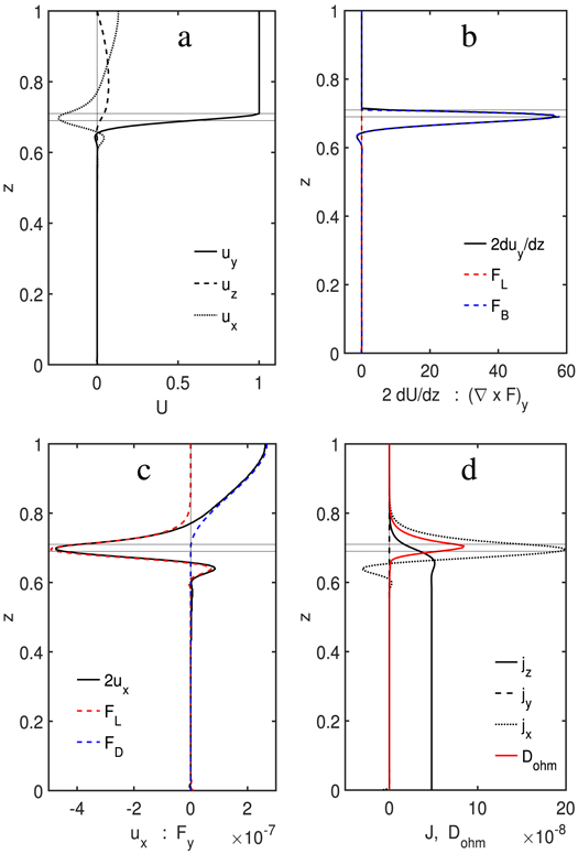
Figure 7. Depth-dependent profiles for a Cartesian case with Ra = 3 × 10²³, Eκ = 10−11 and zs = 0.7. Horizontal lines indicate the boundary of the stable layer. (a) Velocity components; ux and uz are multiplied by 106. (b) Depth variation of the jet velocity compared with the thermal wind term FB and magnetic wind term FL in Equation (17). (c) Meridional flow component ux (black line) compared with the driving force FD and the y-component of the Lorentz force in Equation (16). (d) Current density and ohmic dissipation. Force terms in (b) and (c) are multiplied by Eκ.
Download figure:
Standard image High-resolution imageThe electrical current (jx, jz) associated with the toroidal magnetic field is induced by the interaction of the zonal flow U with the background field in the region where U has not yet vanished, and where at the same time the electrical conductivity is already sufficient to allow for a current to develop (Figure 7(d)). This region is restricted to a rather thin sublayer near the top of the stable region. The electrical current closes via the jz component through the highly conducting interior. Because of the high value of the Rayleigh number, a very weak codensity perturbation is sufficient to balance the drop of the zonal flow velocity via the thermal wind term. To set up the codensity perturbation, a weak meridional flow is sufficient. This, in turn, requires only a weak Lorentz force that is achieved by the small current jx, which is possible in a region of poor conductivity. The Elsasser number Λ, which for a given Bo may be considered as a measure for the conductivity, is only 7 × 10⁻⁷ at the depth zs = 0.69 where the sharpest drop in velocity occurs. This is in drastic contrast to the value Λ ≈ 1 that must be reached to let the zonal velocity drop in the absence of stable stratification (see Section 3.3). The ohmic dissipation associated with the current system is also concentrated around the transition between the stable and the unstable layer (red line in Figure 7(d)). Because of the weakness of the current, the dissipation remains comparatively small despite the high resistivity. Correspondingly, only a small driving power is required.
While the current components jx, jz associated with the induced toroidal magnetic field are already small, the jy component that relates to the perturbation of the poloidal magnetic field is even smaller by several orders of magnitude (broken line in Figure 7(d)). Consequently, the bx and bz components are very tiny and the Lorentz force term associated with bx in Equation (17) can be neglected.
4.4. Dependence on Control Parameters
Next, we want to quantify the dependence of several properties of interest on the control parameters. One such property is the power exerted by the driving forces, or equivalently, the energy dissipation. The nondimensional power per unit area of the surface, scaled by  , is obtained as

The prefactor comes from averaging the sinusoidal variation in x. Given that U ≈ 1 in the depth range where FD does not vanish, for the chosen forcing function and density profile, the power is in close approximation P = 0.00935Af. Another property of interest is the characteristic length scale on which the jet velocity decreases. It is defined here as

with z90 and z10 being the points where U has dropped to 90% and 10%, respectively, of its surface value. A different definition of the decay length based on the value of dU/dz at the depth where U has dropped to 1/2 gives results that are not much different, but systematically smaller by a factor of about 0.85. The final property whose systematic dependence on control parameters we consider is the maximum strength of the toroidal magnetic field  .
.
To identify the key parameter that controls these properties, we rewrite Equations (16)–(20) for a particular wavenumber k, drop the time derivative and the viscous terms, and eliminate the Roberts number q by using the modified variables for the perturbed field and for the current density. Furthermore, we drop the Lorentz force term in Equation (17), which was found to be insignificant. Because of the latter, we can ignore Equation (19), which is then only "diagnostic" and does not influence the other variables:


Here, we set  , and we define a "rotational Rayleigh number"
For fixed values of Bo and k, and fixed η(z),  ,
,  and forcing function f(z), RaΩ is the only remaining free parameter. Because we require U to become one at the surface, the forcing amplitude Af or
  is not a free control parameter but a diagnostic parameter, i.e., it sets the force needed to obtain a jet with unit velocity. Because the power P is proportional to Af, it follows that the product EκP is a function of RaΩ. Furthermore, the other diagnostic parameters, L and
  (=
(= ), are only functions of RaΩ. For a few cases, this has been verified by changing Eκ while keeping the same value of RaΩ. Aside from tiny differences due to residual viscosity effects, the results are identical.
With increasing values of RaΩ, the power required for driving a zonal flow with unit velocity at the surface decreases significantly (Figure 8(a)). The drop-off of the jet velocity near the top of the stable layer becomes sharper (Figure 8(b)), and the induced toroidal magnetic field becomes weaker (Figure 8(c)). The variation is not linear in the log–log plot, i.e., no simple power-law dependence applies. The curves flatten out toward high values of RaΩ for power and toroidal field amplitude. This is probably a consequence of the fact that, with increasing values of RaΩ, the action is squeezed more and more into a thin layer near the top of the stable region (Figure 7). For L, the curve steepens toward the high end of parameter values.

Figure 8. (a) Driving power multiplied by the Ekman number, (b) decay length of the jet flow, and (c) maximum modified toroidal field  for the Cartesian models. Circles are for an upper boundary of the stable layer at zs = 0.6, and squares are for zs = 0.7. The shaded region is a plausible range for RaΩ in Jupiter.
Download figure:
Standard image High-resolution image
While the drop-off length scale L does not differ much between the two model series, the driving power and the toroidal field strength depend rather strongly on the location of the upper boundary of the stable region, especially near the high end of values for RaΩ. For zs = 0.7, the toroidal field is weaker and the power requirement is lower by more than an order of magnitude than it is for zs = 0.6.
4.5. Scaling to Jupiter
In order to apply the results to the gas planets, we need to estimate the appropriate values of the control parameters Eκ, q, and  . We do this for Jupiter. The relevant value of the diffusivity κ is an effective one in the stable region. The molecular values of thermal and compositional diffusivity are not very different from each other in the range (0.25–1) × 10−6 m2 s−1 (French et al. 2012). For the nominal depth D = 7000 km of the Cartesian models, this would lead to values of Eκ on the order of 10−16. However, a stable region in a gas planet is unlikely to be stagnant. Transport processes occur by double-diffusive or "semi"-convection (Leconte & Chabrier 2013; Debras & Chabrier 2019), e.g., in the form of a stack of internally convecting layers. If Jupiter's internal heat flow of 5.4 W m−2 (Guillot et al. 2004) had to be transported through the stable layer by conduction with the molecular conductivity λ ≈ 2 W m−1 K−1, it would require an unreasonable thermal gradient of 2700 K km−1, very much larger than the adiabatic temperature gradient of 0.7 K km−1. If we assume that the mean temperature gradient across the stack of double-diffusive layers is 1 K km−1, i.e., moderately superadiabatic, the "effective" diffusivity due to the small-scale convection in the layers would be enhanced above the molecular value by a factor of ~2500. Applying this factor, we assume a value of 1.5 × 10⁻³ m2 s−1 for the effective diffusivity κeff. The effective Ekman number Eκ is then 1.7 × 10⁻¹³. Together with a plausible range of
  for a stable layer in Jupiter suggested by the models of Debras & Chabrier (2019), this leads to values around 1013 for the parameter RaΩ. Relevant dimensional and resulting nondimensional parameters are summarized in Table 2.
Table 2. Jupiter Parameters
| D |

|
ηo | κeff | Ω | N/Ω | Eκ | q | Pr | RaΩ |
|---|---|---|---|---|---|---|---|---|---|
| 7 × 10⁶ | 577 | 12 | 1.5 × 10⁻³ | 1.76 × 10⁻⁴ | 0.8–3 | 1.7 × 10⁻¹³ | 1.2 × 10⁻⁴ | ≈1 | 4 × 10¹²–5 × 10¹³ |
Note. SI units where applicable.
Download table as: ASCIITypeset image
The most extreme cases in the Cartesian model series reach the plausible range of RaΩ in Jupiter, shown as the shaded region in Figure 8. If we assume that the stable layer extends out to 0.97rJ (zs = 0.7), our results predict for Jupiter a nondimensional power EκP around 2 × 10⁻⁹, a drop-off length scale L = 0.025–0.04, and a toroidal field  of the order (0.7–1) × 10−8. These values refer to a nondimensional jet velocity of one. For a typical jet velocity inside Jupiter's tangent cylinder of 20 m s−1, the nondimensional value is 1011, using the effective value of κ. The result for the toroidal field strength is to be multiplied with this factor and that for power with the factor squared. We then end up with the following estimates for the dimensional values: power per unit area is around 0.7 W m−2, the toroidal field strength is 0.11–0.15 mT, and the decay length of the jet flow is 200–300 km.
It is reassuring that the estimated power that is pumped into the zonal jets is less than the internal heat flow by almost an order of magnitude. To convert such fraction of the heat flow into kinetic energy poses no problem from a thermodynamic efficiency point of view. The analysis of the flux of momentum from eddies into zonal flow, based on cloud-tracking data at Jupiter, suggests that the associated energy conversion rate could be 0.7–1.2 W m−2 (Salyk et al. 2006), in full agreement with our result. The predicted toroidal field strength is one-fifth of that of the dynamo-generated dipole field. Therefore, the linearity assumption in the calculations is not violated—albeit, it is just marginally satisfied.
These estimates hold for a location of the upper boundary of the stable layer at 0.97rJ. Figure 8 shows that lowering the boundary to 0.96rJ would boost the power requirement by a factor of 30, which may be incompatible with the probable upper limit. This power estimate must be taken with caution, because also the maximum toroidal field gets larger by an order of magnitude in the simulations. When scaled to Jupiter parameters, it would exceed the imposed background field. This agrees with the finding of Wicht et al. (2019b), that the wind-induced zonal toroidal field reaches the same order of magnitude as the poloidal field for a penetration depth of the winds between 0.97rJ and 0.96rJ. Hence, the linearity assumption of our simulations would be violated. Nonetheless, it may be safe to take a value around 0.965rJ as the plausible lower limit for the top of the stable layer.
5. Discussion and Conclusions
Our calculations suggest that the presence of a stably stratified layer in the semiconducting region of gas planets could play a key role for maintaining strong zonal jets that do not require excessive forcing and that have dropped in velocity very strongly at a depth where the conductivity has become high enough that they can cause a detectable secular variation of the magnetic field (Moore et al. 2019). Electromagnetic effects are likewise important. However, by themselves, in the absence of stable stratification, they can reduce the wind velocity only at a depth where the Elsasser number assumes values of order one, which requires fully metallic conductivity values.
As long as something resists the jet flow in or below the stable layer, a meridional circulation is set up, which perturbs the density structure in the stable region as shown by Showman et al. (2006). If the resistive action is located deeper than the mechanism driving the jets, the density perturbation is such that the jet velocity decreases with depth via a thermal wind effect. Bulk viscosity is insufficient for achieving a steep decrease of the jet flow over a depth range smaller than the jet width. Hence, a stable layer alone, without the action of a magnetic field, would not make the wind abate with depth sufficiently fast. As our calculations showed, the Lorentz forces associated with the currents that are induced in the semiconducting region and give rise to a toroidal magnetic field can provide the required balance. Only a very weak meridional flow is needed to achieve a sufficient density perturbation in a strongly stable layer. A weak electrical current is sufficient to drive the meridional flow. In the linear regime, where flows act on a strong background field, the locally induced currents j are proportional to the local electrical conductivity σ (Wicht et al. 2019a). Ohmic heating, given by  , thus scales with σ and remains rather small. Therefore, even though the electrical currents flow in a region of high resistivity, the ohmic dissipation associated with them can be limited to values that are on the same order as the estimates for the energy flux that is transferred from eddies into the large-scale jets.
What other mechanism could lead to a reduction of the zonal wind speed with depth? Potentially, Reynolds stresses that drive the zonal flow near the surface might change sign at depth. However, in 3D convection simulations in rotating spherical shells, this has never been observed. Are magnetic effects needed in addition to the stable stratification, or could something else perturb the codensity structure in the stable region in such a way that the zonal velocity decreases due to the thermal wind balance? Possibly, the zonal flow may influence the turbulent convection in the region above the stable zone in such way that the heat flow at the top of the stable region has a latitude-dependent modulation that imprints the necessary codensity perturbation for the jets to drop off. To clarify if this could be a viable mechanism, 3D simulations of a convecting layer above a stable region would be needed. In our model, the codensity perturbation is caused directly by the penetration of the zonal flow into the semiconducting region, due to the effects of the resulting Lorentz forces on the meridional circulation.
The depth where the jet velocity starts to drop off is set by the boundary between the stable region and the overlying convective layer. For our mechanism to work, it is more favorable if this boundary is higher up in the semiconducting region. In our Cartesian calculations that match the estimate for the power driving Jupiter's jets, the top of the stable layer is at a depth where the conductivity has dropped to 0.03 S m−1, corresponding to 0.97rJ. A significantly deeper boundary of the stable region would probably mean a power requirement in excess of what is available. The limit may be reached at 0.965rJ or 2500 km depth. However, this may not apply if our assumption does not hold that turbulent diffusion in the convecting region is so efficient that it wipes out any significant codensity differences associated with the meridional flow. If such differences could survive into the convecting region, the drop of the jet velocity would start already at shallower depth.
Our models predict that the jet velocity remains constant with depth until the top of the stable layer is reached, and then drops sharply over a depth range of 200–300 km to very small values. This is somewhat in contrast to the preferred model by Kaspi et al. (2018) matching the observed gravity signal at Jupiter, which shows a gradual decrease over several thousand kilometers. However, this model still has a zonal flow velocity of the order of 1 m s−1 at 0.94rJ, which would imply a magnetic Reynolds number, based on the local conductivity and the conductivity scale height, in excess of one. This would result in a strong secular variation that is incompatible with observation (Moore et al. 2019). It remains to be tested if a model with a sharp drop at shallower depth can provide an equally satisfactory fit to the gravity data. Again, if the codensity anomaly can extend upward into the convecting layer, the decay length of the jets could be larger than predicted here. This may also be the case if the transition between stable and unstable stratification is not sharp, but rather more gradual.
Cao & Stevenson (2017) and Wicht et al. (2019b) predict that the toroidal field induced by the zonal flow in Jupiter reaches approximately 10% of the strength of the dynamo-generated poloidal field at 0.97rJ. This is roughly in agreement with our prediction of 20–25%, or 0.11–0.15 mT, around this depth. In the context of our simulations, the only way to generate poloidal field from the toroidal one is through its interaction with the meridional circulation (Equation (19)), which is far too weak to produce a significant poloidal field. When the dynamo-generated background field is not strictly axisymmetric, but instead shows some longitude-dependence, the interaction with the zonal flow causes a perturbation of the poloidal field. However, this remains two orders of magnitude weaker than the induced toroidal field (Wicht et al. 2019b). Wicht et al. (2019b) also estimate the additional ohmic dissipation caused by the interaction of the winds with the non-axisymmetric parts of the magnetic field. Should the winds reach down to 0.97rJ, this would amount to an rms 0.2 W m−2, with strong spatial variations up to 15 W m−2 locally. The toroidal field leaks, to some degree, into the convecting region above the stable layer (see the associated currents jx, jz in Figure 7(d)). Here, a turbulent α effect could generate poloidal field. Making some assumptions regarding plausible values of α, Cao & Stevenson (2017) estimated that this could generate a poloidal field perturbation of up to 1% of the dipole field.
While our model seems to offer the best explanation for strong zonal jets inside the tangent cylinder that drop off before they enter into regions of rather high electrical conductivity, the largest uncertainty is associated with the existence of a stably stratified layer that extends upward to that depth range. The location of the lower boundary of such layer is less critical. The model by Guillot & Gautier (1994), based on low opacity values in a certain temperature range, would meet this requirement. However, low opacity is no longer favored. In the models by Debras & Chabrier (2019), the top of the stable layer is at around 0.95rJ, which is too deep. However, they did not systematically explore if a stable region that extends upward to somewhat shallower depth would also be compatible with the higher even-degree gravity moments of Jupiter and the atmospheric composition. Such a study, or any other means to constrain the depth range of a possible stable layer in Jupiter, would be very helpful in assessing the viability of our zonal jet model.
W.D. acknowledges support by the Deutsche Forschungsgemeinschaft (DFG) in the framework of the priority program SPP 1992 "Exploring the diversity of extrasolar planets." Comments by an anonymous reviewer helped to improve the paper.