


Abstract
The energy spectrum of Galactic cosmic-ray (GCR) ions at Earth varies with solar activity as these ions cross the heliosphere. Thus, this "solar modulation" of GCRs provides remote sensing of heliospheric conditions throughout the ∼11 yr sunspot cycle and ∼22 yr solar magnetic cycle. A neutron monitor (NM) is a stable ground-based detector that measures cosmic-ray rate variations above a geomagnetic or atmospheric cutoff rigidity with high precision (∼0.1%) over such timescales. Furthermore, we developed electronics and analysis techniques to indicate variations in the cosmic-ray spectral index using neutron time-delay data from a single station. Here we study solar modulation using neutron time-delay histograms from two high-altitude NM stations: (1) the Princess Sirindhorn Neutron Monitor at Doi Inthanon, Thailand, with the world's highest vertical geomagnetic cutoff rigidity, 16.7 GV, from 2007 December to 2018 April; and (2) the South Pole NM, with an atmosphere-limited cutoff of ∼1 GV, from 2013 December to 2018 April. From these histograms, we extract the leader fraction L, i.e., inverse neutron multiplicity, as a proxy of a GCR spectral index above the cutoff. After correction for pressure and precipitable water vapor variations, we find that L roughly correlates with the count rate but also exhibits hysteresis, implying a change in spectral shape after a solar magnetic polarity reversal. Spectral variations due to Forbush decreases, 27 day variations, and a ground-level enhancement are also indicated. These methods enhance the high-precision GCR spectral information from the worldwide NM network and extend it to higher rigidity.
Export citation and abstract BibTeX RIS
1. Introduction
Neutron monitors (NMs), introduced by Simpson (1948), are ground-based detectors of secondary particles from atmospheric showers of GeV-range cosmic-ray ions, which are mostly Galactic cosmic rays (GCRs). These detectors play an important scientific role through their precise determination (in some cases, within 0.1%) of time variations in the GCR flux. Furthermore, NMs can be stable enough to measure such variations over decades, and some have operated nearly continuously since 1957 or shortly thereafter. This makes NMs well suited to study the so-called solar modulation of GCRs due to solar activity.
Solar modulation includes energy-dependent variations in cosmic-ray flux associated with the sunspot cycle of ∼11 yr (Forbush 1954) and more subtle variations in cosmic-ray anisotropy (Thambyahpillai & Elliot 1953) and flux (Jokipii & Thomas 1981) with the solar magnetic cycle of ∼22 yr. Of particular interest is that GCRs enter the heliosphere from other parts of the Galaxy and traverse wide regions of the heliosphere before being observed at Earth. Thus, the solar modulation of GCRs provides unique information about particle transport conditions, which in turn are due to magnetic fields and their fluctuations as carried along with the solar wind speed, while these vary with sunspot and solar magnetic cycles.
Also, NMs can provide information about the energy dependence of solar modulation by making use of Earth as a magnetic spectrometer. Earth's magnetic field implies that charged particles must have at least a minimum "cutoff" rigidity (where rigidity is P = pc/q for a particle of momentum p and charge q) to reach a given location on Earth at a given arrival direction. Figure 1 shows a partial world map of the effective geomagnetic cutoff rigidity in GV for a vertical arrival direction, which ranges from low values near the poles to about 17 GV in and near Thailand. Cosmic-ray ions also must have an energy that exceeds an atmospheric cutoff in order to produce atmospheric showers with sufficient secondary neutrons to be detected at ground level. This atmospheric cutoff corresponds to a rigidity of ∼1 GV, so a polar NM with a lower geomagnetic cutoff has a response determined mainly by this atmospheric cutoff.
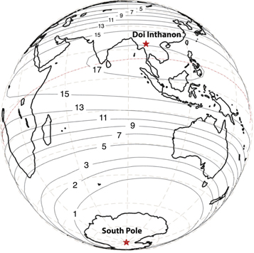
Figure 1. Contour plot of effective vertical geomagnetic cutoff rigidity in GV for part of Earth, also indicating the NM stations considered in this work, at Doi Inthanon, Thailand, with the world's highest effective vertical cutoff rigidity of 16.7 GV at altitude 2560 m, and at the South Pole, with a low geomagnetic cutoff and altitude 2820 m. Note that for a low geomagnetic cutoff (≲1 GV), the NM response to cosmic-ray ions is mainly determined by an atmospheric cutoff at ∼1 GV.
Download figure:
Standard image High-resolution imageThe ratio of count rates of NMs at different cutoff rigidity may provide an indication of spectral variations of cosmic rays. In practice, such a ratio does not achieve the precision expected for NM data because of different time-dependent systematic effects at different stations (see Figure 1 of Ruffolo et al. 2016). Indeed, such effects make it difficult to use such a ratio to infer spectral variations over short timescales of ≲1 month. Over long timescales, another concern is that the geomagnetic cutoff at some NM stations varies substantially with time (see Figure 1 of Mangeard et al. 2018). Furthermore, comparisons between NM stations can only provide spectral information within the range of cutoff rigidities of such stations, i.e., from ∼1 to 17 GV.
To avoid the systematic effects of comparing data from different stations, recent work has made use of neutron time-delay histograms from specialized electronics to provide some spectral information from a single NM. Initial results were obtained from a shipborne NM performing a latitude survey (Bieber et al. 2004), and similar methods were explored by other research groups (Balabin et al. 2008; Kollár et al. 2011; Krüger et al. 2017). Since 2007 December, such electronics have been used and further developed for the Princess Sirindhorn Neutron Monitor (PSNM) at Doi Inthanon, Thailand, which has the world's highest effective vertical cutoff rigidity for a fixed station (16.7 GV). (Note, however, that the cutoff depends on the arrival direction, so it actually occurs over a range of rigidities around ∼17 GV; see Appendix E for details.) The effect of chance coincidences has been statistically removed from the time-delay distribution to extract the "leader fraction," L, of neutrons that did not follow another neutron associated with the same primary cosmic ray (Ruffolo et al. 2016). Note that L corresponds to the inverse multiplicity of observed neutrons from the same cosmic ray and serves as an indicator of the spectral index of cosmic rays above the cutoff rigidity, as was confirmed using time-delay histograms from latitude surveys during 2001–2007 (Mangeard et al. 2016a). By providing information above the world's highest cutoff rigidity, the measurements of L at Doi Inthanon extend the rigidity range of spectral information from the worldwide NM network.
Here we report on the measurement of L at Doi Inthanon from 2007 December 9 to 2018 April 19 based on the continued development of electronic firmware and computer software to record time-delay histograms. While previous work examined short-term GCR spectral variations in data up to 2014 June 11 (Ruffolo et al. 2016), in the present work, we examine solar modulation of the GCR spectrum, which requires cross-calibration for different versions of firmware, software, and hardware to accurately normalize L for over 10 yr. In addition to measuring L at Doi Inthanon with the world's highest cutoff rigidity, these electronics were also installed at the South Pole NM with a low atmosphere-limited cutoff, and we report measurements there from 2013 December 10 to 2018 April 19. We also developed new or improved corrections to L for variations in atmospheric pressure and water vapor. Finally, we compare variations in the leader fraction L and count rate C. At both stations, to first approximation, L roughly tracked C, indicating GCR spectral variations due to solar modulation and Forbush decreases. At the South Pole, we also observed changes in L during 27 day variations with the Sun's rotation and one ground-level enhancement due to a solar storm. For data from Doi Inthanon that span the most recent solar magnetic polarity reversal, we find a hysteresis in L versus C that implies a difference in the GCR spectral shape above ∼17 GV due to solar modulation before or after the polarity reversal.
2. Neutron Time-delay Observations
2.1. PSNM at Doi Inthanon
Our techniques to examine GCR spectral variations using time-delay observations were mainly developed using data from PSNM at the summit of Doi Inthanon, Thailand's highest mountain, with geographic coordinates 18 59 N, 9849 E and altitude 2560 m. The PSNM has taken data since 2007 August, and since 2007 December 9, it has operated with a complete set of 18 BP-28 (10BF3) neutron-sensitive proportional counter tubes with the standard NM64 configuration (18NM64). The 18 tubes are arranged in a single row to reduce edge effects. Further details are available from Ruffolo et al. (2016).
We analyze time-delay observations from 2007 December 9 to 2018 April 18. During theat 10 yr period, we made various changes to PSNM firmware, software, and hardware. Based on these, the data were divided into nine normalization periods, DI-1 to DI-9. Details of changes in the data acquisition system and normalization periods can be found in Appendix A.
2.2. South Pole NM
Electronic firmware to record time-delay histograms has also been deployed at the South Pole NM. This is located at an altitude of 2828 m. It effectively comprises three 1NM64 detectors, each in a separate temperature-controlled outdoor box, using an 3He neutron-sensitive proportional counter tube. Details of changes in firmware and software in the data acquisition system used to collect time-delay histograms from the South Pole NM, as well as the four normalization periods SP-1 to SP-4, are provided in Appendix B.
2.3. Other NMs
Although we do not analyze other data in the present work, for completeness, we point out that these specialized electronics to collect time-delay histograms have been deployed on other NMs. They were first deployed with a shipborne 3NM64 for latitude surveys during 2000–2007, as analyzed by Mangeard et al. (2016a). More recently, they have been deployed on some of the counter tubes at the following NM stations: McMurdo, Antarctica (from 2015 until its closure in 2017); Newark, USA (since 2015); and Jang Bogo, Antarctica (since 2015). They were also deployed on two shipborne NM latitude surveys in 2019 and 2019–2020, and we plan to deploy them at the NM at Mawson, Antarctica, in 2020. In future work, these data should be analyzed to provide a more detailed picture of GCR spectral variations.
3. Leader Fraction Analysis
3.1. Extraction of the Leader Fraction
The leader fraction L is defined statistically as the fraction of neutron counts that did not follow another count in the same tube due to the same primary cosmic ray, i.e., did not follow another count in the same tube with a short time delay that is not consistent with chance coincidence. More energetic primary cosmic rays lead to more energetic secondary particles that produce more neutrons when interacting inside the NM (typically in the lead producer), which can then be detected as sequences of more counts in the same tube with shorter time delays. Thus, a harder cosmic-ray spectrum with a lower spectral index leads to a lower leader fraction.
In this work, we used the exponential tail fit parameters from the time-delay histogram, which Ruffolo et al. (2016) described as their first method to statistically measure chance coincidences and determine L. These values differ mainly due to each tube's position and electronic dead time (for details, see Mangeard et al. 2016b; Ruffolo et al. 2016). For the PSNM, tubes T1 and T18 at the edges of the row of 18 counter tubes have a lower value of L than the middle tubes, because the middle tubes have a larger fraction of neutron counts from interactions of atmospheric secondary particles in lead rings around neighboring tubes, leading to a lower neutron multiplicity at the tube of interest and a higher leader fraction. The variation of L from all counter tubes clearly shows a yearly wave, which can be attributed to the yearly variation in water vapor and atmospheric pressure (see Appendix A).
The 600 series firmware recorded time delays for only 16 pulses s–1, while the count rate in the 18NM64 at Doi Inthanon is ≈34 Hz per tube and that at the South Pole is ≈100 Hz per tube, resulting in poorer statistics and a "first-pulse bias" in the time-delay distribution. All L values from 600 series firmware were corrected for the first-pulse bias in the manner described by Ruffolo et al. (2016). The 700 and 800 series firmware record almost all time delays, so the first-pulse bias was negligible for such data.
Another issue before we determine L from the time-delay histograms is the overflow in the electronic recording system. For the 600 and 700 series firmware, the time delay was recorded modulo to = 142 ms, and we derived L from the following formula (Ruffolo et al. 2016):

where α and A are the parameters from fitting  to the exponential tail of the normalized measured histogram of time delay t, and td is the effective electronic dead time. When the time delays were calculated by the data acquisition software for the 800 series, a count was excluded from the histogram when the time delay was larger than to. Hence, for the 800 series firmware, we can use Equation (1) without the overflow correction:

normalizing the histogram to account for missing values at t > to.
3.2. Corrections for Atmospheric Pressure and Water Vapor
It is well known that any NM count rate is affected by variations in the atmospheric pressure, P, which serves as a proxy for the overlying airmass. This is due to energy-dependent absorption of secondary neutrons by the atmosphere, so it is unsurprising that the leader fraction L has been found to vary with P as well. Furthermore, previous work inferred that atmospheric water vapor pressure strongly affects the count rates of bare neutron counters at multiple locations and L at Doi Inthanon (Rosolem et al. 2013; Ruffolo et al. 2016). Water vapor even has a small but noticeable effect on the PSNM count rate C at Doi Inthanon, with a peak-to-peak seasonal variation of 0.3% (Mangeard et al. 2018). In this section, we discuss our techniques to correct both C and L as measured at Doi Inthanon and the South Pole for variations in P and (for Doi Inthanon) water vapor pressure.
For the PSNM at Doi Inthanon, it is possible to distinguish the effects of P and water vapor pressure. While both exhibit a yearly (seasonal) variation, there are also strong 12 and 24 hr variations in P due to atmospheric tides. In contrast, water vapor pressure is usually relatively constant over small timescales, and when it does vary rapidly, C and L do not exhibit corresponding variations, as will be discussed shortly. Because the South Pole is an extremely dry location (precipitable water vapor (PWV) typically below 1 mm), the effect of atmospheric water vapor is negligible, and we only correct for variations in P.
First, we focus on the effect of pressure variations, which result in anticorrelated variations in C and correlated variations in L. For C of either the PSNM or the South Pole NM, we use the standard barometric correction developed previously, by which C is multiplied by ![$\exp \left[\beta (P-{P}_{0})\right]$](https://content.cld.iop.org/journals/0004-637X/890/1/21/revision1/apjab6661ieqn2.gif) , where β is a pressure coefficient (0.641% hPa−1 for PSNM and 0.740% hPa−1 for the South Pole) and P0 is a reference pressure (750.5 hPa for PSNM and 680.0 hPa for the South Pole).
, where β is a pressure coefficient (0.641% hPa−1 for PSNM and 0.740% hPa−1 for the South Pole) and P0 is a reference pressure (750.5 hPa for PSNM and 680.0 hPa for the South Pole).
The leader fraction L is quite sensitive to the energy of secondary nucleons (see Figure 10 of Mangeard et al. 2016a), with a much lower L value (higher multiplicity) for GeV-range nucleons that typically originated in the upper atmosphere after at most a few GCR-induced interactions. With increasing atmospheric pressure, GeV-range nucleons are less likely to survive, and L increases. To observationally determine the effect on L, we fit data of  versus ΔP to straight lines of slope bi for each tube i. (Note: Given that the pressure has a positive correlation with L, in contrast with the negative correlation with C, to avoid confusion, we use the quantity b = −β for the pressure correction of L.) A quantity labeled by Δ refers to the residual with respect to a running average, i.e., a short-term fluctuation. For the PSNM, we use an hourly value minus a 24 hr average, so as to examine the effect of short-term P fluctuations, effectively filtering out the effects of water vapor and more gradual variations in the GCR flux. At the South Pole NM, the pressure mainly varies over ∼1 month (and the water vapor effect is negligible), so we use an hourly value minus a 30 day average.
For a given type of firmware, the b values for different counter tubes had minor variations with no clear dependence on the tube position or electronic dead time, so we use the mean value b for all counter tubes. For the PSNM, b for the 800 series firmware (0.0193% hPa−1) was higher than that for the 700 series (0.0154% hPa−1). Because of the similarities between the 600 and 700 series firmware, while L is determined with better statistical accuracy for the latter, we used b from the 700 series for the 600 series as well. For the South Pole NM, b for the 800 series was 0.0191% hPa−1, and that for the 600 series was 0.00922% hPa−1. Once we determined a value of b for the relevant firmware, then L was corrected for pressure variation by multiplying by ![$\exp \left[-b(P-{P}_{0})\right]$](https://content.cld.iop.org/journals/0004-637X/890/1/21/revision1/apjab6661ieqn4.gif) .
.
Next, let us examine the relationship between atmospheric water vapor and pressure-corrected C and L from Doi Inthanon. Because the effect of water vapor on C is much smaller and, over subannual timescales, is difficult to distinguish from the effect of a changing GCR flux, we analyze the effect on L and expect that the effect on C should be qualitatively similar. Note that previous work found a nonlinear relationship between the surface water vapor pressure Ew and pressure-corrected L, where Ew was derived using data of relative humidity and temperature from the Global Atmospheric Data Assimilation (GDAS) database,7 interpolating values from the four surrounding degree-scale spatial grid points to the geographic location of the PSNM, for a pressure level close to the reference pressure at the summit of Doi Inthanon (Ruffolo et al. 2016). The nonlinear relationship is consistent with a saturation of surface water vapor during the rainy season (roughly from April through October), while the effect of water vapor on L continues even as Ew saturates. Note also that Mangeard et al. (2018; see their Figure 2) modeled the effect of Ew on the count rate C using a linear relationship; however, the effect on C is quite small, as noted above, so a possible nonlinearity would be difficult to measure.
Physically, it seems more reasonable that L is affected by water vapor throughout the atmosphere (hence the continued effect on L as the surface water vapor pressure Ew saturates), and that the effect of the total atmospheric water vapor should be linear. Therefore, we used GDAS data to determine the PWV at Doi Inthanon, i.e., the height of liquid water (in mm) that would result if all of the water vapor in the atmosphere were to condense at the surface, to determine whether this would provide a more reasonable model for the water vapor effect on L. The PWV was determined by numerically integrating the water vapor pressure for the atmosphere above Doi Inthanon as inferred from GDAS data, which have a 6 hr cadence. The PWV for the entire period of PSNM data can be found in Appendix A.
Figure 2 shows scatter plots of the pressure-corrected L averaged over all 18 counter tubes with 24 hr smoothing (to reduce the statistical uncertainty) versus (a) Ew and (b) PWV, with the 6 hr cadence of the GDAS data, for the normalization period DI-2 (with 700 series firmware) from 2011 January 15 to 2014 February 8. This time period was chosen because of the good statistical quality provided by 700 series firmware, the constant configuration for 3 yr (see Appendix A), and the nearly constant level of solar modulation for the PSNM at this time (Mangeard et al. 2018), so that time variations in L can mostly be attributed to the water vapor effect, except for occasional Forbush decrease effects that are unrelated to the water vapor pressure. It can be seen that the relationship with Ew is nonlinear, in agreement with Ruffolo et al. (2016), while the relationship with PWV is apparently linear. Presumably, this is due to moderation and absorption of low-energy atmospheric secondary neutrons by water vapor throughout the atmosphere. Thus, a higher PWV can lead to a lower fraction of low-energy secondary neutrons, a higher average multiplicity, and a lower leader fraction. The surface water vapor Ew can serve as a proxy for PWV but often saturates during the rainy season (with nearly 100% relative humidity) so that L has a nonlinear relationship with Ew. In that case, PWV should provide a more direct measure of water vapor content for correcting L and C from the PSNM.
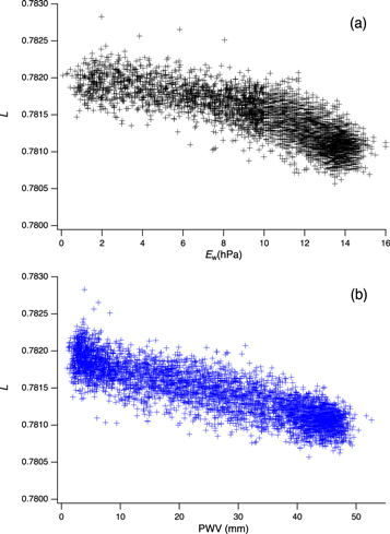
Figure 2. Scatter plot of the tube-averaged pressure-corrected leader fraction L from the PSNM with 24 hr smoothing as a function of (a) surface water vapor pressure Ew and (b) PWV at Doi Inthanon as inferred from the GDAS database, with a 6 hr cadence for the time period DI-2 (2011 January to 2014 February). These plots indicate a nonlinear relationship between L and Ew and a linear relationship with PWV, from which we infer that PWV has a closer physical relationship with L.
Download figure:
Standard image High-resolution imageFigure 3 shows PSNM data of C, L, and PWV as a function of time for the same time period (DI-2). For C and L, the gray line indicates daily tube-averaged values that are corrected for pressure but not yet for water vapor, while in Figure 3(c), the blue line indicates PWV determined from GDAS data with a 6 hr cadence. Note that there are some relatively sharp decreases in L in association with changes in C, reflecting the effect of GCR spectral and flux variations, respectively. For example, there are sharp Forbush decreases in C (Forbush 1937) associated with the passage of a shock or possibly the ejecta from a solar storm, such as those on 2012 March 8 and 12, and some Forbush decreases are also associated with decreases in L, i.e., GCR spectral variations above the ∼17 GV cutoff (Ruffolo et al. 2016).
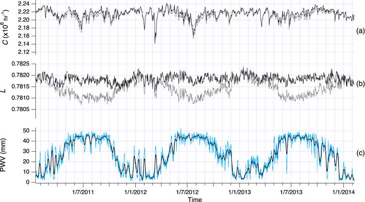
Figure 3. (a) Daily count rate C and (b) leader fraction L from the PSNM during time period DI-2 for 700 series firmware as corrected for pressure (gray) and for pressure and PWV (black). (c) The PWV as determined from the GDAS database, at a 6 hr cadence, without (blue) and with (black) triangular smoothing to ±5 days. Our correction for PWV mostly removes a seasonal wave from the C and L data, allowing a clearer measurement of variations in the cosmic-ray flux (from C) and the cosmic-ray spectral index (from L) for rigidities above the ∼17 GV cutoff at Doi Inthanon.
Download figure:
Standard image High-resolution imageThe remaining nonstatistical variations in L are closely but not perfectly associated with variations in PWV. In addition to the large seasonal wave, L also varies according to shorter-term variations in PWV. Some clear changes in L of this type, while C was nearly constant, occurred from late 2011 December to early 2012 January and during 2013 October. These were associated with changes in PWV that lasted ≳10 days and provide convincing evidence of an association of L with atmospheric water vapor as opposed to another seasonal variation. However, L does not exactly follow more rapid changes in PWV as determined from GDAS. For example, during the rainy season in 2013 June, there was a sharp decline of PWV to a dry-season level, followed by a rapid recovery back to a nearly maximal level. At that time, there was only a small change in L, nowhere near the dry-season level. If we were to correct L based directly on this PWV time series, that would induce spurious spikes in L from overcorrection of shorter-term PWV variations that do not have a proportional effect on L.
We have solved this problem by smoothing the GDAS-derived PWV time series for use in correcting the leader fraction. After testing smoothing of various types and durations, we found a good correspondence between variations of LPcorr (as corrected for pressure but not water vapor variations) and those of PWV smoothed with a triangular function that peaks at the actual time and goes to zero over ±5 days. This 10 day triangle-smoothed GDAS-derived PWV time series is shown as the black curve in Figure 3(c) and can be visually seen to be better anticorrelated with the vapor-uncorrected leader fraction (gray) in Figure 3(b) during times of nearly constant C.
To confirm that GDAS provides a useful description of PWV, we compared PWV as determined from GDAS data with PWV determined in other ways. For example, we determined PWV from another database, the Modern-Era Retrospective Analysis for Research and Applications, Version 2 (MERRA-2),8 during 2013. This comparison was quite interesting, as the two values of PWV agreed very well at most times, with a correlation coefficient r2 = 0.933, but occasionally sharp features were different or occurred with a time difference of up to 4 days in the two databases. This implies that there can be a temporal uncertainty in the use of such databases to infer the time profile of PWV. Another comparison was with direct measurements from a radiosonde on balloons launched daily at the airport in Chiang Mai, Thailand, which is located 55 km from Doi Inthanon at an elevation of about 300 m above sea level. We compared PWV inferred from the radiosonde and GDAS data for that location during 2013 January–October and found a very good correspondence between the two (r2 = 0.926). Finally, we operated a two-frequency GPS receiver at the PSNM site from 2017 November to 2018 June, determining the zenith time delay and subtracting the delay associated with the dry atmosphere to infer the PWV (Takiguchi et al. 2000). We used the techniques of Bevis et al. (1992), with the refinement of using the mean atmospheric temperature Tm as determined from the GDAS database instead of estimating this from the surface temperature. The PWV values obtained from the GPS data had a different absolute normalization, nearly 40% lower than the PWV from GDAS, but the values from GPS and GDAS data were very well correlated (r2 = 0.953).
These comparisons give us confidence that GDAS provides a useful measure of PWV. However, the comparison with PWV from MERRA-2 indicates that PWV features can appear at different times when using different databases. This could be partly attributed to our bilinear interpolation of data from the four nearest 1° grid points, which could make features appear at times when, in reality, the feature was not occurring at Doi Inthanon. This could be a reason why temporal smoothing of the inferred PWV is required to better match the actual effects on L. Another possibility is that PWV is in part a proxy for rainwater on or in the concrete and rock surfaces surrounding the PSNM building. (Note that the building itself has a roof slanted at 45° that does not accumulate rainwater; see Figure 1(a) of Ruffolo et al. 2016.) However, we tested pouring water onto these surfaces on two occasions for up to several hours and were unable to detect a change in PSNM data. Furthermore, the effect of rainwater should lead to a time delay, whereas when we tried different smoothing profiles, a delayed profile provided no better results than the symmetric profile that we adopted. For these reasons, we view the need for temporal smoothing as best attributed to temporal uncertainties in our determination of PWV.
To correct L for the effect of water vapor, we performed linear fits to LPcorr after 24 hr smoothing versus the 10 day triangle-smoothed PWV calculated from GDAS data with a 6 hr cadence separately for each tube and series of firmware. Then the leader fraction corrected for pressure and water vapor is determined as

where a is the negative slope divided by the intercept of the linear relationship. The reference value PWV0 = 7.2 mm is the median value of PWV in January, during the dry season. The PWV at the PSNM varies from as low as 1 mm in the dry season to a maximum of ≈55 mm in the rainy season.
For a given firmware series, the value of a was quite different between the two end counter tubes and the 16 middle counter tubes, so we used average values for either the end or middle tubes. The values of a for the 700 series firmware were 2.635 × 10⁻⁵ mm−1 for the middle tubes and 3.685 × 10⁻⁵ mm−1 for the end tubes. These are higher than the values for 800 series firmware, which are 2.412 × 10⁻⁵ mm−1 for the middle tubes and 3.221 × 10⁻⁵ mm−1 for the end tubes. As with the pressure correction, for the 600 series firmware, we used the same values of a as for the 700 series firmware.
The leader fraction after vapor correction (black) in Figure 3(b) does not appear to contain spurious short-term spikes due to over- or undercorrection. There are still some systematic variations over scales of months that are not associated with cosmic-ray flux variations as indicated by the count rate C, such as during 2011 December and 2013 January, when C was nearly constant at ≈2.2 × 10⁶ hr−1. Over such times, the pressure- and vapor-corrected L varied from about 0.7816 to 0.7822. We conclude that our vapor correction involves a residual systematic error in L of up to 3 × 10⁻⁴. By averaging L over 3 month intervals, we can reduce that systematic error, as well as statistical errors.
Mangeard et al. (2018) reported a peak-to-peak annual variation of 0.3% in the pressure-corrected count rate, which is attributed to a water vapor effect, compared with the total peak-to-peak solar modulation of ≈3%, so the effect of water vapor is nonnegligible. Our procedure to correct this effect on C is slightly different than for L, because C mostly varies due to true variations in the cosmic-ray flux, e.g., due to Forbush decreases and solar modulation. Therefore, we follow a procedure similar to that of Mangeard et al. (2018), using PWV in place of the surface water vapor pressure Ew. For various ranges of the 10 day triangle-smoothed PWV (bins of 5 mm each), we calculated the median value over 2007 December to 2018 April of the pressure-corrected count rate summed over all 18 counter tubes, CPcorr. The median is used in order to reduce the effects of outlier values due to short-term cosmic-ray flux variations. Then we performed a linear fit to the median values of CPcorr versus the smoothed PWV. Finally, the count rate corrected for pressure and water vapor is evaluated as

where a is found from the negative slope divided by the intercept of the linear fit to be (10.18 ± 2.41) × 10−5 mm−1. For time period DI-2, Figure 3(a) shows CPcorr (gray) and CPWcorr (black). The latter, corrected for pressure and water vapor variations, is now seen to have the seasonal variation effectively removed, revealing a nearly constant GCR flux punctuated by sporadic Forbush decreases due to solar storms.
After correction for atmospheric effects, it was necessary to normalize L to account for differences among counter tubes, firmware versions, some software versions, and hardware. Details can be found in Appendix C for the PSNM and Appendix D for the South Pole NM. The resulting time series of C and L at Doi Inthanon are shown in Figure 4. Those at the South Pole are shown in Figure 5, where the leader fraction data from 2013 December to 2014 November are plotted in blue to highlight their uncertain normalization relative to later data (in black; see Appendix D for details).
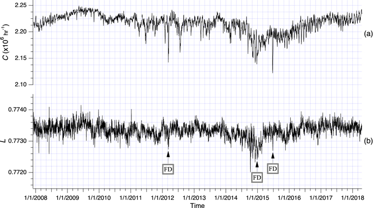
Figure 4. Daily averaged data of the pressure- and vapor-corrected (a) count rate C and (b) leader fraction L vs. time after normalization for the 18NM64 at Doi Inthanon at a cutoff rigidity of ∼17 GV during 2007 December–2018 April. Variations in C and L indicate changes in the cosmic-ray flux and spectral index, respectively, for a rigidity range above the local cutoff. The long-term time variation is due to solar modulation of the cosmic-ray spectrum. Note that sunspot minimum occurred in 2009, and sunspot maximum occurred in 2014. Selected Forbush decreases are indicated by "FD."
Download figure:
Standard image High-resolution image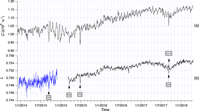
Figure 5. Daily averaged data of the pressure-corrected (a) count rate C and (b) leader fraction L vs. time after normalization for the 3 × 1NM64 at the South Pole at an atmosphere-limited cutoff rigidity of ∼1 GV during 2013 December–2018 April. Blue indicates an uncertain normalization of the data from 2013 December–2014 November relative to the later data. The long-term variation is due to solar modulation of the cosmic-ray spectrum. Selected Forbush decreases are indicated by "FD," and a ground-level enhancement is indicated by "GLE."
Download figure:
Standard image High-resolution image4. Spectral Variations of Cosmic Rays
4.1. Solar Modulation
Next, let us consider the variation of the count rate C and leader fraction L over the recent sunspot cycle from NMs at Doi Inthanon and (for a half-cycle) the South Pole. In each case, C measures the sum of the GCR differential response function (spectrum times NM yield function) for each species, integrated over rigidity above the cutoff (Simpson et al. 1953), i.e., for rigidity ≳17 GV at Doi Inthanon and ≳1 GV at the South Pole. Thus, variations in an NM count rate indicate variations in the GCR flux above the local cutoff. Similarly, for each station, variations in L indicate variations in the GCR spectral index over the rigidity range of the NM response, as shown by Mangeard et al. (2016a) for observations and Monte Carlo simulations of L during a series of NM latitude surveys.
Figure 6 shows 3 month averaged data for the leader fraction L versus count rate C over the whole time period of analysis from Doi Inthanon. The data are averaged over 3 months to reduce the systematic uncertainty from the water vapor correction and the statistical uncertainty. The number at each point indicates the order of the 3 month period, starting with 1 for 2007 December–2008 February and ending with 42 for 2018 March–April (truncated to 2018 April 19 when our analysis ends). One way to estimate the uncertainty of L after the 3 month averaging is to consider the coherence time of the fluctuations. The statistical fluctuations seen in Figure 4 are independent from day to day, so after averaging over 3 months, they are reduced by a factor of about  , making the statistical uncertainty much smaller than the systematic uncertainty. Section 3.2 reported a systematic effect due to imperfect correction for the effect of atmospheric water vapor, with a maximum deviation of 0.0003. This maximum is rarely reached, and we estimate the standard deviation to be about 0.0002. Based on Figure 3, focusing on times when C was nearly constant, so changes in L due to GCR spectral variations should be small, the coherence time of these fluctuations is estimated as about 0.5 months. Therefore, a 3 month average contains about six independent samples of such fluctuations, so the standard error is a factor of
  lower than the standard deviation of the fluctuations (0.0002). We conservatively estimate the uncertainty in the 3 month averages of L from the PSNM as 0.0001. Another way to estimate this is to simply examine the scatter among L from neighboring intervals in Figure 6, which confirms an uncertainty of about 0.0001.
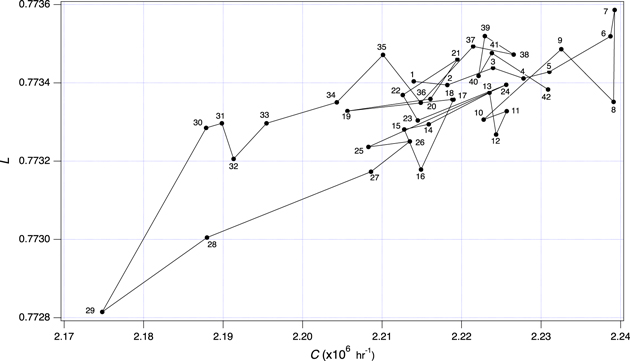
Figure 6. Trimester (3 month) averages of the leader fraction L vs. count rate C from Figure 4 for the 18NM64 at Doi Inthanon during 2007 December–2018 April. Labels indicate the time period, starting at 1 for 2007 December–2008 February and ending at 42 for 2018 March–April. The hysteresis indicates that for solar modulation above the ∼17 GV cutoff over the recent sunspot cycle, the cosmic-ray spectrum did not roll down and unroll back up in the same way. Apparently, there was a change in the nature of the solar modulation around the time of the solar magnetic polarity reversal that occurred near sunspot maximum, even at this high rigidity range.
Download figure:
Standard image High-resolution imageFigure 7 shows monthly averaged data for L versus C from the South Pole. Although the total count rate is ≈1.1 × 10⁶ hr−1 compared with ≈2.2 × 10⁶ hr−1 for Doi Inthanon, the South Pole data are not affected by water vapor with an associated systematic uncertainty, and the total variation of L over the solar cycle is much greater, i.e., about 6 × 10⁻³ for the South Pole compared with 8 × 10⁻⁴ for Doi Inthanon. For these reasons, the monthly L data from the South Pole provide useful data for studying solar modulation, currently for half a solar cycle. The numbers in Figure 7 start at 1 for 2013 December and end at 53 for 2018 April.
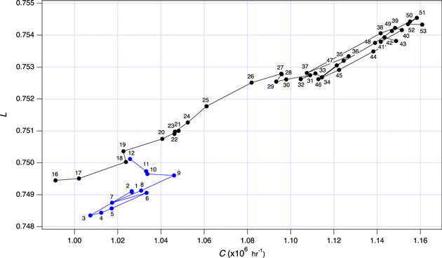
Figure 7. Monthly averages of the leader fraction L vs. count rate C from Figure 5 for the 3 × 1NM64 at the South Pole during 2013 December–2018 April. Labels indicate the order of monthly data points, starting at 1 for 2013 December and ending at 53 for 2018 April. Blue indicates an uncertain normalization of the data from 2013 December to 2014 November relative to the later data, which show a nearly linear relationship between L and C for a half-cycle of solar modulation.
Download figure:
Standard image High-resolution imageA basic concept of solar modulation is that with increasing solar activity, the cosmic-ray spectrum "rolls" downward from the local interstellar spectrum, and with decreasing solar activity, the spectrum "unrolls" upward again. The change in flux is much greater at low rigidity, while at sufficiently high rigidity, there is almost no solar modulation (Rao 1972). Thus, we expect that as C decreases, L will also decrease. If the GCR spectral shape were the same during the rolling and unrolling, e.g., as in the force-field model of solar modulation, then L versus C would follow the same path during downward and upward trajectories.
For the South Pole NM, the normalization of the initial data for L during SP-1 (2013 December to 2014 November) relative to later data is uncertain (as explained in D), as indicated in blue in Figure 7. After a 3 month data gap (corresponding to the missing numbers 13–15), the data from 2015 March (point 16) to 2018 April (point 53) follow a consistent, nearly linear trend. This is consistent with the "unrolling" of the GCR spectrum in the 1–10 GV range that dominated the variation in South Pole data with solar modulation as solar activity weakened.
For the PSNM at Doi Inthanon, recording L and C over a full solar cycle, we observe a hysteresis loop, implying a change in the GCR spectral shape above the cutoff rigidity of ∼17 GV. In other words, the GCR spectrum had a different shape in this high rigidity range while rolling down and unrolling back up again. Note that the time period of declining cosmic-ray flux was associated with solar modulation from the A < 0 phase of the solar cycle (i.e., with a mostly inward magnetic field at the northern hemisphere of the Sun) as its effects propagated through the heliosphere, and the rising cosmic-ray rate was associated with the A > 0 phase. Thus, our results imply a change in spectral shape with a change in solar magnetic polarity at a rigidity range above the ∼17 GV cutoff.
Such changes have been reported from comparisons between NM measurements at different locations with different cutoff rigidity (Moraal et al. 1989; Nuntiyakul et al. 2014; Mangeard et al. 2018), a technique that is limited to the Earth's range of atmospheric and geomagnetic cutoff rigidities, ∼1–17 GV. In this work, we find distinct changes in the evolution of the cosmic-ray spectral shape at P ≳ 17 GV during periods of opposite solar magnetic polarity, as detailed below.
During 2007 December to 2015 February (points 1–29 in Figure 6), C and L at Doi Inthanon first increased and then declined along a roughly linear trend, which is again consistent with the rolling of the spectrum with greater variation at lower rigidity, so that the spectral index decreased (hardened) along with the count rate decrease. This time period was mostly associated with A < 0 solar magnetic polarity (Mangeard et al. 2018). However, shortly after the cosmic-ray minimum in early 2015, now with A > 0 solar magnetic polarity, L shot upward to a nearly maximal value while C increased only slightly, a qualitatively different pattern from that observed at the South Pole. This implies little change in the count rate while the spectral index above the cutoff rapidly increased, indicating a rapid recovery of the GCR flux at about 17 GV, while the flux at higher energy had little or no increase or perhaps even declined to result in the nearly constant count rate. This was a significant reorganization of the GCR spectrum above ∼17 GV within a short time period in early 2015.
From 2015 March to 2018 April, the count rate at Doi Inthanon mostly had a gradual increase (punctuated by sharp 27 day variations), while the L and spectral index remained nearly constant, in contrast with the behavior during 2007–2014 in the A < 0 phase of modulation. The nearly constant spectral index after early 2015 implies a nearly rigidity-independent increase in the flux over a significant rigidity range above the cutoff.
4.2. Relationship between the Leader Fraction and a Spectral Index
We have noted that the leader fraction L serves as an indicator of the GCR spectral index, so it is interesting to estimate a relationship between the two. This leads to the question: what is the rigidity (or energy) for which L indicates the spectral index? For the PSNM, the median primary GCR rigidity is 35 GV, and the 10th–90th percentile range of its response is from 18 to 155 GV (Ruffolo et al. 2016). However, solar modulation has a very low effect on the higher rigidities in that range. Based on measurements by the AMS-02 detector on the International Space Station over the time period of 2011 May to 2013 November (Aguilar et al. 2015a, 2015b), we see that the primary cosmic-ray spectral index was roughly independent of rigidity above 40 GV (within the uncertainties), which could indicate that solar modulation has little effect at P > 40 GV and hardens the spectrum at lower rigidity. This view is supported by AMS-02 measurements indicating little or no time variation in the proton flux at 41.9–45.1 GV from 2011 May to 2017 April (Aguilar et al. 2018). Therefore, we estimate that the variation of L at Doi Inthanon due to solar modulation mainly reflects the variation of the GCR spectral index over ∼20–40 GV. For a polar NM, the response includes a very wide range of rigidity over which solar modulation has strong effects, and the spectral index strongly varies with rigidity, so we do not attempt to relate L at the South Pole NM to a spectral index over a specific rigidity interval.
Even for the PSNM, estimating the relationship between L and a spectral index over ∼20–40 GV brings up further questions. What spectral form should we assume? Can the variation of the GCR spectrum above ∼20 GV due to solar modulation be characterized by varying a single parameter? The second question is clearly answered by our discussion in the preceding subsection: solar modulation of the GCR spectrum above the ∼17 GV cutoff at Doi Inthanon is not well characterized by a single parameter. This is clear from the hysteresis in Figure 6; different times with the same count rate can have different leader fractions, indicating a different spectral shape. Nevertheless, in order to provide a rough calculation of how changes in the spectral index over ∼20–40 GV correspond to changes in L, we have performed a calculation based on broken power-law spectra for protons and for ions with Z ≥ 2. The break in the power law is set at 40 GV. The power-law indices for >40 GV are fixed at values based on results from AMS-02 (Aguilar et al. 2015a, 2015b), while the power-law index γ<40GV for protons at <40 GV is allowed to vary (i.e., due to solar modulation) and the power-law index for Z ≥ 2 varies in tandem. We stress that we are not proposing this broken power law as a proper description of the GCR spectrum.
Appendix E explains how we obtained yield functions from Monte Carlo simulations and used the model spectrum described above to calculate  . Figure 6 indicates that the full variation of L over the past solar cycle was about 0.0008. This implies a variation in
  of ≈0.2 over the solar cycle, as measured over the rigidity range from the ∼17 GV cutoff at Doi Inthanon to ∼40 GV.
4.3. Other Variations
Previous work reported short-term spectral hardening as indicated by decreases in L from Doi Inthanon (Ruffolo et al. 2016) during Forbush decreases in C. These short-term decreases are associated with solar storms (Forbush 1937), in particular, the passage of a coronal mass ejection and/or an associated shock (Cane 2000). The decrease is stronger at lower rigidity, hence the spectral hardening. Selected Forbush decreases are indicated in Figures 4 and 5. These are times when C and L decrease very rapidly (typically for ≲1 day) and recover (increase) to near their prior levels for up to several days. Figure 4 confirms decreases in L (spectral hardening) at Doi Inthanon to various degrees for the stronger Forbush decreases in the past solar cycle.
In Figure 5, we see decreases in L much more clearly in data from the South Pole NM at times of Forbush decreases in C. As noted earlier, variations in L are clearer at the South Pole because GCR variations are stronger at low cutoff rigidity, and also because the South Pole is a very dry location where there is no water vapor effect or associated systematic uncertainty.
Figure 5 also exhibits a sharp increase in L on 2017 September 10. This is associated with the ground-level enhancement on that day (Kurt et al. 2018), as indicated in the figure, due to a solar storm that produced a sufficiently high flux of relativistic solar particles that there was a measurable flux enhancement over the GCR flux, especially at low cutoff rigidity, due to the much softer spectrum of solar particles. Interestingly, the ground-level enhancement is more clearly visible in the leader fraction L than in the count rate C, indicating that spectral signatures can assist in the detection of ground-level enhancements that involve only a weak count rate enhancement.
A noteworthy feature of C versus time at both Doi Inthanon and the South Pole (in Figures 4 and 5) is the 27 day variation (Fonger 1953), which was particularly prominent from late 2014 to 2018. This varies with the 27 day period of solar rotation, because the solar wind speed depends on the source location at the Sun. In particular, there can be high-speed solar wind streams in interplanetary space that collide with the preceding slower solar wind to form corotating interaction regions (e.g., Hundhausen et al. 1980), and these corotating features can be associated with recurrent decreases in the GCR flux. In the data for L at the South Pole, for the first time, we can confirm 27 day variations in L together with those in C. The implied spectral hardening during recurrent decreases in C is again expected because the 27 day features are fractionally stronger at lower rigidity (Gil & Alania 2010).
Note that in Figures 4 and 5, C and L are plotted to show the variations with solar modulation on a similar scale. With this scale, the shorter-term variations in L are much smaller than the variations in C. In other words, variations in L relative to the 27 day variations and Forbush decreases in C are much weaker than those for solar modulation. This indicates that the physical processes causing such variations do not roll and unroll the cosmic-ray spectrum as strongly as solar modulation. In other words, 27 day variations and Forbush decreases are not as strongly enhanced at low rigidity as solar modulation.
5. Summary
We have used specialized electronics to collect neutron time-delay histograms from two high-altitude NM stations that detect neutrons from atmospheric showers of cosmic rays. These are the PSNM at Doi Inthanon, Thailand (altitude 2560 m), the station with the world's highest effective vertical cutoff rigidity of 16.7 GV, and the NM at the South Pole (altitude 2820 m), with a low atmosphere-limited cutoff of ∼1 GV. From the time-delay histograms, we used the methods of Ruffolo et al. (2016) to statistically extract the leader fraction, L, i.e., the fraction of counts that did not follow temporally associated neutron counts in the same counter tube from the same primary cosmic ray. Here L measures the inverse multiplicity of neutrons in the counter tube, and variations in L are associated with variations in the GCR spectral index, avoiding the systematic errors from comparison of data from different NM stations. This work presents new results from Doi Inthanon over the past sunspot cycle and the South Pole over a half-cycle, including an improved correction for the effect of atmospheric water vapor variations at Doi Inthanon and normalization of L for changes in firmware, software, and hardware as we improved the collection of time-delay histograms.
Cosmic-ray variations are usually stronger at lower energy or rigidity, so to first order, we expect decreases in the NM count rate C, indicating the cosmic-ray flux above the local cutoff rigidity, to involve spectral hardening and simultaneous decreases in L. We do observe that C and L generally vary in the same direction. For the South Pole NM, solar modulation of GCRs over the recent sunspot half-cycle indeed leads to a similar pattern in C and L.
For the Doi Inthanon NM at a high cutoff rigidity, we observed different behaviors over the recent sunspot cycle. During the A < 0 solar magnetic polarity, C and L increased and decreased in tandem, indicating a gradual rolling of the GCR spectrum at ≳17 GV. After the sunspot maximum and solar polarity reversal, in early 2015, L rapidly shot up to nearly its solar minimum value, indicating a rapid reorganization of the GCR spectrum above ∼17 GV to a shape similar to that achieved near solar minimum, while the count rate C was only beginning to recover. That spectral shape was maintained as C rose to nearly solar near-minimum conditions in 2018 April.
Use of the leader fraction from the Doi Inthanon NM provides information about the cosmic-ray spectrum above the world's highest geomagnetic cutoff, thus extending the spectral reach of the worldwide cosmic-ray network. These precise measurements allow us to explore the details of solar modulation in a rigidity range above 17 GV that was previously inaccessible.
Meanwhile, the South Pole NM (with the advantage of a very dry climate) allows precise measurements of shorter-term spectral variations. We now observe 27 day variations in L associated with solar rotation, high-speed streams, and corotating interaction regions, and we observe an increase in L during a ground-level enhancement due to relativistic solar particles. We confirm dips in L along with Forbush decreases due to solar storms. Notably, the variations in L relative to the 27 day variations and Forbush decreases in C are much weaker than for solar modulation, indicating weaker changes in spectral shape. Continued measurements at Doi Inthanon and the South Pole, along with further deployment of the specialized electronics at other Antarctic stations, promise further detailed cosmic-ray spectral information using these techniques.
This work was partially supported by Thailand Science Research and Innovation award RTA6280002 and US National Science Foundation awards PLR/ATE-1341312, PLR-1245939, PLR-1341562, and their predecessors. We thank Charun Upara, Yanee Tangjai, Pornchai Supnithi, Jirapoom Budtho, and Pakkapawn Prapan for helping with the study of the effects of water vapor.
Appendix A: Changes in Data Acquisition at Doi Inthanon
Table 1 details the evolution of the firmware (microcontroller code) in the electronics and the software in the data acquisition system used to collect time-delay histograms at the PSNM. Normalization periods at Doi Inthanon (DI-1 to DI-9) are defined according to significant changes in firmware and/or software. (Note that none of these changes affected the separate circuitry used to record count rates, which were collected almost continuously from the 18NM64 since 2007 December 9). Figure 8(a) shows the leader fraction of each of the 18 neutron counter tubes as extracted from the time-delay histograms, using methods described in Section 3.1, and also indicates the start of each normalization period. All data from 600 series firmware have already been corrected for the first-pulse bias described in Section 3.1. In this figure, the data have also been cleaned to remove erroneous spikes but are otherwise not yet normalized or corrected for atmospheric effects. As pointed out by Ruffolo et al. (2016), the two end tubes have lower leader fractions than the middle tubes. These leader fraction data exhibit a seasonal wave, which we attribute to the effects of atmospheric pressure (Figure 8(b)) and water vapor (Figure 8(c)).
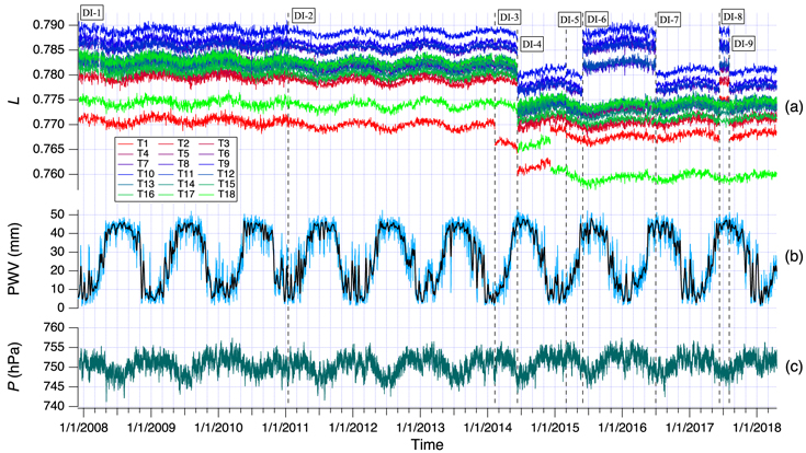
Figure 8. Time variations in daily averaged data for the PSNM at Doi Inthanon. (a) Uncorrected and unnormalized leader fraction L for all 18 counter tubes, indicating the start of each normalization period (DI-1 to DI-9) with significantly different firmware or software. Note that the two end tubes have lower L than the other tubes. See text for details. (b) PWV as determined from the GDAS database, without (blue) and with (black) triangular smoothing to ±5 days. (c) Atmospheric pressure P as measured at the PSNM. We find that both PWV and P affect the measured value of L, and we developed improved corrections for these atmospheric effects.
Download figure:
Standard image High-resolution imageTable 1. Time Periods of Neutron Time-delay Data Collection from the 18NM64 at Doi Inthanon
| Normalization | Start Date | End Date | Cadence | Firmware Series | Software Versiona |
|---|---|---|---|---|---|
| Period | (Number of Tubes) | ||||
| DI-1a | 2007 Dec 9 | 2009 Jun 28 | Daily | 600 (18) | ⋯ |
| DI-1b | 2009 Jun 29 | 2011 Jan 15 | Hourly | 600 (18) | ⋯ |
| DI-2 | 2011 Jan 15 | 2014 Feb 8 | Hourly | 700 (18) | ⋯ |
| DI-3 | 2014 Feb 8 | 2014 Jun 11 | Hourly | 700 (17) | ⋯ |
| DI-4a | 2014 Jun 11 | 2014 Dec 6 | Daily | 800 (18) | 8.34–8.46 |
| DI-4b | 2014 Dec 7 | 2015 Mar 3 | Hourly | 800 (18) | 8.47 |
| DI-5 | 2015 Mar 3 | 2015 May 29 | Hourly | 800 (18) | 8.50 |
| DI-6a | 2015 May 31 | 2016 May 17 | Hourly | 600 (6), 800 (12) | 8.50–8.82 |
| DI-6b | 2016 May 18 | 2016 Jun 30 | Hourly | 600 (6), 800 (12) | 8.82 |
| DI-7 | 2016 Jun 30 | 2017 Jun 12 | Hourly | 800 (18) | 8.82 |
| DI-8 | 2017 Jun 12 | 2017 Aug 3 | Hourly | 600(6), 700(6), 800(6) | 8.91–8.93 |
| DI-9 | 2017 Aug 4 | 2018 Apr 19 | Hourly | 800 (18) | 8.93–8.124 |
Note.
aOnly relevant for 800 firmware.Download table as: ASCIITypeset image
During DI-1, starting on 2007 December 9, we used the 600 series firmware to collect daily time-delay histograms from the 18NM64, and the software was changed to collect hourly histograms starting on 2009 June 29. The hourly cadence allows us to correct the data for atmospheric pressure variations on an hourly basis; at this near-equatorial location, the pressure has a strong 12 hr tidal period. The 600 series firmware is limited to collecting pulse heights and time delays (and recording them in histogram form) at only 16 Hz per tube, whereas the PSNM count rate is ∼34 Hz per tube. Therefore, during DI-2, starting on 2011 January 15, we used 700 series firmware that we developed to collect time delays at up to 48 Hz per tube, permitting a reduction of statistical uncertainty that is clearly visible in Figure 8(a).
On 2014 February 8, we started the process of upgrading to 800 series firmware on tube number 1, but this initial version of the firmware did not produce usable histograms, so for this time period (DI-3), we use only 700 series firmware on the remaining 17 tubes. On 2014 June 11, at the start of DI-4, we upgraded to new 800 series firmware (as currently used) in order to calculate absolute times and cross-tube time-delay histograms (Sáiz et al. 2017); the cross-tube histograms are not used in the present analysis. The 800 series firmware also reduced the time-delay dead time for improved collection of time-delay data; the reduced dead time is the main reason for the decrease in L as seen in Figure 8(a). For the 800 series, absolute time delays are calculated by the data acquisition software and therefore can depend on changes in the software version or computer used for data acquisition. During DI-4a, there were software issues that can be corrected with a daily cadence, followed by DI-4b when hourly values of L are obtained again. Note that on 2014 December 7, counter tubes 1 and 18 were swapped in order to study the effect of tube position (Mangeard et al. 2016b); the average leader fraction and count rate were unchanged. After new software was implemented on 2015 March 3, the normalization of L was slightly different during DI-5. We did not observe any difference in L associated with further changes in the software version.
Further changes were associated with calibration of the leader fraction by using different firmware on different tubes at the same time. During DI-6, which started on 2015 May 31 and ended on 2016 June 30, time-delay histograms were recorded from the 600 series on 6 counter tubes (T7–T12) and from the 800 series on the remaining 12 counter tubes. Afterwards, we changed the data acquisition computer on 2016 May 18 and found an increase in L from the 800 series from DI-6a before the change to DI-6b after the change. During DI-7, we restored the 800 series firmware to all counter tubes and used only one software version to record time-delay histograms. Then, during DI-8, we performed a second calibration with the 700 series on tubes 1–6, 600 series on tubes 7–12, and 800 series on tubes 13–18. The second calibration period ended on 2017 August 3, and afterward (during DI-9), we used the 800 series on all counter tubes, ending our analysis on 2018 April 19.
Appendix B: Changes in Data Acquisition at the South Pole
Table 2 lists normalization periods SP-1 to SP-4 corresponding to significant changes in the firmware and software used to collect time-delay histograms at the South Pole NM. Figure 9(a) shows the leader fraction for each of the three counter tubes, as well as the start of each normalization period. We can clearly see the effect of atmospheric pressure (Figure 8(b)) on the leader fraction. Water vapor has a negligible effect because the South Pole is extremely dry (PWV is typically below 1 mm).
During SP-1, starting on 2013 December 9, we used the 600 series firmware to collect hourly time-delay histograms from only tube number 3. Since the 600 series firmware has a limit of collecting pulse heights and time delays at only 16 Hz per tube, and we collected data for only one tube, L has a relatively high uncertainty during period SP-1. We did not collect useful time-delay histograms during 2014 November 28–2015 March 2. During period SP-2, starting on 2015 March 3, we used the 800 series firmware to collect time-delay histograms from all three counter tubes. This firmware is able to collect time delays at the full rate of ∼100 Hz per counter tube, so the statistical uncertainty was greatly reduced, as can be seen in Figure 9(a). Three days later, on 2015 March 6, there was a change in the normalization of L when we upgraded from 8.47 to 8.50 software, marking a change from normalization period SP-2a to SP-2b. Because of the difficulty in normalizing L from the 3 days of SP-2a to other periods, we did not use data from SP-2a in further analysis.
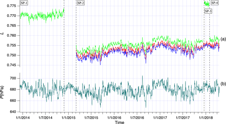
Figure 9. Time variations in daily data for the NM at the South Pole. (a) Uncorrected and unnormalized leader fraction L for all three counter tubes, indicating the start of each normalization period (SP-1 to SP-4) with significantly different firmware or software. (b) Atmospheric pressure as measured at the South Pole.
Download figure:
Standard image High-resolution imageTable 2. Time Periods of Neutron Time-delay Data Collection from the 3 × 1NM64 at the South Pole
| Normalization | Start Date | End Date | Cadence | Firmware Series | Software Versiona |
|---|---|---|---|---|---|
| Period | (Number of Tubes) | ||||
| SP-1 | 2013 Dec 9 | 2014 Nov 27 | Hourly | 600 (1) | ⋯ |
| SP-2a | 2015 Mar 3 | 2015 Mar 5 | Hourly | 800 (3) | 8.47 |
| SP-2b | 2015 Mar 6 | 2017 Dec 9 | Hourly | 800 (3) | 8.50–8.80 |
| SP-3 | 2017 Dec 18 | 2018 Jan 30 | Hourly | 600 (1), 800 (2) | 8.80 |
| SP-4 | 2018 Jan 31 | 2018 Apr 19 | Hourly | 800 (3) | 8.80 |
Note.
aOnly relevant for 800 series firmware.Download table as: ASCIITypeset image
Next, we aimed to calibrate L from the 600 and 800 series firmware. In period SP-3, starting on 2017 December 18 and ending on 2018 January 30, we installed 600 series firmware on NM tube 3, and the 800 series was still used on tubes 1 and 2. After calibration, starting 2018 January 31 (SP-4), we used 800 series firmware on all tubes. Our analysis ends on 2018 April 19.
Appendix C: Normalization of the Doi Inthanon Leader Fraction
The pressure- and water vapor–corrected L for each counter tube is different mainly due to its position and electronic dead time (Ruffolo et al. 2016). When we average L from all valid tubes for good statistics, this difference could lead to a change in the average value when the data from an individual tube are missing. Therefore, for the PSNM, we first normalized L from each counter tube to the average of L of a standard set of tubes, defined as the 10 counter tubes T2–T6 and T13–T17, based on the statistics of measured L ratios. This set was chosen to avoid the two end tubes, which have different energy responses and were swapped on 2014 December 7, and the six central tubes, which had different firmware versions from other tubes during calibration periods DI-6 and DI-8. These ratios were slightly dependent on the firmware, so we found the mean ratios for each firmware. To determine the mean ratios, for the 600 series firmware, we used the data of L only from period DI-1b (with hourly measurements) for better statistics; for the 700 series firmware, we used the data of L from DI-2; and for the 800 series firmware, we used L during DI-7 and DI-9. On 2014 December 7 (the start of DI-4b), we swapped the end tubes T1 and T18, and before that, 800 series firmware was used only for a short time with daily cadence during DI-4a, so we cannot accurately normalize T1 and T18, and data from these end tubes were not used for this time period.
We aim to normalize all leader fraction data to the standard set of 10 tubes using 800 series firmware with recent software versions on the newer computer, i.e., during time periods DI-6b, DI-7, and DI-9. For 800 series firmware, we found a systematic effect from histograms of the older software versions 8.34–8.47 used during DI-4, which provide a higher value of L than the newer software versions 8.50–8.124 as seen in Figure 8(a). There were apparently no other changes in L associated with changes in software. Therefore, we performed an experiment on 2018 March 20 to simultaneously collect time-delay histograms using software versions 8.47 (an older version) and 8.117 (a newer version). The mean ratio of L as calculated from these two software versions was used to normalize L from normalization period DI-4.
During part of DI-6a, starting on 2016 February 4, we operated two data acquisition computers to collect the time-delay histograms at the same time. Afterward, we used only the newer computer starting on 2016 May 18 (start of DI-6b). We found a difference in L for 800 series firmware, and we used the average ratio between L from the older computer and newer computer, found to be 0.99907 ± 0.000017, to normalize L from the older computer during DI-5 and DI-6a, for which we used newer software versions (8.50–8.82). This normalization was not applied to L from DI-4, when older software versions were used (8.34–8.47). These data are already normalized from the directly measured L ratio between older and newer software versions as described above, which leads to a continuous time series of L. If we were to perform an additional normalization for the change in the computer, as measured for newer software versions, the time series would become discontinuous. We conclude that the older software versions may be insensitive to the data acquisition computer.
We obtained consistent results, i.e., a reasonably continuous time series, when using the mean ratio of L from normalization period DI-8 to normalize L from 600 series firmware (during DI-1) or 700 series firmware (during DI-2 and DI-3) to 800 series firmware. It was also found that the ratio of L from 600 to 800 series firmware was different during the two calibration periods DI-6 and DI-8. This could be attributed to the higher level of solar modulation during DI-6 compared with DI-8, which was similar to that during DI-1 to DI-3. With the change in the cosmic-ray spectrum, it is possible that the different firmware series (which have different time-delay dead times) are affected differently; i.e., the ratio of L values from different firmware could be affected. For this reason, we consider it more appropriate to normalize DI-1 to DI-3 using the calibration from DI-8.
Finally, we obtain the time series of L as shown in Figure 4.
Appendix D: Normalization of the South Pole Leader Fraction
According to Figure 9, for the South Pole station, the leader fraction is different for different tubes. The physical reason is not clear, because each tube is in an individual insulated box, and all tubes have a similar dead time. In any case, after correction for pressure variations, we normalize the data from period SP-1 (using 600 series electronics only on tube 3) to periods SP-2 and SP-4 (using 800 series electronics on all three tubes), with data from the calibration period SP-3 (using 800 series on tubes 1 and 2 and 600 series on tube 3). Tubes 1 and 2 are the standard tubes for the purposes of normalization. After a normalization procedure similar to that described in the previous subsection, we obtain the time series of L as shown in Figure 5.
As noted earlier, the leader fraction from 2013 December to 2014 November (SP-1) has a much higher statistical uncertainty because time-delay histograms were only available for tube 3 using 600 series electronics, which collected time-delay data at 16 Hz, whereas at later times, the 800 series electronics allowed collection at the full rate of ∼100 Hz per tube for all three counter tubes. Furthermore, based on our experience at Doi Inthanon, we consider the normalization of SP-1 to be uncertain, because the normalization was based on the calibration period SP-3 (2017 December to 2018 January), when solar modulation conditions were very different. Therefore, in Figures 5 and 7, L data from SP-1 are plotted in blue to highlight their uncertain normalization relative to later data (in black).
Appendix E: Relation between the Doi Inthanon Leader Fraction and Spectral Index for a Model GCR Spectrum
In order to determine the relationship between the leader fraction L at Doi Inthanon and the spectral index for a GCR spectrum, we have performed Monte Carlo calculations and employed a simple model spectrum to determine L. Note that we do not recommend this as a realistic model of the spectrum. The motivation is explained in Section 4.2; here we report the details of the calculations.
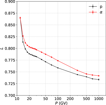
When analyzing time-delay histograms, we statistically determine the leader fraction L, i.e., the number of "leader" counts (that did not follow another count in the same counter tube associated with the same primary cosmic ray) divided by the total number of counts. Here we have used Monte Carlo simulation with the methods of Mangeard et al. (2016b), including geomagnetic effects, to calculate the yield function (count rate per GCR ion flux impinging on Earth's atmosphere) for the total counts (Yt,i) and leader counts (Yl,i), where i = p for primary protons and i = α for primary alpha particles (4He). Following standard practice in the field, because most cosmic-ray ions with atomic number Z ≥ 2 have Z/A ≈ 0.5 like 4He, they are accounted for by increasing the alpha flux by a factor F, which we vary between 1.4 and 1.6 to encompass the values used by Usoskin et al. (2011) and Mangeard et al. (2016b) following Caballero-Lopez & Moraal (2012), with a nominal value of 1.5. The yield functions are shown in Table 3. Figure 10 shows  (a weighted average over the 16 middle tubes) that would be expected for a specific primary cosmic-ray species i and rigidity P. Note that the upturn in L at P < 20 GV is associated with the geomagnetic cutoff at Doi Inthanon and does not appear if geomagnetic effects are not included.
Figure 10. Simulated leader fraction L for the 18NM64 at Doi Inthanon from Monte Carlo calculations for primary cosmic-ray protons (black) and alphas (red) as a function of primary rigidity P. Here L is a weighted average over the 16 middle counter tubes. The upturn for P < 20 GV is associated with the geomagnetic cutoff at Doi Inthanon.
Download figure:
Standard image High-resolution image
Table 3. Yield Functions for Total Counts (Yt,i) and Leader Counts (Yl,i) in Counts (particle cm−2 sr−1)−1 for i = p, α Summed over the 16 Middle Counter Tubes of the PSNM
| Rigidity (GV) | Yt,p | Yl,p | Yt,α | Yl,α |
|---|---|---|---|---|
| 10 | 0.00E+00 | 0.00E+00 | 0.00E+00 | 0.00E+00 |
| 12 | 7.19E+01 | 6.21E+01 | 1.71E+02 | 1.48E+02 |
| 14 | 3.33E+03 | 2.71E+03 | 6.99E+03 | 5.78E+03 |
| 16 | 1.10E+04 | 8.79E+03 | 2.35E+04 | 1.91E+04 |
| 18 | 1.95E+04 | 1.55E+04 | 4.19E+04 | 3.38E+04 |
| 20 | 2.72E+04 | 2.14E+04 | 5.88E+04 | 4.73E+04 |
| 22 | 3.33E+04 | 2.62E+04 | 7.29E+04 | 5.84E+04 |
| 24 | 3.86E+04 | 3.04E+04 | 8.44E+04 | 6.76E+04 |
| 26 | 4.26E+04 | 3.34E+04 | 9.45E+04 | 7.56E+04 |
| 28 | 4.63E+04 | 3.62E+04 | 1.04E+05 | 8.26E+04 |
| 30 | 4.96E+04 | 3.88E+04 | 1.11E+05 | 8.87E+04 |
| 40 | 6.36E+04 | 4.94E+04 | 1.44E+05 | 1.14E+05 |
| 50 | 7.61E+04 | 5.87E+04 | 1.68E+05 | 1.32E+05 |
| 70 | 9.91E+04 | 7.58E+04 | 2.12E+05 | 1.66E+05 |
| 100 | 1.30E+05 | 9.89E+04 | 2.79E+05 | 2.16E+05 |
| 300 | 3.03E+05 | 2.25E+05 | 6.60E+05 | 4.97E+05 |
| 500 | 4.59E+05 | 3.40E+05 | 1.00E+06 | 7.46E+05 |
| 700 | 6.36E+05 | 4.68E+05 | 1.30E+06 | 9.69E+05 |
| 1000 | 8.72E+05 | 6.40E+05 | 1.73E+06 | 1.28E+06 |
Download table as: ASCIITypeset image
There are two differences between the total yield functions presented here and those presented by Mangeard et al. (2016b). One concerns the electronic dead time, i.e., the time after a neutron event when another event cannot be recorded. While Mangeard et al. (2016b) used the count rate dead time (19–29 μs), here we use the dead time for time-delay histograms, which ranges from 72 to 83 μs for the 18 NM counter tubes at the PSNM when using 800 series firmware (to which the L data have been normalized; see Appendix C). Another difference is that here we present yield functions for the summed count rate of the 16 middle counter tubes (i.e., excluding end tubes 1 and 18), because our measurements of L have been normalized to the values for 10 middle tubes, and there is little difference in the spectral response for L among middle tubes.
Now we turn to the model GCR spectrum used to calculate the effect on L of the spectral index over ∼17–40 GV; some scientific justification for this simplified model was provided in Section 4.2. For protons and alphas, we use different continuous broken power-law rigidity spectra j(P) with a break at P = 40 GV, where  . Based on measurements in low Earth orbit by the AMS-02 instrument (Aguilar et al. 2015a, 2015b), we set the model spectrum as follows. The upper power-law indices are
  and
and  . The lower power-law index for protons,
  , is a free parameter, i.e., varying according to solar modulation; a nominal value is
  . Note that because of the geomagnetic cutoff at Doi Inthanon, and because the spectrum above 40 GV is held fixed (to model the lack of solar modulation at very high rigidity), the calculation is mainly sensitive to the model spectrum variation over ∼20 to 40 GV. Based on Figure 2(c) of Aguilar et al. (2015b) for that rigidity range, we use
  .
.
The relative normalization between p and α rigidity spectra is set at 40 GV. First, the pure α spectrum is normalized to 1, and then the p spectrum is normalized to 4.85 based on Figure 2(b) of Aguilar et al. (2015b). Then the α spectrum is renormalized to F (a free parameter) to account for all primary GCRs with Z ≥ 2.
Finally, the leader fraction is determined from
For the nominal values of F = 1.5 and  , we obtain L = 0.7819, which is higher than the measured values (see Figure 6) by about 0.008. For comparison, the Monte Carlo results of Mangeard et al. (2016a) for L as a function of cutoff rigidity were offset about 0.01 below the values of L measured by an NM latitude survey. Like that work, we will focus on relative changes in L. Increasing F by 0.1 caused an increase in L by 0.0002 and had a negligible effect on
  . For F between 1.4 and 1.6, and for
  near the nominal value, we find that
  . In other words, the full solar cycle variation in L observed at the PSNM, about 0.0008, corresponds to a change of ≈0.2 in the spectral index over ∼17–40 GV for this model spectrum.