


Abstract
Superflares, which are strong explosions on stars, have been well studied with the progress of spacetime-domain astronomy. In this work, we present the study of superflares on solar-type stars using Transiting Exoplanet Survey Satellite (TESS) data. Thirteen sectors of observations during the first year of the TESS mission covered the southern hemisphere of the sky, containing 25,734 solar-type stars. We verified 1216 superflares on 400 solar-type stars through automatic search and visual inspection with 2 minute cadence data. Our result suggests a higher superflare frequency distribution than the result from Kepler. This may be because the majority of TESS solar-type stars in our data set are rapidly rotating stars. The power-law index γ of the superflare frequency distribution ( ) is constrained to be γ = 2.16 ± 0.10, which is a little larger than that of solar flares but consistent with the results from Kepler. Because only seven superflares of Sun-like stars are detected, we cannot give a robust superflare occurrence frequency. Four stars were accompanied by unconfirmed hot planet candidates. Therefore, superflares may possibly be caused by stellar magnetic activities instead of planet–star interactions. We also find an extraordinary star, TIC43472154, which exhibits about 200 superflares per year. In addition, the correlation between the energy and duration of superflares (
 ) is analyzed. We derive the power-law index to be β = 0.42 ± 0.01, which is a little larger than β = 1/3 from the prediction according to magnetic reconnection theory.
Export citation and abstract BibTeX RIS
1. Introduction
Solar activities are closely connected with the lives of human beings. For example, solar winds can affect space weather, and trigger geomagnetic storms on Earth. Solar activities thus have large impacts on many fields, e.g., spacecraft electronics, commercial aviation, and radio communication (Choi et al. 2011). The Carrington event (Carrington 1859), which generated a very large solar flare with a total energy up to 1032 erg, caused widespread disruption of telegraph systems and is considered to be one of the most severe solar storms to date. An indication of this event is also found in polar ice (Shea et al. 2006). However, the reliability of nitrate in ice records as a proxy for solar flares is strongly debated (Melott et al. 2016; Mekhaldi et al. 2017).
Solar flares are also studied by indirect methods, such as rapid increases of 14C in tree rings. Four such events have been found (Miyake et al. 2012, 2013; Park et al. 2017; Wang et al. 2017). Based on the fact that quasi-simultaneous peaks of 10Be and 36Cl are found to be associated with peaks of 14C, solar superflares are considered as their physical origin (Mekhaldi et al. 2015; Miyake et al. 2019). However, the peaks of 10Be and 36Cl are adjusted to fit the 14C peaks (Mekhaldi et al. 2015). So, if the peaks really are simultaneous, a solar origin is the most probable (Mekhaldi et al. 2015; Miyake et al. 2019). If these peaks are not correlated, other models may be possible (Neuhäuser & Hambaryan 2014, 2015; Wang et al. 2019).
Superflares are much stronger explosions than typical solar flares, with total energies varying from 1033–1038 erg and durations of longer than an hour. The energy of a superflare is so high that it can directly harm nearby living creatures. This has therefore attracted people's interest as to whether our Sun can generate superflares, just like the nine main sequence F8–G8 stars near our solar system (Schaefer et al. 2000). Previous studies have revealed a power-law relation between flare energy and frequency  (Dennis 1985), which can be explained by self-organized criticality happening in a nonlinear energy dissipation system (e.g., Bak et al. 1987; Lu & Hamilton 1991; Aschwanden 2011; Wang & Dai 2013). For hard X-ray solar flares, γ was estimated to be 1.53 ± 0.02 by Crosby et al. (1993). For nanoflares and microflares, γ is 1.79 ± 0.08 (Aschwanden et al. 2000) and 1.74 (Shimizu 1995), respectively. With the help of the Kepler space telescope, Maehara et al. (2012) detected 101 superflares on 24 slowly rotating solar-type stars and derived γ = 2.0 ± 0.2, which is very similar to that of the distribution of solar flares. This therefore suggests there is a possibility for superflares to occur on the Sun, but with a comparatively lower frequency than rapidly rotating G-type stars.
There have been many observational and theoretical studies since the discovery of superflares on G-type stars with Kepler data. Shibayama et al. (2013) and Notsu et al. (2013) studied the connection between superflares and starspots by using more samples, and concluded that the energy of superflares is related to the starspot coverage, which is similar to the relation between solar flares and sunspots. Note that although the samples from Shibayama et al. (2013) were mistakenly mixed with some stars which are not in the main sequence, their conclusions are not changed (Notsu et al. 2019). Large starspots can be generated by a solar dynamo mechanism (Shibata et al. 2013) and may store energy for superflares. Superflares, therefore, may have the same origin as solar flares. Because the Kepler input catalog may not give an accurate estimation of the properties of solar-type stars, ground-based follow-up observations were also dedicated to the research, which has constrained stellar periodicity and spectrum information (Notsu et al. 2015a, 2015b). Maehara et al. (2015) supported the comparability by extending the flares to lower energies using the 1 minute short-cadence data from Kepler. Karoff et al. (2016) also provided support by analyzing the chromospheric activities of 5648 Sun-like stars and 48 superflare stars in the field of view of both Kepler and the Large Sky Area Multi-Object Fibre Spectroscopic Telescope (LAMOST).
On the other hand, there are different explanations for superflares. Rubenstein & Schaefer (2000) argued that a hot Jupiter companion can cause superflares on a solar-type star. Numerical simulations by Ip et al. (2004) also presented the importance of the effect of planet–star magnetic interactions on stellar activities. In addition, He et al. (2015) argued that the rotational modulation may be caused by faculae instead of starspots. It is also possible that flares and the magnetic features that dominate rotational modulation may possibly have different source regions (He et al. 2018).
In this paper, we aim to detect superflares on solar-type stars using Transiting Exoplanet Survey Satellite (TESS) data. The primary goal of TESS is to find planets around bright nearby stars to enable further ground-based follow-up observations (Ricker et al. 2015). TESS has three advantages for studying stellar flares. First, the stars observed by TESS are bright enough to achieve a high signal-to-noise ratio. Second, the 2 minute cadence allows the study of more detailed flare properties, such as duration and energy. Besides, to obtain more credible stellar parameters, the TESS input catalog (TIC) has imported data from other space and ground-based projects, such as Gaia-DR1 and 2 and LAMOST-DR1 and DR3.
This paper is constructed as follows. In Section 2, we describe the methods to select solar-type stars and superflare candidates from the TESS data. Stellar periodicity and flare energy are also derived. The main results are described and discussed in Section 3, including the occurrence frequency of superflares, active flare stars, systems with exoplanets, and the correlation between the duration and energy of superflares. Finally, we summarize our findings in Section 4.
2. Data and Methods
2.1. Selection of Solar-type Stars
TESS was launched on 2018 April 18, and carries four identical cameras. During its first year of observations, TESS has scanned the southern hemisphere of the sky and obtained data products for 13 segments (sector 1–sector 13). Each segment covers about 27 days. In this work, we adopt the presearch data conditioned (PDC) light curves to avoid the instrumental systematics.
First, the selection criteria of solar-type stars and Sun-like stars should be clarified. Solar-type stars are selected according to following criteria: (1) the surface effective temperature satisfies  and (2) the surface gravity in log scale is log g > 4.0 (Schaefer et al. 2000; Maehara et al. 2012). Those solar-type stars with
  and stellar periodicity >10 days are considered as Sun-like stars. In total, 26,034 targets meet the requirements based on the latest TIC v8 (Stassun et al. 2019), which is expected to be the last version of the TIC. Then, we examine these solar-type stars with the Hipparcos-2 catalog (van Leeuwen 2007) to exclude some confirmed binary stars. In total, 145 stars are excluded from the data set.
In contrast to Kepler, of which the pixel scale is about 4'', TESS has a larger pixel scale of 21''. 90% of the energy is ensquared by 4 × 4 pixels, in other words, it is encircled by a radius of 42'' (Ricker et al. 2015). Therefore, it is possible that in one pixel from TESS, the primary object is contaminated by other stars. Therefore, we use Gaia-DR2 (Gaia Collaboration et al. 2018) to search for stars within a 42'' radius near the primary solar-type star. Within a 21'' radius, we find 155 stars containing other brighter stars, which are excluded from the data set. The reasons for this are: (1) flux from these brighter stars may significantly affect the light curves of the main target; and (2) in just one pixel scale (21''), we cannot separate these brighter stars apart from main targets. Next, 2849 solar-type stars, of which the nearby stars show a surface effective temperature within 3000 K–4000 K, are flagged as possessing M dwarf candidates. The reason why they are not excluded from the data set is shown in Appendix A.
2.2. Selection of Superflares
The PDC light curves of the solar-type stars are used to search for superflares. There are several selection methods in the literature. For example, clean light curves with only flare candidates can be acquired by fitting the quiescent variability (e.g., Walkowicz et al. 2011; Wu et al. 2015; Yang & Liu 2019). In addition, flare candidates can also be obtained by calculating the distribution of brightness changes between consecutive data points (e.g., Maehara et al. 2012; Shibayama et al. 2013; Maehara et al. 2015). In this paper, we choose the latter method to detect superflares. According to Maehara et al. (2015), brightness changes between two pairs of consecutive points ΔF2 are defined as:

where Fi and ti represent the flux and the time of the ith data point, n is an integer number, and s = ±1. s = 1 when both  and
and  , otherwise s = −1. ΔF2 during a superflare event will become much larger than the quiescent situation. We set n = 2 to detect flare candidates with rise times larger than 4 minutes (Maehara et al. 2015). Besides, we also set n = 5 and obtained another group of ΔF2 in case of missing flares with longer rise times. A data point is recognized as a flare candidate when its ΔF2 is at least three times larger than the value at the top 1% of the ΔF2 distribution. We then located the peak data point for each flare candidate. To obtain a complete flare event, we use the data from 0.05 to 0.01 days before the peak and from 0.05 to 0.10 days after the peak in the case of n = 2, and use the data from 0.15 to 0.03 days before the peak and from 0.15 to 0.25 days after the peak in the case of n = 5. A quadratic function, Fq(t), is adopted to remove the long-term stellar variability. The start time and end time of each flare candidate are the first and last point when F(t) − Fq(t) is three times larger than the photometric error. We only reserve a flare candidate when (1) there are at least three consecutive points during the spike event, and (2) the decay time is longer than the rise time.
Then, we check each flare candidate by using pixel-level data to exclude false positives such as eclipses, random flux jumps, and cosmic rays. First, we remove the candidates occurring simultaneously on different stars. Second, the pixel-level light curves during the flare event should match the optimal aperture given by TESS. Third, visual inspection is applied to ensure the flare-like shape and obvious flux increases in pixel-level light curves as suggested by Wu et al. (2015). We present the example of a true flare event in Figure 1. The light curve of TIC121011020 in sector 4 perfectly shows a standard case of a flare-shaped curve, with rapid rise and slow decay. Figure 2 shows a case with pixel-level fluctuations under the noise level. We exclude it from superflares since it is more likely to be a very weak flare or just noise. After excluding all the false positives, we finally find 1216 superflares occurring on 400 solar-type stars.

Figure 1. An example of a true flare event. The upper panel gives a flare light curve of TIC121011020. The black solid line stands for normalized flux F(t). The flux fitted by the quadratic function ( ) is shown as a red solid line. The red, yellow, and blue points represent the beginning, peak, and end times of the flare, respectively. The light curve in this panel shows a standard flare shape with a rapid rise and slow decay. The lower-left panel shows pixel-level data at the peak time. The blue frames encircle TESS pipeline aperture masks. Those pixels are masked with a deeper blue where the flux is greater than the others. In the lower-right panel, we present the light curves of each target pixel, which corresponds to every single block in the lower-left panel. The blue light curves stand for TESS pipeline aperture masks. We may conclude from this panel that the flare-shape light curves are distributed as a point-spread function (PSF).
Download figure:
Standard image High-resolution image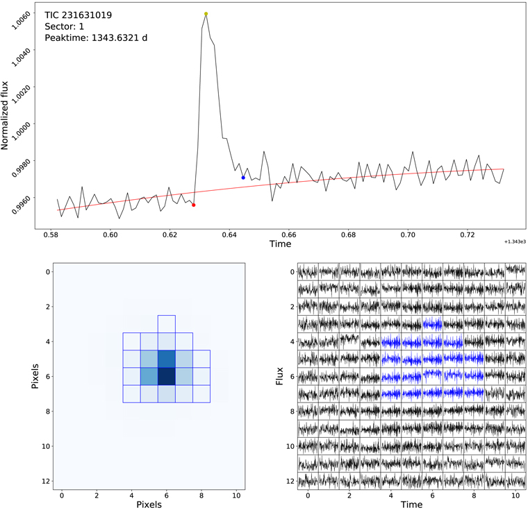
Figure 2. Same as Figure 1, but for a false event or a very weak flare, which is excluded from the flare candidates. In the lower-right panel, unlike what we perceive from Figure 1, it may not show light curves distributed as a PSF. But the noise level flux has been flooded in all pixels.
Download figure:
Standard image High-resolution image2.3. Periodicity Estimation
The periodicity of the solar-type stars are estimated through the Lomb–Scargle method (Lomb 1976; Scargle 1982), which is suitable for unevenly sampled data (VanderPlas 2018). We set the false alarm probability to 10−4 to search the stellar period (e.g., Cui et al. 2019).
Figure 3 presents the period distributions of the solar-type stars, superflares and flare stars. Note that we may miss some slowly rotating solar-type stars with P > 10 days because of the limited observing span. Most of the TESS targets were observed only in one sector, i.e., about 27 days, as shown in Figure 4. Therefore, periods longer than ∼14 days are not reliable for these targets. In total, we obtain stellar periods for 3827 slowly rotating (P > 10 days) solar-type stars and 22,207 fast rotating (P < 10 days) solar-type stars.

Figure 3. Periodic distribution of solar-type stars (solid line), superflares (dotted line), and flare stars (dashed line). Table 3 lists the corresponding values of each subset.
Download figure:
Standard image High-resolution image
Figure 4. Distribution of solar-type stars (solid line), superflares (dotted line), and flare stars (dashed line) in each Set-n subset. The definition of Set-n can be found in Section 3.1. Table 4 lists the corresponding values of each subset.
Download figure:
Standard image High-resolution image2.4. Energy of Superflares
Following the method of Wu et al. (2015), the stellar luminosity can be estimated with the Stefan–Boltzmann law

where R* and T* are the stellar radius and effective temperature given by TIC v8, and σsb is the Stefan–Boltzmann constant. The flare energy thus can be calculated by integrating the fluxes within the flare event

where  is the normalized flux above the fitted quadratic function (see Section 2.2)

3. Results
In Table 1, we list all parameters of 400 flare stars. Table 2 gives the parameters of 1216 superflares. Table 3 present the period distributions of the solar-type stars, superflares, and flare stars.
Table 1. Flare Stars
| TESS ID | Teffa | log gb | Radiusc | Periodd | Flarese | Set-nf | f*g | Flagh |
|---|---|---|---|---|---|---|---|---|
| (K) | (R⊙) | (days) | (yr−1) | |||||
| 737327 | 5872 | 4.20 | 1.35 | 1.62 | 1 | 1 | 14.57 | GM |
| 1258935 | 5739 | 4.48 | 0.97 | 4.93 | 1 | 1 | 19.37 | |
| 6526912 | 5541 | 4.24 | 1.25 | 2.29 | 1 | 1 | 14.39 | |
| 7491381 | 5692 | 4.47 | 0.96 | 2.21 | 4 | 3 | 21.37 | |
| 7586485 | 5801 | 4.36 | 1.11 | 1.76 | 6 | 2 | 46.11 | |
| 11046349 | 5409 | 4.31 | 1.12 | 3.33 | 2 | 1 | 29.48 | GM |
| 12359032 | 5471 | 4.51 | 0.90 | 2.32 | 2 | 1 | 27.98 | |
| 12393800 | 5571 | 4.19 | 1.31 | 1.03 | 1 | 1 | 13.99 | |
| 13955147 | 5701 | 4.44 | 1.01 | 2.22 | 1 | 2 | 7.69 | |
| 15444490 | 5598 | 4.09 | 1.49 | 1.98 | 2 | 2 | 15.85 |
Notes.
aEffective surface temperature in K. bSurface gravity of star in log scale. cStellar radii in units of solar radius R⊙. dStellar periods in days. eNumber of flares of each star (same as N*flares of Equation (9)). fNumber of Set-n which defined in Section 3.1. gFlare frequency deduced by Equation (9). hFlags of flare stars, where GM means the star may possess M dwarf candidates nearby (42'' from the main target). GB indicates that there are stars that are brighter than the main stars, and 21–42'' from the main targets. (A portion of data is shown here. The full data is available in machine-readable form online.)Only a portion of this table is shown here to demonstrate its form and content. A machine-readable version of the full table is available.
Download table as: DataTypeset image
Table 2. Superflares
| TESS ID | Peak Datea | Peak Fluxb | Energyc | Durationd |
|---|---|---|---|---|
| (erg s−1) | (erg) | (s) | ||
| 737327 | 1460.1798 | 5.02E+31 | 5.58E+34 | 1919.98 |
| 1258935 | 1517.6755 | 4.71E+31 | 3.97E+34 | 1560.03 |
| 6526912 | 1673.3840 | 3.78E+32 | 9.46E+35 | 5759.94 |
| 7491381 | 1469.0019 | 1.10E+32 | 7.96E+34 | 1559.99 |
| 7491381 | 1470.5130 | 4.08E+31 | 9.09E+34 | 3359.98 |
| 7491381 | 1486.3100 | 3.71E+31 | 2.32E+34 | 959.98 |
| 7491381 | 1489.2516 | 6.92E+31 | 2.12E+35 | 6959.85 |
| 7586485 | 1411.2694 | 5.53E+31 | 6.91E+34 | 2640.06 |
| 7586485 | 1428.4168 | 3.61E+31 | 4.75E+34 | 2520.01 |
| 7586485 | 1440.9098 | 2.07E+31 | 1.39E+34 | 959.99 |
| 7586485 | 1442.7237 | 9.31E+31 | 5.07E+34 | 1559.99 |
| 7586485 | 1447.3084 | 3.15E+31 | 4.37E+34 | 2279.97 |
| 7586485 | 1457.0429 | 3.82E+31 | 8.09E+34 | 3599.92 |
Notes.
aThe corresponding date of the superflares' peak. bFlux of peak calculated by L* Fflare(t), when t equals to the peak time. L* and Fflare(t) are defined in Equations (2) and (4). cEnergy of the superflares. dDuration of the superflares in seconds. (A portion of data is shown here. The full data is available in machine-readable form online.)Only a portion of this table is shown here to demonstrate its form and content. A machine-readable version of the full table is available.
Download table as: DataTypeset image
3.1. Occurrence Frequency Distribution
The observation mode of TESS, unlike Kepler, causes various observing spans for different targets. It is not suitable for calculating the occurrence frequency of superflares directly using the unequal observing spans. We therefore improve the method suggested by Maehara et al. (2012). First of all, we subdivided all the solar-type stars into different sets based on how many sectors the star was observed in. For example, Set-1 means that the stars were observed in only one sector. Similarly, Set-13 covers the stars observed in all 13 sectors. The count of the solar-type stars in each Set-n can be found in Figure 4 and Table 4.
Table 3. Numbers of Solar-type Stars, Superflares, and Flare Stars of Each Periodic Bin
| log P | Solar-type Stars | Superflares | Flare Stars |
|---|---|---|---|
| −1.00 | 585 | 2 | 2 |
| −0.81 | 606 | 8 | 1 |
| −0.62 | 408 | 22 | 9 |
| −0.43 | 372 | 46 | 13 |
| −0.24 | 390 | 95 | 28 |
| −0.05 | 543 | 136 | 41 |
| 0.14 | 919 | 295 | 80 |
| 0.33 | 2900 | 317 | 90 |
| 0.52 | 4486 | 217 | 82 |
| 0.71 | 7410 | 50 | 35 |
| 0.90 | 5728 | 22 | 16 |
| 1.10 | 1151 | 2 | 2 |
| 1.29 | 113 | 4 | 1 |
| 1.48 | 111 | 0 | 0 |
| 1.67 | 7 | 0 | 0 |
| 1.86 | 3 | 0 | 0 |
| 2.05 | 2 | 0 | 0 |
Note. log P represents stellar periodicity in the log scale.
Download table as: ASCIITypeset image
Table 4. Numbers of Solar-type Stars, Superflares, and Flare Stars of Each Set-n
| Set-n |

|

|
Total | ||||||||||||
|---|---|---|---|---|---|---|---|---|---|---|---|---|---|---|---|
| P < 10 days | P > 10 days | P < 10 days | P > 10 days | ||||||||||||
| Nstar | Nflare | Nfstar | Nstar | Nflare | Nfstar | Nstar | Nflare | Nfstar | Nstar | Nflare | Nfstar | Nstar | Nflare | Nfstar | |
| 1 | 7023 | 249 | 128 | 1204 | 0 | 0 | 8798 | 113 | 67 | 1018 | 5 | 2 | 18043 | 367 | 197 |
| 2 | 1465 | 233 | 67 | 406 | 0 | 0 | 1894 | 113 | 36 | 335 | 0 | 0 | 4100 | 346 | 103 |
| 3 | 326 | 34 | 14 | 88 | 0 | 0 | 471 | 39 | 14 | 80 | 1 | 1 | 965 | 74 | 29 |
| 4 | 92 | 16 | 3 | 24 | 0 | 0 | 123 | 11 | 3 | 14 | 0 | 0 | 253 | 27 | 6 |
| 5 | 73 | 0 | 0 | 19 | 0 | 0 | 109 | 0 | 0 | 15 | 0 | 0 | 216 | 0 | 0 |
| 6 | 54 | 18 | 2 | 14 | 0 | 0 | 68 | 18 | 3 | 21 | 0 | 0 | 157 | 36 | 5 |
| 7 | 39 | 65 | 5 | 16 | 0 | 0 | 63 | 3 | 1 | 13 | 0 | 0 | 131 | 68 | 6 |
| 8 | 37 | 1 | 1 | 15 | 0 | 0 | 48 | 5 | 2 | 15 | 0 | 0 | 115 | 6 | 3 |
| 9 | 80 | 31 | 5 | 29 | 0 | 0 | 90 | 1 | 1 | 25 | 0 | 0 | 224 | 32 | 6 |
| 10 | 62 | 25 | 2 | 35 | 0 | 0 | 73 | 3 | 2 | 28 | 0 | 0 | 198 | 28 | 4 |
| 11 | 91 | 20 | 6 | 44 | 4 | 1 | 115 | 10 | 3 | 35 | 0 | 0 | 285 | 34 | 10 |
| 12 | 182 | 29 | 5 | 77 | 1 | 1 | 213 | 23 | 8 | 59 | 1 | 1 | 531 | 54 | 15 |
| 13 | 173 | 38 | 5 | 76 | 0 | 0 | 193 | 106 | 11 | 74 | 0 | 0 | 516 | 144 | 16 |
| Total | 9697 | 759 | 243 | 2047 | 5 | 2 | 12258 | 445 | 151 | 1732 | 7 | 4 | 25734 | 1216 | 400 |
Note. The definition of Set-n is in Section 3.1. Basically, according to the stellar surface temperature and rotation period, we classify solar-type stars into four categories for each Set-n. Nstar, Nflare, and Nfstar represent the numbers of solar-type stars, flares, and flare stars, respectively. The total numbers are also listed in the last three columns and the last row.
Download table as: ASCIITypeset image
For each Set-n, the superflare frequency distribution as a function of flare energy is defined as

where Nflares and Nstars are the numbers of superflares and solar-type stars in Set-n. ΔEflare represents the bin width of flare energy. τn can be calculated as

As the observing time is affected by satellite orbit, TESS may not fully and effectively observe for 27 days in each sector. Here, we calculated the mean value of continuous observation length of each sector, which is 23.4 days. The final occurrence frequency of superflares for all the solar-type stars can be calculated as

Figure 5(a) illustrates the distribution of flare peak amplitudes, i.e., the peak flux of Fflare(t) in Equation (4). Panel (b) presents the frequency distributions as a function of flare energy for all the solar-type stars (solid line), and slowly (dashed line) or rapidly (dotted line) rotating solar-type stars. After comparing the dotted and dashed lines, it is evident that rapidly rotating stars are much more active than slowly rotating stars. According to the relation between stellar periodicity and age (Skumanich 1972; Barnes 2003), this result therefore indicates that younger solar-type stars generate superflares more frequently.

Figure 5. (a) Frequency distribution of the normalized peak flux  at time tpeak. All 1216 superflares are included. (b) Frequency distribution of flare energy. The solid line represents all 1216 solar-type stars (with
  and log g > 4.0), and the dashed line expresses 12 superflares of slowly rotating solar-type stars (with a period P > 10 days). Two straight lines show the best-fit power-law distribution of
  . The solid line gives
  , and the dashed line gives
  . The dotted line stands for 1204 flares on rapidly rotating stars, of which frequency distributions almost overlap with the solid line. (c) The same frequency distribution as in (b) but for different effective surface temperatures. The solid and dashed lines represent data sets of
  and
and  respectively. (d) The solid line indicates the same frequency distribution as the solid line in (b). In contrast with the result of Kepler short-cadence data, we imported the result from Figure 3(b) of Maehara et al. (2015) as the dashed line. The dotted line indicates the frequency distribution of Sun-like stars with an effective temperature
  and period P > 10 days. However, only seven flares satisfy the two criteria. In all panels, the error bars are given by the square root of the flare numbers in each bin.
Download figure:
Standard image High-resolution imageA power-law model is used to fit the frequency distributions

The power-law index γ is fitted by using the same linear regression method as in Tu & Wang (2018). For all solar-type stars, γ is 2.16 ± 0.10, which is consistent with γ ∼ 2.2 from Shibayama et al. (2013) within a 1σ interval, but higher than γ ∼ 1.5 from Maehara et al. (2015). From Figure 5(c), it is obvious that hotter stars (with 5600 K ≤ Teff < 6000 K) have a lower frequency than cooler stars (with  ). The above results are basically similar to those found from Kepler data (Maehara et al. 2012; Shibayama et al. 2013; Maehara et al. 2015).
Figure 5(d) compares the flare frequency derived in this work and by Maehara et al. (2015), which used the 1 minute short-cadence data of Kepler and therefore detected more flares in the low-energy region (<2 × 1034 erg). In the high-energy region (>2 × 1034 erg), our superflare frequencies are higher than theirs. We speculate that this result is caused by the higher proportion of young stars in our data set, as we have discussed above (panel (b)). Since young stars rotate more rapidly and are more active, they are more likely to generate superflares. In total, 25,734 solar-type stars are selected, among which 21,955 stars have periods of less than 10 days. The proportion of young stars is 85% in our work, compared to 32% in the work by Maehara et al. (2015). One may refer to Appendix B for more discussions about the potential changes caused by the number fraction of rapidly and slowly rotating stars.
The superflare frequency of Sun-like stars (dotted line) is also presented in Figure 5(d). For Sun-like stars (with  and P > 10 days), we obtain a higher frequency of superflares (>1035 erg) than that from Kepler (Maehara et al. 2012; Shibayama et al. 2013; Maehara et al. 2015). However, there are only seven such events, which are insufficient to robustly make a statistical conclusion. We look forward to more observations from TESS to extend the sample of Sun-like stars.
3.2. Stellar Period versus Superflare Energy
An apparent negative correlation between flare frequency and stellar period has been found (Maehara et al. 2012; Notsu et al. 2013; Maehara et al. 2015). In Figure 6(b), in the range of the stellar period over a few days, it is clear that the flare frequency decreases with an increase of the rotation period. A similar result is found by Notsu et al. (2013) and Notsu et al. (2019). Moreover, stellar age has a positive correlation with the stellar period (Skumanich 1972; Barnes 2003). This result indicates that rapidly rotating stars, or young stars, are more likely to generate superflares.

Figure 6. (a) Scatter plot of superflare energy vs. stellar period. Black pluses denote every single superflare. (b) Flare frequency of each period bin; the error bars are given by the square root of flare numbers in each bin. (c), (d) Same as panel (a), but for superflares with different effective temperatures  (red squares) and
  (blue circles), respectively.
Download figure:
Standard image High-resolution imageNotsu et al. (2019) found that the upper limit of flare energy in each period bin has a continuous decreasing trend with the rotation period. From Figure 6(a), compared with the previous result (Figure 12(b) of Notsu et al. 2019), this trend is not obvious for the whole range of periods. However, superflares within the period range over a few days (the tail part) clearly show the decreasing trend. We separate superflares into two parts according to their surface effective temperatures, which are shown in Figures 6(c) and (d) respectively. Superflares with a temperature 5600 K ≤ Teff < 6000 K perhaps show a slightly more clear decreasing trend for the whole period range, compared with panel (a). A similar decreasing trend can also be found in these two panels with period range over a few days (the tail part). As period is the key factor, we look forward to other methods precisely determining the periods of these solar-type stars (Appendix B). Meanwhile, slow-rotation stars (P ∼ 25 days) need to be searched for specially, in order to statistically and strongly confirm this trend.
3.3. Active Flare Stars
Given that solar-type stars are grouped in different Set-n because of unequal observing spans, the flare frequency for an individual star is described by

where τ* is the continuous observation length of each flare star, and N*flares denotes the number of flares from an individual star.
Tables 5 and 6 list the top 20 stars sorted by flare frequency f* and the number of flares N*flares, respectively. TIC43472154 is the most active star with an impressive flare frequency. If it is not coincidentally observed at an extraordinary active period, TIC43472154 can generate 233.17 flares per year. Besides, this star is not accompanied by any fainter stars or M dwarfs, according to the cross-match results from Gaia and Hipparcos data. This occurrence rate is much higher than that of KIC10422252, which is 41.6 flares per year (Shibayama et al. 2013). Figure 7 plots the light curve of TIC43472154. Superflares are marked with downward arrows.
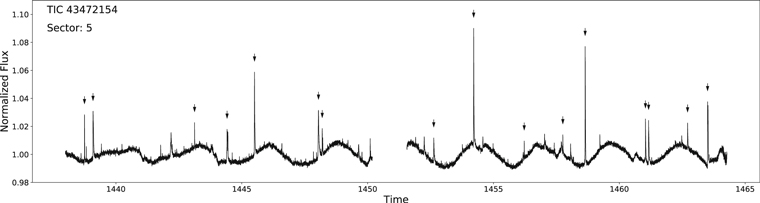
Figure 7. Light curve of TIC43472154. Small arrows mark those superflares selected from automatic software, and checked through a pixel-level pattern.
Download figure:
Standard image High-resolution imageTable 5. Stellar Properties of Flare Stars Sorted by Star Activity f*
| TESS ID | Teff a | log gb | Radius c | Period d | Flares e | Set-nf | f* g |
|---|---|---|---|---|---|---|---|
| (K) | (R⊙) | (days) | (yr−1) | ||||
| 43472154 | 5316 | 4.49 | 0.90 | 2.80 | 16 | 1 | 233.17 |
| 92845906 | 5634 | 4.17 | 1.37 | 2.07 | 22 | 2 | 175.12 |
| 53417036 | 5555 | 4.44 | 0.98 | 1.53 | 8 | 1 | 140.26 |
| 20096356 | 5458 | 4.46 | 0.95 | 0.79 | 16 | 2 | 127.34 |
| 175491080 | 5321 | 4.52 | 0.88 | 3.98 | 14 | 2 | 122.71 |
| 206592394 | 5597 | 4.54 | 0.88 | 3.43 | 8 | 1 | 111.91 |
| 38402758 | 5472 | 4.42 | 1.00 | 1.08 | 6 | 1 | 97.62 |
| 127311608 | 5515 | 4.23 | 1.25 | 0.96 | 5 | 1 | 93.24 |
| 382575967 | 5567 | 4.42 | 1.01 | 2.19 | 40 | 7 | 91.36 |
| 284789252 | 5789 | 4.41 | 1.05 | 0.87 | 6 | 1 | 88.45 |
| 92347098 | 5234 | 4.48 | 0.90 | 3.93 | 5 | 1 | 81.34 |
| 152346470 | 5844 | 4.14 | 1.44 | 1.97 | 5 | 1 | 81.08 |
| 78055898 | 5495 | 4.30 | 1.14 | 4.07 | 10 | 2 | 79.59 |
| 257644579 | 5916 | 4.38 | 1.11 | 1.51 | 10 | 2 | 76.86 |
| 364588501 | 5605 | 4.26 | 1.22 | 2.28 | 63 | 13 | 75.35 |
| 272456799 | 5874 | 4.14 | 1.46 | 2.18 | 4 | 1 | 74.60 |
| 21540586 | 5417 | 4.27 | 1.18 | 1.35 | 9 | 2 | 71.63 |
| 93277807 | 5706 | 4.17 | 1.37 | 3.89 | 4 | 1 | 70.15 |
| 32874669 | 5147 | 4.53 | 0.84 | 4.73 | 4 | 1 | 70.15 |
| 302116397 | 5531 | 4.39 | 1.05 | 0.95 | 5 | 1 | 67.93 |
Note. Top 20 flare stars sorted by flare frequency (f*). The headers of this table are the same as in Table 1.
Download table as: ASCIITypeset image
Table 6. Stellar Properties of Flare Stars Sorted by Number of Flares
| TESS ID | Teff a | log gb | Radius c | Period d | Flares e | Set-nf | f* g |
|---|---|---|---|---|---|---|---|
| (K) | (R⊙) | (days) | (yr−1) | ||||
| 364588501 | 5605 | 4.26 | 1.22 | 2.28 | 63 | 13 | 75.35 |
| 382575967 | 5567 | 4.42 | 1.01 | 2.19 | 40 | 7 | 91.36 |
| 149539114 | 5367 | 4.36 | 1.05 | 0.43 | 22 | 10 | 36.05 |
| 92845906 | 5634 | 4.17 | 1.37 | 2.07 | 22 | 2 | 175.12 |
| 260162387 | 5855 | 4.20 | 1.35 | 1.98 | 18 | 13 | 21.63 |
| 167163906 | 5465 | 4.55 | 0.86 | 0.76 | 18 | 12 | 23.44 |
| 279572957 | 5570 | 4.34 | 1.11 | 1.81 | 16 | 9 | 27.86 |
| 43472154 | 5316 | 4.49 | 0.90 | 2.80 | 16 | 1 | 233.17 |
| 20096356 | 5458 | 4.46 | 0.95 | 0.79 | 16 | 2 | 127.34 |
| 167574282 | 5291 | 4.53 | 0.86 | 1.70 | 14 | 13 | 16.73 |
| 175491080 | 5321 | 4.52 | 0.88 | 3.98 | 14 | 2 | 122.71 |
| 339668420 | 5395 | 4.47 | 0.93 | 4.84 | 12 | 6 | 32.34 |
| 219389540 | 5744 | 4.44 | 1.02 | 1.55 | 11 | 6 | 29.32 |
| 257644579 | 5916 | 4.38 | 1.11 | 1.51 | 10 | 2 | 76.86 |
| 78055898 | 5495 | 4.30 | 1.14 | 4.07 | 10 | 2 | 79.59 |
| 38827910 | 5304 | 4.53 | 0.86 | 3.66 | 10 | 11 | 14.14 |
| 348898049 | 5226 | 4.71 | 0.69 | 1.00 | 9 | 13 | 10.76 |
| 219212899 | 5217 | 4.55 | 0.83 | 4.06 | 9 | 7 | 20.53 |
| 21540586 | 5417 | 4.27 | 1.18 | 1.35 | 9 | 2 | 71.63 |
| 260268898 | 5186 | 4.58 | 0.80 | 2.25 | 8 | 9 | 13.97 |
Note. Top 20 flare stars sorted by the number of flares on the corresponding star. The headers of this table are the same as in Table 5.
Download table as: ASCIITypeset image
Another target, TIC364588501, was observed by all sectors of TESS and exhibits the largest number of flares (63). Additionally, like TIC43472154, this star is also a single star, according to the cross-match results from Gaia and Hipparcos data. TIC364588501 became more active than usual in the last 15 days of sector 5, and generated 15 superflares (Figure 8).

Figure 8. Same as Figure 7, but for TIC364588501.
Download figure:
Standard image High-resolution imageThe most energetic superflare comes from TIC93277807, releasing 1.77 × 1037 erg in around 1.5 hr. This value consists with the inference that energy releasing through a stellar flare is saturated at ∼2 × 1037 erg (Wu et al. 2015).
3.4. Planets of Flare Stars
Hot Jupiters are considered as one of the essential factors that can produce superflares on host stars (e.g., Rubenstein & Schaefer 2000; Ip et al. 2004). According to these studies, it is not possible for the Sun to generate superflares. However, a lot of statistical works based on Kepler data did not detect hot Jupiters around flare stars (Maehara et al. 2012; Shibayama et al. 2013; Maehara et al. 2015).
We made a cross-check between our 400 flare stars with the Exoplanet Follow-up Observing Program for TESS (ExoFOP–TESS3 ). Cross-matching results are listed in Table 7. There are four stars (TIC25078924, 44797824, 257605131, and 373844472) that have planet candidates. These four stars are unlikely to affect our statistical results. We thus did not exclude them in the analysis. Besides, there is only one star (TIC410214986) that possesses a confirmed hot planet (Newton et al. 2019). This is an interesting planet, and we list its parameters in Table 7, even if its hosting star (TIC410214986) is flagged as a binary system from the Hipparcos-2 catalog.
Table 7. Properties of Flare Stars Hosting Planets
| Host Star | Planet ID | Perioda | Radiusb | Equilibrium Temp.c | Informationd |
|---|---|---|---|---|---|
| TESS ID | (Days) | (R⊕) | (K) | ||
| 25078924 | TIC25078924.01 | 0.9097 | 14.43 | ⋯ | Community TESS objects of interest |
| 25078924 | TIC25078924.02 | 0.9035 | 28.70 | ⋯ | Community TESS objects of interest |
| 44797824 | TOI865.03 | 0.7456 ± 0.000018 | 3.79 ± 2.57 | 752 | TESS object of interest |
| 257605131 | TOI451.01 | 8.1855 ± 0.00177 | 3.95 ± 0.69 | 640 | TESS object of interest |
| 257605131 | TIC257605131.02 | 1.8578 | 1.85 ± 0.06 | 1337 | Community TESS objects of interest |
| 257605131 | TIC257605131.03 | 3.0643 | 1.82 ± 0.22 | 1132 | Community TESS objects of interest |
| 373844472 | TOI275.01 | 0.9195 ± 0.000004 | 17.94 ± 18.68 | 1886 | TESS object of interest |
| 410214986e | DS Tuc A b | 8.1383 ± 0.000011 | 5.70 ± 0.17 | 850 | Confirmed planets |
Notes. Planetary properties which are cross-matched with ExoFOP–TESS. Note that some values are not shown with errors as their error values are not included in the ExoFOP–TESS catalog.
aPlanet orbital period. bRadius of planet in units of Earth radius R⊕. cEquilibrium temperature, which represents the theoretical estimated temperature of planets heated by their host star. dCommunity TESS Objects of Interest (CTOIs) are planetary systems or potentially interesting targets identified by the community members, but not treated as a TESS Object of Interest (TOI) by the TESS project. TOIs are structured by the TESS Science Office (TSO) list, the Mikulski Archive for Space Telescopes (MAST) list and the ExoFOP–TESS list. eMost of the planets listed here are still not confirmed. DS Tuc A b is a hot planet, which is confirmed in the ExoFOP–TESS list https://exoplanetarchive.ipac.caltech.edu/. But the hosting star TIC410214986 is flagged as a binary star by Hipparcos.Download table as: ASCIITypeset image
Compared with other stars, there is nothing special about the superflares of these four targets. Therefore, our results suggest that the planet–star interactions are unlikely to be a general mechanism for producing superflares.
Impacts of stellar activities toward their hosted planets have been studied comprehensively (e.g., Segura et al. 2010; Airapetian et al. 2016; Atri 2017; Lingam & Loeb 2017). Some reviews have briefly introduced how superflares would affect their hosted planets (e.g., Riley et al. 2018; Airapetian et al. 2019; Linsky 2019). Planets around flare stars may not only help us to understand planet–star interactions in generating flares, but also importantly extend our knowledge about how superflares will affect the space weather of related planets. This will definitely improve our understanding about the relation between the Sun and the Earth as well. Many more space- and ground-based missions will focus on searching for habitable planets. However their habitability is just simply decided by habitable zones. From a more foresighted aspect, it is also important and necessary to estimate habitability in detail by examining the impacts of their hosting stars' activities.
3.5. Correlation between Superflare Energy and Duration
Maehara et al. (2015) proposed that the energy and duration of superflares are connected through a power-law function, which was also proved by Tu & Wang (2018) using the statistical testing method. By applying magnetic reconnection theory, which has been widely accepted as the mechanism of solar flares, the correlation between the energy (E) and duration (Tduration) of superflares can be denoted as

Benefiting from the 1 minute short-cadence data from Kepler, their calculations of the duration and energy of superflares are estimated more accurately than when using long-cadence data. The value of β is found to be 0.39 ± 0.03 (Maehara et al. 2015).
The 2 minute cadence of TESS also makes it possible to acquire accurate flare duration and energy. We use the superflares detected in this paper and obtain β = 0.42 ± 0.01, which is a little larger than the result from Kepler. Figure 9 presents the strong correlation between the duration and energy of superflares in our data set.

Figure 9. (a) Correlation between superflare energy and duration. The best fitting is marked with a black solid line. The gray area represents the 95% confidence interval of fitting uncertainties. The red dotted and dashed lines represent 1σ and 2σ intervals of extra variability, which are denoted as σv in Section 3.1 of Tu & Wang (2018). (b) Comparing superflares in this work (blue circles) with solar white-light flares (black triangles; Namekata et al. 2017) and superflares found by using the short-cadence data from Kepler (red squares; Maehara et al. 2015). The dotted and dashed lines represent scaling laws of Equations (11) and (12), respectively. The coefficients for plotting these lines are the same as in Namekata et al. (2017). Here, B represents magnetic field strength, and L denotes flaring length scale.
Download figure:
Standard image High-resolution imageMaehara et al. (2015) concluded that the same physical mechanism may be shared by both solar flares and superflares of solar-type stars, according to their similarity. Later, Namekata et al. (2017) used solar white-light flares, and got β = 0.38 ± 0.06, which is remarkably consistent with the result β = 0.39 ± 0.03 of Maehara et al. (2015). This similarity may support the idea that stellar superflares and solar flares are both generated by magnetic reconnections. But stellar superflares and solar white-light flares cannot be fitted by just one single power-law function, which indicates their potential difference. By using data from Galaxy Evolution Explorer missions, Brasseur et al. (2019) found that short-duration and near-ultraviolet flares do not show a strong correlation between energy and duration. Here, the observational values of β derived from Kepler and TESS are both larger than the theoretical prediction β = 1/3. Since this value is totally derived by the theory, which is successfully applied to solar flares, it may not precisely illustrate superflares on solar-type stars.
We consider the magnetic field strength of the Alfvén velocity ( ) as a variable, and assume the preflare coronal density as a constant. The scaling power-law relation of Equation (10) can be expressed as


where B is the magnetic field strength and L is the flaring length scale. For a more detailed introduction of these two relations, one may refer to Namekata et al. (2017). Using the coefficients obtained by Namekata et al. (2017), we also plot these two scaling laws in Figure 9(b). Meanwhile, solar white-light flares (Namekata et al. 2017) and superflares of solar-type stars found by using Kepler short-cadence data (Maehara et al. 2015) are also presented in this figure.
From Figure 9, the majority of superflares found in this work (blue circles) have a magnetic field strength around 60–200 G and length scales near 1010–1011 cm. The magnetic strength of superflares in this work is lower than that of superflares found by using Kepler short-cadence data (red squares). As we discuss in Section 2 and Appendix A, our method of selecting superflares based on pixel-level data and the bandpass of TESS tends to exclude weak flares with a faint flare signal, which means that the superflares in this work have a higher energy compared to those of Kepler (from Figure 10(c)). Apparently, superflares have a higher magnetic strength and a larger flaring length than solar white-light flares do. Superflares with lower energies tend to be generated from magnetic fields with a higher strength and a smaller flaring length scale. In contrast, those superflares with higher energies tend to be from the weaker magnetic fields and larger flaring length scales. In the future, the observation of stellar magnetic strength and the improvement of photometric imaging for precisely measuring flaring length scales will definitely advance our understanding of superflares. Also, by including more parameters of the superflares under consideration, a close-to-reality physical pattern will describe superflares in detail.

Figure 10. Energy distributions of superflares on solar-type stars (Shibayama et al. 2013 and this work) and flares on M dwarfs (Yang et al. 2017; Doyle et al. 2019). (a) The blue histogram shows the results from the superflares on solar-type stars (this work), and green shows flares on M dwarfs (Doyle et al. 2019). These two works both use TESS data. (b) Flares on M dwarfs from Kepler data (Yang et al. 2017) are marked in red, and the green histogram is the same as in (a). (c) The magenta histogram represents the superflares on solar-type stars from Shibayama et al. (2013), which used data from Kepler. The blue histogram is the same as in (a). The corresponding results of fitting the normal distribution are all listed in the legend of each panel, and shown by the solid colored lines. Dashed lines give standard deviations in ranges of 1σ and 2σ.
Download figure:
Standard image High-resolution image
4. Summary
In this work, 25,734 solar-type stars are selected from the first year's observations by TESS in the southern hemisphere of the sky. For the first time, we detect 1216 superflares from 400 flare stars by using 2 minute cadence data from TESS.
Statistical research of these superflares is applied. We calculate the occurrence frequency distribution as a function of superflare energy. The power-law index γ of the superflare frequency distribution (dN/dE ∝ E−γ) is constrained to be γ = 2.16 ± 0.10, which is consistent with the results from Kepler.
According to statistics from all solar-type stars, hotter stars (5600 K ≤ Teff < 6000 K) have a lower superflare frequency than cooler stars (5100 K ≤ Teff < 5600 K). Besides, rapidly rotating stars (P < 10 days) are more active than slowly rotating stars (P > 10 days). These two conclusions are basically consistent with those of the Kepler data.
It is worth mentioning that the frequency distributions calculated by using TESS data are, overall, higher than those from the Kepler data. The reason is that the majority of the solar-type stars in our data set are rapidly rotating stars with stellar periodicities shorter than 10 days. Moreover, as only seven superflares are detected on Sun-like stars, we may not be able to give a convincing conclusion on the frequency of superflares for Sun-like stars.
Some solar-type stars are very interesting in our data set. For example, TIC43472154 is the most active star and has an occurrence rate of 233.17 superflares per year. TIC364588501 exhibits 63 superflares during the first year of the TESS mission. Additionally, several stars may have planet candidates. TIC410214986 has been confirmed to possess a hot planet, although this star is flagged as a binary system by Hipparcos. Finally, the correlation between the energy and duration of superflares is calculated. The power-law indexes from TESS ( ) and Kepler (β = 0.39 ± 0.03) are both larger than the theoretical value (β = 1/3), which is derived from the magnetic reconnection theory of solar flares.
A data set containing superflares of solar-type stars has been constructed using TESS's first year observations for the first time, given that TESS stars are bright and near, which is convenient for ground observations. In the future, photometric and spectrometric observations should be introduced for further studies of superflares. On the one hand, it is important to exclude binary stars. Meanwhile, evolved stars (e.g., red giants and subgiants) potentially included in this work should be removed with newly spectrometric measurements of their surface temperatures and radii. Other methods (see Appendix B) should be applied for the periodic estimation of flare stars, because the period is a key parameter. High-resolution photometric observation will definitely be helpful to obtain clean light curves without any contamination from other, fainter, stars. On the other hand, for superflares, spectrometric information will be useful in tracking the chromospheric activities (Karoff et al. 2016). With high-resolution photometric observations, it will be easier to determine whether superflares come from the primary star. The Zwicky Transient Facility (ZTF) will simultaneously observe the northern hemisphere with TESS (van Roestel et al. 2019). Compared with the 21'' pixel scale of TESS, the resolution of ZTF is 1'' per pixel. The telescope will make nightly g- and r-band observations, which will offset the deficiency of the TESS bandpass on 400–600 nm. It may observe some less energetic flares with high-resolution imaging. Now, TESS is targeting the northern celestial hemisphere, which makes it possible to use whole-sky data for studying superflares, and it is enlarging the data set of superflares on Sun-like stars.
We thank an anonymous referee for constructive suggestions. We would like to thank Z.G. Dai, Y.F. Huang, X.F. Wu, H. Yu, B.B. Zhang, and G.Q. Zhang for helpful discussions. N. Liu gave us helpful suggestions about cross matching works with data from Gaia-DR2 and the Hipparcos-2 catalog. We sincerely thank the Mikulski Archive for Space Telescopes (MAST) and the TESS community for applying convenient data portal and tools. This work is supported by the National Natural Science Foundation of China (grants U1831207, 11803012).
Appendix A: TESS versus Kepler
Here, we note our considerations according to the instrument features of TESS. The pixel scale (∼21'') of TESS is five times larger than that (∼4'') of Kepler. Around the whole sky, TESS attempts to search for planets transiting bright and nearby stars, which make it convenient for the ground-based follow-up observation. Therefore, the pixel scale of TESS may not need to be as high resolution as it is for Kepler. But the larger pixel scale may also contain other energetic activities which are not from the primary objects, or the star may actually be a binary star.
We first exclude binary stars in our data set by using the Hipparcos-2 catalog (HIP2) (van Leeuwen 2007). One thing that should be noticed is that when we cross match HIP2, only 3113 stars in our data set contain the Hipparcos identifier and the remaining solar-type stars still cannot be fully treated as single solar-type stars. They should be further confirmed by follow-up observations. As 145 binary stars only consist of 4.7% of 3113 stars, even if we exclude all binary stars, the flare frequencies may not be significantly changed.
Then, we use Gaia-DR2 (Gaia Collaboration et al. 2018) to search for other unrelated stars which are located in the 42'' radius of the primary solar-type stars. We exclude 155 stars, of which brighter stars are located within 21''. In other words, at just one pixel scale their flux will indistinguishably contaminate the primary objects. We have searched for some M dwarfs within a 42'' radius, these are distributed around with 2849 solar-type stars. We do not exclude them from the data set for the following reasons: (1) M dwarfs should have  , and log g > 4.0 (e.g., Yang et al. 2017). Gaia-DR2 only provides surface effective temperature, but the surface gravity log g is not included in the catalog. Therefore, the searched targets are just candidates of M dwarfs. (2) Flare frequencies of M dwarfs are much larger than those of solar-type stars (a.k.a. G dwarfs). But their flare energy ranges from
  – 1036 erg (Yang et al. 2017), and 95% of flares have energies of 1032.40±1.35 erg. This energy range is much smaller than superflares on solar-type stars. Therefore, even if M dwarfs are in the same aperture, the possibility that their flares contaminate the data set of this work is much lower. We demonstrate this idea in Figure 10(a). In the figure, histograms of flare energy in a log scale of flares on M dwarfs (Doyle et al. 2019) and superflares on solar-type stars (this work) are shown. Solid curves give the fitting results by normal distribution. Flares on M dwarfs from Doyle et al. (2019) are detected also by using TESS data. Apparently, according to the energy distributions of these two kinds of flares, superflares on solar-type stars are two orders of magnitude higher than flares on M dwarfs.
The bandpass filters for TESS and Kepler are different, 600–1000 nm for TESS (Ricker et al. 2015) and 420–900 nm for Kepler (Van Cleve & Caldwell 2016). Comparing these two bandpass filters, TESS is more sensitive to longer wavelengths, which are designed to detect many more M dwarfs. White-light flares detected from other stars can be described by blackbody radiation with effective temperature in the range of about 9000 K–10,000 K (e.g., Hawley et al. 2003; Kowalski et al. 2010), of which the peak emission is considered to be blue. Therefore, Doyle et al. (2019) have argued that according to the bandpass of TESS, it did not detect less energetic flares on M dwarfs. This idea is proved in Figure 10(b). In the figure, flare energy distributions of M dwarfs from Yang et al. (2017) (using Kepler data) and Doyle et al. (2019) (using TESS data), are colored red and green, respectively. It is obvious that the flares detected by TESS have relatively higher energies than those from Kepler.
Similarly, in Figure 10(c), we compare energy distributions of superflares on solar-type stars that are detected by Kepler (colored in magenta) and TESS (colored in blue). Note that superflares detected by Kepler (Shibayama et al. 2013) may not totally be generated on main-sequence G-type dwarfs. So, first of all, we cross match the data set of Shibayama et al. (2013) with another catalog, in which radii of Kepler stars are revised by using Gaia-DR2 (Berger et al. 2018). Then, 496 superflares from main-sequence dwarfs are left. From the figure, we find that the superflares from our data set have relatively higher energies than those from Kepler data. Therefore, TESS is more likely to detect relatively energetic flares. The same indication can also be found in Figure 5, where there is a low frequency of superflares with energies lower than 1035 erg. These results are mainly caused by the incomplete detection of flares with low energies.
Appendix B: The Number Fractions of Solar-type Stars in an Equation of Stellar Periods
One thing that should be kept in mind is that there are potential differences between the observed and real number fractions of slowly and rapidly rotating stars. Following Appendix B of Notsu et al. (2019), we use the empirical gyrochronology relation to simply estimate the number fraction of solar-type stars in an equation of period. This empirical relation can be written as (e.g., Mamajek & Hillenbrand 2008)

where  represents the stellar gyrochronological age in the equation of period, which can be estimated by Equations (12)–(14) of Mamajek & Hillenbrand (2008). The corresponding B−V values of different effective temperatures are estimated by Equation (3) of Ballesteros (2012). τMS is the main-sequence phase, and here we set it as a constant (∼10 Gyr) for all observation fields of TESS. One can refer to Appendix B of Notsu et al. (2019) for more specific calculation details. Here, we just list our results in Table 8.
Table 8. Number Fractions of Solar-type Stars
| Data set |
|
|
||
|---|---|---|---|---|
|

|

|
|
|
| Gyrochronology relationa | 5.1%–7.1% | 92.9%–94.9% | 7.1%–10.9% | 89.1%–92.9% |
| Notsu et al. (2019) b | 14.1% | 85.9% | 21.7% | 78.3% |
| This work | 82.6% | 17.4% | 87.6% | 12.4% |
Notes. Here, we separate solar-type stars into two parts according to their surface effective temperatures.  denotes the number fraction between stars with period less than 10 days and all stars.
Download table as: ASCIITypeset image
From the table, we notice that the number fraction of solar-type stars with periods over 10 days in our data set is five to seven times less than the roughly estimated values, and five to six times less than the results of the Kepler field. Even though the flare frequency of slowly rotating stars in Figure 5(b) and the flare frequency in the equation of period in Figure 6(b) can be five to seven times smaller, the dependency to the period may not be changed significantly, as these changes are less than one order of magnitude. While considering more solar-type stars with periods over 10 days, the number of flares should also statistically increase. Therefore, the changes are much smaller than they look. From another aspect, the results roughly estimated by empirical relations may not be reliable (e.g., Tu et al. 2015; van Saders et al. 2016). We set the main-sequence phase as a constant for all TESS fields, which is not scientifically strict.
In the future, the main-sequence phase can be studied precisely for the field of each camera in each sector of TESS observation. Although the estimation of longer stellar periods is hard under the limitations of TESS, we hope other methods can be applied to precisely determine the periodicity of TESS stars. For example, through the autocorrelation function (e.g., McQuillan et al. 2014), long periods can be determined by measuring the rotational velocity by stellar spectrum (e.g., Reiners & Basri 2008; Browning et al. 2010; Reiners et al. 2012; Jeffers et al. 2018). As TESS is targeting the northern hemisphere, those stars which were observed by Kepler and TESS can use period estimation from the light curves of Kepler or another Kepler periodic catalog (e.g., McQuillan et al. 2014).