


Abstract
Various solar wind ion species move with different speeds and theoretical considerations as well as limited observations in a region close to the Sun show that heavy solar wind ions tend to flow faster than protons, at least in less-aged fast solar wind streams. The solar wind flow carries the frozen-in interplanetary magnetic field (IMF) and this situation evokes three related questions: (i) what is the proper solar wind speed, (ii) is this speed equal to the speed of the dominant component, whatever that may be, and (iii) what is the speed of the magnetic field? We show that simple theoretical considerations based on the MHD approximation as well as on the dynamics of charged particles in electric and magnetic fields suggest that the IMF velocity of motion (de Hoffmann–Teller (HT) velocity) would be deliberated as the velocity appropriate for solar wind studies. Our analysis based on the Wind, Helios, ACE, and SOHO observations of differential streaming of solar wind populations shows that their energy is conserved in the HT frame. On the other hand, the noise and temporal resolution of the data do not allow us to decide whether the total momentum is also conserved in this frame.
Export citation and abstract BibTeX RIS
1. Introduction
The solar wind is a multicomponent magnetized plasma emanating from the solar corona and carrying the frozen-in magnetic field into interplanetary space. Early, Helios 1 and 2 solar wind observations between 0.3 and 1 au (Marsch et al. 1982) revealed that (1) alpha particles generally move faster than protons, however, alpha particles slower than protons can also be observed; (2) the differential speed of these two species is roughly proportional to that of protons and scales with the Alfvén speed, VA; (3) the differential speed decreases with distance from the Sun; and (4) all these features are more distinct in fast solar wind streams. Later, these findings were confirmed by Ulysses observations up to 5 au (Neugebauer et al. 1996).
The vector of the proton-alpha differential streaming is aligned with the interplanetary magnetic field (IMF) vector (e.g., Steinberg et al. 1996; Matteini et al. 2015) and variations of the directions of these two vectors are well correlated on scales from days to minutes; shorter scales have not been investigated due to experimental limitations. Berger et al. (2011) have analyzed differential velocities of 44 heavy ion species showing that their magnitudes can be reconstructed from 1D reduced spectra under an assumption that the differential velocity and IMF vectors are aligned.
Matteini et al. (2015) analyzed Helios 2 observations of a long-lasting corotating interaction region (CIR) and argued that, whereas the velocity of alpha particles in the spacecraft frame is about constant within the fast stream, variations of the proton velocity from 700 to 900 km s−1 are well correlated with the variations of the magnetic field direction caused by Alfvén waves of large amplitudes. The authors speculated about a proper frame for a description of these observations and introduced a fluid velocity (the velocity of a center of mass) as a mass weighted mean velocity. Such a velocity is close to the proton velocity only if protons and alpha particles are considered because the contribution of alpha particles to the mean velocity is small. A similar suggestion can also be found in Marsch et al. (1982). Besides the mentioned fluid frame, Matteini et al. (2015) also introduced the wave frame in which velocities of both proton and alpha components are aligned with the magnetic field and noted that the motional electric field,  vanishes in this frame by definition. The authors also mentioned that a similar approach could be applied to other solar wind populations like the proton beam (Marsch et al. 1982; Matteini et al. 2013). This beam oscillates in antiphase with protons (Goldstein et al. 1996), with the differential speed exceeding VA (Matteini et al. 2015, and references therein) and the magnetic field switchbacks thus lead to changes of the bulk speed (Neugebauer & Goldstein 2013). This result describes a fully nonlinear simple Alfvén wave where the magnetic field magnitude, B is constant and thus the hodograph of
  moves on the surface of a sphere with radius B. Matteini et al. (2015) further argue that the Lorentz transform along the background magnetic field,
  from the wave to plasma frame does not change the electric field component parallel to
  and this component remains close to zero. On the other hand, the perpendicular component of the motional electric field becomes larger.
However, the solar wind contains also heavier species and their bulk speeds can differ from those of protons or alpha particles. Nevertheless, the experimental data on them are rather scarce for several reasons: (i) the abundance of heavier species in the solar wind is rather low, thus the available measurements of their speeds suffer with a relatively poor temporal resolution; (ii) heavier ions are in different charge states and only information on a behavior of the most abundant state is often available; (iii) the knowledge of full 3D velocity distributions of all species is desirable but the measurements are mostly limited to 1D cuts; and (iv) differential speeds of populations are only several percent of the spacecraft speed in the solar wind frame, thus their variations are close to noise levels. An exception is, besides the already mentioned paper of Berger et al. (2011) that processes oxygen ions, the paper by Janitzek et al. (2016). This paper presents a careful analysis of SOHO observations of iron ions in charge states from 8 to 10 and argues that their speeds in the proton frame are an increasing function of the proton speed, Vp, and can reach 50 km s−1 in fast streams in agreement with other authors (Ipavich et al. 1986; Berger et al. 2011).
Using in situ spacecraft observations, we focus on the multispecies composition of the solar wind plasma with a motivation to discuss a local conservation of overall kinetic energy and momentum of all ion components in the effective frame of reference. Conservation laws in multifluid plasma were studied mainly theoretically for different plasma conditions and applied on various instabilities (e.g., McKenzie et al. 2004; Mace et al. 2007; Webb et al. 2008) but an application of results of these studies to experimental data is rather complicated. On the other hand, we are trying to find such a frame that provides the easiest description of the observed phenomena.
2. Solar Wind Frame
The solar wind is composed of flux tubes which emanate from different spots in the outer corona (e.g., Borovsky 2008). Since the velocities and densities of ion species often vary significantly across flux tube boundaries, a mutual interaction of two streams can lead to a transfer of the energy and momentum from one to another. These processes are still not completely understood and thus our considerations are limited to processes within a particular flux tube on the scales that allow us to neglect the solar wind expansion. Under such conditions, the total momentum and energy of all particles should be conserved. However, a description of the processes in the solar wind on a level of individual particles is impossible, thus we consider the solar wind as an ensemble of weakly interacting populations (electrons, proton core, proton beam, alpha particles, and heavier ions). Since the experimental data are in the spacecraft frame, we denote the solar wind velocity vector in the spacecraft frame as  . All populations move with their own velocities,
  with respect to the solar wind velocity,
  . The velocity of a particular component measured in the spacecraft frame,
  is a sum of the solar wind velocity and the velocity of this component in the solar wind frame:

As noted, the solar wind carries the frozen-in magnetic field. In order to mitigate the motional electric field,  , all
, all  should be aligned with the IMF vector,
  , thus

The IMF is not in a translation motion in such a frame but it can rotate due to, for example, Alfvén waves of large amplitudes. The IMF rotation leads to the rotation of the velocities,  . In collisionless MHD, the system should obey the energy and momentum conservation laws. The easiest way to conserve the kinetic energy is to keep magnitudes of velocities
  constant during their rotations. The conservation of the magnitudes of velocities in the solar wind frame would result in conservation of differential velocities of pairs of species. This has been observed for alpha particles (e.g., Matteini et al. 2015) or for oxygen (Berger et al. 2011). For momentum conservation, we generalize the idea of the fluid frame to all identifiable solar wind populations and check whether we will be able to find a velocity that fulfills all aforementioned criteria (mi is the mass of a particular population):

Such a system would behave as shown in Figure 1. The black arrow stands for the solar wind velocity in a spacecraft frame,  , and the colored arrows illustrate a decomposition of velocities of different species,
  into
into  and
and  . We have taken protons, alpha particles, and iron ions as examples but the depicted configuration is only for illustration purposes; it does not correspond to any real situation.
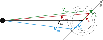
Figure 1. Schematic sketch of the velocity vectors of different solar wind components. Note that the depicted configuration is only for illustration purposes.
Download figure:
Standard image High-resolution imageAs can be seen, a variation of the IMF direction would lead to correlated or anticorrelated changes of the directions and magnitudes of velocities of all components in the spacecraft frame, whereas the velocity magnitudes remain constant in the suggested frame and their directions follow the magnetic field direction in this frame.
A ratio of the velocities of two different species, 1 and 2 measured in the spacecraft frame can be expressed as:
where θ is the angle between  and
and  . This equation is later used for a determination of the spacecraft frame velocity ratios under an assumption that differential velocities are aligned with the magnetic field by fitting the data measured for different magnetic field orientations.
The suggestion for the solar wind frame leads to several implications that can be tested experimentally, namely:
- 1.conservation of the magnitudes of differential speeds of all solar wind populations during the IMF rotation;
- 2.mitigation of a motional electric field for all populations; and
- 3.conservation of the total momentum in the solar wind frame.
The first criterion is a necessary condition for the existence of the suggested frame. We use data of Helios, Wind, ACE, and SOHO missions and show that differential speeds are conserved for all observable solar wind populations in Sections 4 and 5. The first considerations about a proper frame for a description of processes in the solar wind can probably be found in de Hoffmann & Teller (1950) in a connection with MHD shocks. They have shown the existence of a frame in which a plasma flows along the magnetic field and the motional electric field,  , is zero. For this reason, we will call the frame with
  de Hoffmann–Teller (HT) frame in further text. Although this frame is frequently used for a description of the particle motion at the magnetopause (e.g., Sonnerup et al. 1987; Hasegawa et al. 2005), around different types of discontinuities like interplanetary shocks (e.g., Neugebauer 2006) and in discussion of the shock drift acceleration of energetic particles (e.g., Webb et al. 1983); however, its application in the pristine solar wind is scarce.
Chao et al. (2014) used the HT analysis for a study of Alfvénic fluctuations but their analysis was based on an assumption that all solar wind species move with the same speed. Our scenario is more complex because we study a system with several components moving with their own speeds. Section 6 shows that the HT velocities computed from proton and alpha particle velocities are equal and an analysis of heavier ions reveals that the HT velocity derived this way can be applied to all components. Our investigations of the third criterion are presented in Section 7 but they lead to inconclusive results. We conclude our analysis with a discussion on interpretations and possible applications of the HT frame.
3. Experimental Support
The analysis combines the data of four missions:
- 1.
- 2.Helios 1 and 2 velocity distributions (Rosenbauer et al. 1977) with a ≈40.5 s time resolution and magnetic field (Musmann et al. 1975) observations averaged to the same time resolution as the plasma measurements. Our analysis revealed the importance of ion beams in the momentum balance but these data are not regularly available. For this reason, we revisited Helios measurements of the full 3D distributions and processed them with a motivation to determine parameters of the proton core and proton beam as well as those of alpha particles. The present study uses high-speed wind observations near the L1 point only; details of new Helios data processing can be found in Durovcova et al. (2019b).
- 3.Both SWICS (Gloeckler et al. 1998) and SWEPAM (McComas et al. 1998) ACE plasma instruments, and the magnetic field (Smith et al. 1998). The parameters of heavier ions (oxygen, iron) are based on the SWICS measurements of reduced 1D velocity distributions measured approximately along the Sun–Earth line with a 12 minute cadence. Since the differential velocities are directed along the magnetic field, long intervals with a predominantly radial IMF orientation were selected and specially processed for the present study.
- 4.The CTOF mass spectrometer as a part of the CELIAS instrument (Hovestadt et al. 1995) on board SOHO is designed to measure the kinetic properties and elemental/ionic compositions of solar wind ions with a cadence of ≈5 minutes. In addition, the CELIAS Proton Monitor (Ipavich et al. 1998) provides the solar wind proton mean speed and thermal velocity at a cadence of 30 s.
Note here that all proton and alpha particle parameters determined from the SWE (Wind) and SWEPAM (ACE) instruments used full 3D ion energy distributions and bi-Maxwellian fits are accessible via https://cdaweb.sci.gsfc.nasa.gov/. On the other hand, low densities of heavier ions cause several limitations that should be taken into account:
- 1.Both SWICS and CTOF instruments measure reduced 1D velocity distributions of all major heavy ions.
- 2.While SWICS also detects the 1D VDFs of alpha particles and protons, CELIAS/CTOF does not measure protons and also systematically cuts off the alpha particle VDFs, thus no reliable measurements of the alpha velocity can be obtained from CELIAS.
- 3.Due to the respective measurement principles and large differences in abundance between the ion species, the most reliable average velocities could be determined for alpha particles, oxygen (O6+) and iron (Fe9+, Fe10+) in the case of SWICS as well as oxygen (O6+), silicon (Si7+, Si8+), and iron (Fe9+, Fe10+, and Fe11+) in the case of CELIAS/CTOF.
- 4.The cadence (i.e., the time per one measuring cycle) of the heavy ion measurements is 12 minutes for SWICS and 5 minutes for CELIAS/CTOF. However, due to relatively narrow solar wind VDFs compared to the overall scanned velocity range, each ion VDF is scanned within a considerably smaller fraction of this time period (i.e., ≈1 minute).
Since none of the mentioned missions provides all necessary data with a sufficient time resolution, we are forced to combine the data from different instruments and missions, but this brings some problems that are demonstrated in two following figures. The heavy ions are measured only in the direction from the Sun and therefore we tried to identify the intervals of a radial IMF in the fast solar wind. However, these two conditions are in some sense contradictory because the radial IMF is usually connected with regions behind CIRs where the speed is usually low (Pi et al. 2014).
Figure 2 shows a 9 hr long (2003 October 7) interval of simultaneous Wind and ACE observations in a moderately fast quiet solar wind. Although plasma parameters and the IMF magnitude do not exhibit any systematic change, the IMF direction is strongly modulated by Alfvénic fluctuations of large amplitudes that are typical for the fast solar wind (Belcher & Davis 1971; Bruno et al. 1985; Smith & Balogh 1995; Matteini et al. 2014). Separation of the spacecraft along the YGSE axis was lower than 30 RE, thus one would expect that measured quantities would differ only due to high-frequency components of turbulence. This is more or less true for the proton density in the top panel but the alpha densities differ by a factor of 1.5 and also proton speeds are significantly different. The difference between ACE and Wind proton speeds is as large as a difference between the speeds of proton and alpha components determined from the Wind data. This example shows that the data from the different spacecraft cannot be simply combined.
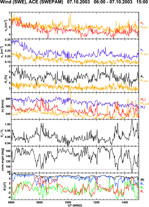
Figure 2. Example of Wind and ACE solar wind observations in front of the CIR on 2003 October 7. From top to bottom: the proton density; alpha density; a ratio of alpha to proton densities expressed in percent, AHe; proton and alpha speeds in the spacecraft frame; a ratio of proton to alpha speeds; the angle between the proton velocity and IMF (cone angle); IMF magnitude and its components. Note that ACE and Wind data are colored in the first four panels; the last three panels present only Wind measurements.
Download figure:
Standard image High-resolution imageThe ratio of proton and alpha speeds (fifth panel) varies from 0.95 to 1.02 and these variations are roughly anticorrelated with changes of the angle between the proton velocity and IMF vectors (cone angle hereafter, sixth panel). Variations of the speed ratio are consistent with the sketch in Figure 1 because this ratio is lowest when the velocity and IMF are about antiparallel (sixth panel), whereas it is close to unity if these vectors are perpendicular (compare fifth and sixth panels).
Velocities of different ion species registered by ACE with a lower time resolution through a prolonged time interval from the previous example are shown in Figure 3. The top panel shows the speeds of protons, alpha particles, oxygen and iron ions in various ionization states marked by different colors. Note that the proton speed shown in red was computed from the reduced velocity distribution measured by SWICS, while the velocity marked as P and highlighted by the black line was determined by fitting a proton part of the full 3D distribution measured by SWEPAM. The second and third panels present differential speeds computed with respect to the proton SWEPAM speed (second panel) and with respect to the proton speed determined from the SWICS data that will be considered in the further analysis (third panel). It can be seen that all differential speeds exhibit a similar magnitude and their changes are correlated with the IMF cone angle (fourth panel in Figure 3).

Figure 3. ACE observations of heavy ions for a longer time period (2 days): 2003 October 7–8. From top to bottom: different colors code the speeds of analyzed species in the spacecraft frame from SWICS that are complemented with the SWEPAM proton speed, P; differences between the SWEPAM proton speed and speeds of all species from SWICS; differential speeds of heavier species from SWICS; the cone angle; and the IMF magnitude. Hydrogen, helium, oxygen, and iron ions in different ionization states are shown.
Download figure:
Standard image High-resolution image4. Conservation of Magnitudes of Differential Velocities
The correlation between the differential speed and cone angle is demonstrated in Figure 4 where the  ratios for alpha particles, silicon, oxygen, and iron ions are plotted as a function of the IMF cone angle. Since the data are very noisy, the black bars represent medians in 10° bins of the cone angle. All ratios are close to unity for a 90° cone angle and decrease as the cone angle approaches 0° or 180°. This trend is highlighted by the fits based on Equation (4) and shown by the black curve in each panel. The top panels show the ACE data (Figure 4(a)), while SOHO observations are given in the bottom part (Figure 4(b)). It should be noted that both these observations have some limitations because ACE has a worse counting statistics due to a lower geometrical factor, while SOHO does not carry a magnetometer. To overcome this difficulty, we have computed the cross-correlation of Wind and SOHO proton speeds around each SOHO measuring point and used the determined time lag for the assignment of the Wind magnetic field to SOHO locations. Since differential velocities are small, we compare the velocities of heavier species with the proton velocity measured by SWIX to avoid the problem of inter-calibration of different instruments for ACE data but we should use the proton monitor in the case of SOHO because even the speed of alpha particles cannot be reliably determined from the CTOF measurements.
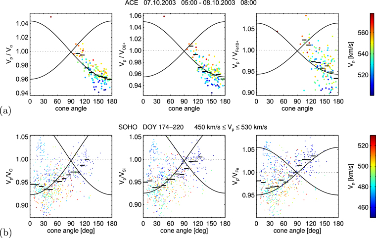
Figure 4. Ratios of the speeds of different solar wind components in the spacecraft frame as a function of the cone angle. The top panels analyze ACE observations shown in Figure 3. (a) The top panels show the proton core vs. alpha particles (left); the proton core vs. oxygen (middle); and the proton core vs. iron (right). (b) The bottom three panels present SOHO observations for DOY 174-220, 1996 in the fast solar wind and show the proton core vs. oxygen (left); the proton core vs. silicon (middle); and the proton core vs. iron (right). The black segments denote medians in the cone angle bins, whereas the black curves correspond to best fits using Equation (4).
Download figure:
Standard image High-resolution imageBoth mentioned limitations lead to a decrease of determined differential speeds but heavier species are clearly faster than protons and the Vp,SC/Vi,SC ratio can be as low as 0.9. The fits based on Equation (4) shown in all panels provide the following values of the velocity ratios: for the ACE data, Vp,SC/Vα,SC = 0.96; Vp,SC/VO,SC = 0.95; Vp,SC/VFe,SC = 0.94; Vp,SC/VO,SC = 0.92; Vp,SC/VSi,SC = 0.92; and Vp,SC/VFe,SC = 0.95 for the SOHO data. The SOHO ratios are medians for several ionization states of silicon or iron ions. We can conclude that the behavior of all populations is analogous to that described by Berger et al. (2011) and it is consistent with the sketch in Figure 1. This means that the magnitudes of differential velocities of heavy ions are conserved in course of the IMF rotation.
5. Statistical Study of Differential Speeds
The problem of noisy data can be partly overcome by a statistical processing. Marsch et al. (1982) has shown that the differential speeds of protons and alpha particles are roughly proportional to the proton bulk speed and this fact facilitates the statistical study that combines data from different time intervals. Unfortunately, scarce data with a sufficient time resolution do not allow us to do it for heavier ions but we did it for proton and alpha components using the Helios data measured between 0.7 and 1 au.
A great majority of the available proton and alpha particle velocities is gathered from the measurements of the full 3D ion energy distribution function without a mass selection. The parameters of different populations are estimated either by computations of the moments in energy ranges determined under an assumption that all species move with the same speed or by fitting the measured data with a sum of (bi-)Maxwellian distributions. However, the populations are overlapped in an angular/energy space due to their finite temperatures and the counts (currents) in a particular bin combine two or more populations. This feature is especially important when one tries to separate protons into the core and beam in a systematic way because the beam lies between proton and alpha components in the energy scale (Goldstein et al. 2000; Matteini et al. 2013). In order to reliably distinguish three basic populations (the proton core, proton beam, and alpha core), we reprocessed the Helios data because not only counts but also the currents were measured. This provides additional information that helps us to separate the different ion populations.
Figure 5(a) uses the already mentioned fact that the differential speeds are roughly proportional to the proton speed and presents the ratios of speeds of the proton core, proton beam, and alpha core determined in the spacecraft frame as a function of the cone angle. The color scale marks the observation probability in each cone angle bin, the black lines present fits corresponding to Equation (4). An extrapolation of the maximum probability to zero cone angle provides the following ratios: Vp,SC/Vpb,SC = 0.86; Vp,SC/Vα,SC = 0.92; and Vα,SC/Vpb,SC = 0.92. These numbers show that (in the fast solar wind) the slowest of investigated populations is the proton core and the alpha particle speed is in the middle between the proton core and beam. In order to stress the constant differential speeds over the magnetic field rotation, Figure 5(b) shows the proton beam and alpha core velocities in the proton core frame. Note that the vertical axes present the magnitudes of the differential velocity projected onto instantaneous magnetic field direction to decrease the fitting errors.
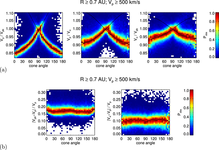
Figure 5. (a) Probability of Helios observations of ratios of the speeds of solar wind components as a function of the cone angle; (left) the ratio of the proton core and proton beam; (middle) the ratio of the proton core and alpha core; and (right) the ratio of the alpha core and proton beam. Note that the ratios are computed from velocities larger than 500 km s−1 measured in the spacecraft frame. (b) The velocities of the proton beam (left) and alpha core (right) normalized to the proton core speed in the spacecraft frame.
Download figure:
Standard image High-resolution imageThe data presented in this section clearly demonstrate that the differential speeds of all analyzed species are constant in course of the IMF rotations. It should be noted that we have investigated the relative motion of different populations with respect to the protons because their parameters are most precisely determined, but an analogous picture would be seen if we had used any other population as a base.
6. De Hoffmann–Teller Frame
The principal question is whether the HT velocities determined for particular species are identical. To find such a frame, we have searched for a velocity, VHT, that minimizes the electric field, 
where  (tj) is the velocity of a given ion population measured in the spacecraft frame at a time tj,
  is the in situ magnetic field measurement at tj within a period of ΔT. The procedure requires a large number of simultaneous measurements of velocity and magnetic field vectors made within a shortest possible time to reflect the expected VHT variations. As a compromise, our initial search uses ΔT = 60 minutes of the Wind measurements and the resulting VHT value was attributed to the center of the interval. The interval was then shifted by one time step of plasma measurements and the procedure was repeated.
A demonstration of the results of this procedure is shown in Figure 6. The event chosen for a demonstration is characterized by Alfvénic fluctuations with large amplitudes. The first panel shows that the protons in the spacecraft frame oscillate in accord with IMF variations, while helium ions keep the decreasing trend without any significant modulation by the IMF cone angle (fourth panel). The fifth panel demonstrates the crucial results of our analysis—the HT velocities computed from protons and alpha particles are about identical. The proton and alpha speeds in the HT frame (last but one panel) are changing smoothly; no modulation by the IMF cone angle is seen. The dotted line in this panel uses the VHT computed from alpha particles and we can note that the differences are hardly visible.
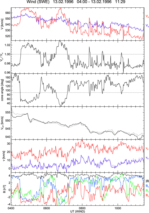
Figure 6. Example of applications of the HT frame to the Wind data (1996 February 13). From top to bottom: proton and alpha velocities in the spacecraft frame; differential speed normalized to the Alfvén speed; the ratio of proton and alpha speeds in the spacecraft frame; the HT velocity computed from the proton (full line) and alpha (dotted) velocities; proton and alpha velocities in the HT frame; IMF magnitude and its components. All parameters are derived from Wind observations.
Download figure:
Standard image High-resolution imageSince the results in Figure 6 are encouraging, we have carried out a statistical study based on a full set of the Wind data. In order to estimate the influence of the interval length, we repeated all analyses also for 20 minute intervals. As could be expected, an extension of the time interval enlarges slightly the residual electric field but the results for the HT velocity computed from protons and alpha particles are the same as demonstrated in Figure 7(a). An answer to the principal question, whether VHT determined from protons and alpha particles are identical can be found in Figure 7(b) showing their ratio. This ratio is close to unity; the differences are typically lower than 3 × 10⁻³, which is well within the measurement errors. We are searching for a frame where also the electric field of fluctuations vanishes. The computation of VHT on 1 hr interval cannot reflect fluctuations faster than 3 × 10⁻⁴ Hz, thus we are using VHT determined on 20 minute intervals hereafter.

Figure 7. (a) Histograms of the residual electric field in the HT frame determined from proton (full line) and alpha particle (dotted line) velocities on 1 hr (red) and 20 minute (blue) intervals. (b) Histograms of ratios of HT velocities determined from proton and alpha particle velocities on 1 hr (red) and 20 minute (blue) intervals (Wind).
Download figure:
Standard image High-resolution imageA probability of observations of proton and alpha particle speeds in the HT frame is shown by 2D histograms in Figure 8. Note that Vp and Vα in these panels are a projection of the velocities onto an instantaneous IMF direction in order to minimize the influence of fast IMF variations, and the sign of the speed indicates whether the velocities are parallel or antiparallel to the ambient magnetic field.

Figure 8. Probability maps of simultaneous Wind observations of proton, Vp, and alpha, Vα speeds in the HT frame in the slow (left) and fast (right) winds. VHT was computed on 20 minute intervals from the proton velocity. The dashed black lines in both panels stand for equality of both speeds. Only data with the residual electric field below 6 mV m−1 are plotted.
Download figure:
Standard image High-resolution imageA comparison of two panels in Figure 8 shows distinctly different behavior of the speeds of both species in the slow and fast winds. Taking into account the measurement uncertainty, the speeds do no exceed the Alfvén speed but, whereas speeds of both populations are about equal in a collisionally older slow wind, the speed of alpha particles is very small in the fast wind. A small portion of observations of very low proton speeds can be attributed to measurements within coronal mass ejections (Durovcova et al. 2017). Note that the velocity distributions are often strongly anisotropic and thus we use the Alfvén speed corrected for the temperature anisotropy.
The HT frame would be a frame of the dominant perturbations which are typically Alfvénic in the fast solar wind (Chao et al. 2014). Matteini et al. (2015) analyzed one event and showed that their observations can be interpreted as alpha particles standing in the fluctuation frame. The proton velocity in such a frame keeps its magnitude (about equal to the Alfvén speed) but its direction changes in phase with the magnetic field rotation. In order to check if such behavior is typical, four panels of Figure 9 show a relation between speeds of analyzed populations in the HT frame and Alfvén speed. The medians in the velocity bins depicted as heavy black lines in the left panels show that the speeds of both protons and alpha particles are typically about half of the Alfvén speed in the slow solar wind. The situation is closer to that described by Matteini et al. (2015) in the fast wind (right panels) but the speed of alpha particles is nonzero in a systematic manner.
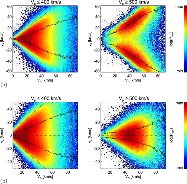
Figure 9. Probability maps of proton (top) and alpha (bottom) speeds in the HT frame as a function of the Alfvén speed in the slow (left) and fast (right) solar winds. The black full lines mark medians in positive and negative velocity sectors; the dotted lines show the relations Vi = ±VA.
Download figure:
Standard image High-resolution imageFigure 10 presents the same data as previous figures but as a function of the cone angle. Note that a probability color scale is linear in this case in order to emphasize the dynamics. The surrounding line plots show the probability as a function of a single parameter. The medians depicted by the black lines indicate that all normalized speeds are about constant and switch the sign when the proton velocity in the spacecraft frame and the magnetic field become perpendicular. The magnitudes of velocities of both species are about equal (≈0.4 VA) in the slow solar wind but the speed of alpha particles can be considered as a proxy of VHT in the fast wind. The negative velocities at small cone angles mean that both populations move generally sunward in the HT frame.

Figure 10. Probability maps of observations of proton (top panels) and alpha (bottom panels) speeds in the HT frame as a function of the cone angle in the slow (left) and fast (right) streams. VHT was computed on 20 minute intervals from the proton velocity. The black lines show the medians of particular speeds in cone angle bins. The line plots surrounding the color panels are 1D histograms showing the probability as a function of the single parameter.
Download figure:
Standard image High-resolution imageThe question of whether the difference between the fast and slow wind is connected with their different origin in the solar corona or it is formed during a propagation through the interplanetary space will be addressed in the follow-up study. We will concentrate on the behavior of different ion species in the fast wind in the further analysis.
7. Total Momentum in the HT Frame
Our analysis reveals that the protons generally move sunward in the HT frame and their momentum would be compensated by the momentum of other species if our assumption on the momentum balance (Equation (3)) is valid. Taking into account the result that Vα,SC is a good approximation of VHT, we analyzed the momentum in the alpha frame. The momentum of alpha particles is thus zero and Figure 11, covering the same interval as Figure 4, shows that heavier species (oxygen and iron ions taken from ACE) are only slightly faster than alpha particles; the fits lead to the following values Vα,SC/VO = 0.99; Vα,SC/VFe,SC = 0.97. Taking into account that the total mass of species heavier than helium is up to 1% of the proton mass, their contribution to the overall momentum is probably very small.

Figure 11. Ratios of the speeds of different solar wind components as a function of the cone angle; (left) oxygen vs. alpha particles; (right) iron vs. alpha particles (ACE data).
Download figure:
Standard image High-resolution imageThe only investigated population moving clearly antisunward in the HT frame is the proton beam. Thus, we used Helios observations above 0.7 au and calculated the proton beam and proton core velocities relative to the velocity of alpha particles as well as densities of these two populations (Durovcova et al. 2019a). Figure 12 compares their momenta (in arbitrary units) and shows that the proton beam can balance typically about 10% of the core momentum in the alpha frame (heavy line) but the beam momentum can frequently reach 40%–50% of the core momentum.
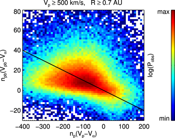
Figure 12. Probability map of simultaneous Helios observations of the proton beam and core momenta. The black line stands for the relation npb · (Vpb − Vα) = −0.1npc · (Vp − Vα).
Download figure:
Standard image High-resolution image8. Summary and Discussion
The presented analysis of observations based on the data of four spacecraft revealed the following:
- 1.The magnitudes of differential velocities of solar wind ion components are approximately constant on scales of hours.
- 2.The vectors of differential speeds are aligned with the magnetic field vector and rotate with it.
- 3.This rotation is observed as variations of the speeds of these components in the spacecraft frame that are correlated with the IMF rotation.
- 4.De Hoffmann–Teller velocities computed from protons and alpha particles are equal and the residual electric field typically does not exceed 1 mV m−1. This means that the HT frame is well defined. VHT does not depend significantly on a duration of the intervals used for its determination; shorter intervals result in a smaller residual electric field.
- 5.
- 6.The same is true for the speed of alpha particles, the proportionality constants are 0.1 in the fast and ≈0.4 in the slow wind. From this it follows that the velocity of alpha particles in the spacecraft frame is a good approximation of VHT in the fast wind.
- 7.In the slow solar wind, the velocities of protons and alpha particles in the HT frame are equal within the measurement uncertainties.
- 8.The velocities of heavier solar wind components are very close to the velocity of the alpha particles.
All these findings are in line with our suggestion shown in Figure 1, if we put VSW = VHT. However, the experimentally determined total momentum is not zero in the HT frame—the momentum of the proton beam is much lower than that of the proton core and momenta of all other analyzed species are too small to compensate a difference between the proton core and proton beam momenta.
We should admit that the frame of zero total momentum (fluid frame) and the HT frame could be different. Since a plasma motion across the magnetic field would result in the parallel electric field, let us expect that the mutual velocity of these two frames is oriented along the mean magnetic field. However, the HT frame is unique (Khrabrov & Sonnerup 1998), thus any transformation along the magnetic field would enlarge the motional electric field and the resulting  drift would return the plasma back into the HT frame. This mechanism is consistent with our finding that VHT can be determined from proton as well as from alpha velocities, thus we propose the HT frame as a proper frame for investigations of processes in the solar wind. A brief discussion on the relation between the HT velocity and the velocity of waves propagating in the solar wind can be found in the Appendix.
However, a determination of the total momentum suffers several experimental limitations:
- 1.VHT in the present study was determined on the timescale of 20 minutes but the magnetic field can rotate over a large angle during this time. The determined velocity Vi = Vi,SC − VHT thus differs from its proper value.
- 2.Variations of the IMF cone angle during the interval of the measurements of a particular distribution lead to underestimation of Vi, and this effect increases with the decreasing time resolution.
- 3.We are not able to determine the parameters of beams of heavier species; even the proton beam can be reliably estimated only if it is intense and the temperatures of protons and alpha particles are low enough.
- 4.The core-beam structure of heavier species can be seen only if the accumulation time is sufficiently long and corresponding densities of particular populations are high.
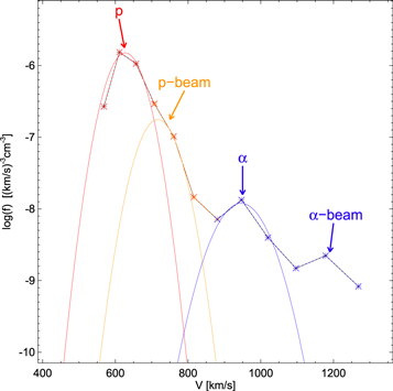
Figure 13 presents one example of the detailed analysis of the Helios spectrum with fits of proton and alpha core, and proton beam. The points represent values measured in one of the angular sectors but the colored lines show fits of particular ion populations (proton core and beam, alpha core, and beam) using a full measured 3D distribution. The figure clearly demonstrates also a presence of the alpha beam. Identification of beams of heavier species that are measured only in the Sun–Earth direction would require long intervals of a stable radial IMF but such intervals can be encountered nearly exceptionally in the slow solar wind that is collisionally old, differential speeds are thus low and the core-beam structure is hidden. If we expect that the beams of all species behave similarly (i.e., they are faster than the corresponding core, the difference between core and beam velocities is about Alfvén speed and the beam density is 10%–20% of the corresponding core density), the momentum of beams is not sufficient to balance the total momentum.
Figure 13. Demonstration of the alpha beam in the Helios energy distribution. The horizontal axis is in units of the proton velocity, Vp; the crosses stand for the measured data; red and blue colors show the points with dominant proton and alpha contributions, respectively. The color curves show Maxwellian fits of three distinguished populations (proton core, alpha core, and proton beams). Note that the α-beam is clearly visible, but not fitted.
Download figure:
Standard image High-resolution image
Moreover, the real ion velocity distribution is very complicated and our treatment using several Maxwellian populations is a crude simplification. A step forward would be an involvement of the temperature anisotropy of all species into the momentum balance but the principal problems connected with limitations of the spacecraft experiments remain.
9. Conclusion
Our analysis of relative drifts of different ion populations driven by a motivation to find such a frame that provides the easiest description of the observed experimental results shows the following:
- 1.The HT frame can be generalized for applications in the solar wind multicomponent plasma.
- 2.The HT velocities determined from the velocities of different populations in the spacecraft frame of reference are identical.
- 3.The velocities of all analyzed species are aligned with the magnetic field in the HT frame.
- 4.The HT frame can be considered as a proper solar wind frame, although the momentum conservation remains under critical debate.
- 5.The velocity of the core of the alpha particle distribution, Vα,SC, is a good approximation of VHT in the fast wind, but not in the slow wind.
Last but not least, we should stress that the HT frame can be applied only for a detailed analysis, locally and within a particular solar wind stream. The crossings of boundaries of different solar wind streams result in changes of differential speed magnitudes. For example, Durovcova et al. (2019a) clearly demonstrated that the differential speed of protons and alpha particles can fall to zero during the crossings of the stream interaction region even in the fast solar wind.
A more detailed analysis of the effects discussed in this paper could be directed to the space missions as Parker Solar Probe and Solar Orbiter that are realized or planned.
The authors acknowledge the spacecraft teams (Helios, Wind, ACE, SOHO) for the data available via http://cdaweb.gsfc.nasa.gov/. The present work was supported by the Czech Science Foundation under Contract 19-18993S and Charles University Grant Agency under No. 1484217.
Facilities: Helios - , Wind - , ACE - , SOHO. -
Appendix: The Relation Between the HT Frame and Waves in the Solar Wind
Let us assume a homogenous plasma with the frozen-in magnetic field,  . If this magnetic field is constant in space and time, the electric field
  is zero in each frame moving with a velocity,
  , along this field and thus all such frames can be considered as HT frames. However, this situation is far away from conditions in the solar wind because the Sun launches a variety of waves. If the magnetic field is modulated by a single Alfvén wave (Webb et al. 2010) or even double wave (Webb et al. 2012) propagating along
  , there is only one frame with
  the frame moving with the wave. Such a situation can be often encountered in the fast solar wind as our Figure 6 or the case studied by Matteini et al. (2015) demonstrate.
When the fluctuations are not purely Alfvénic, the frame where  does not necessarily exist but we can still search for a frame where
  acquires its minimum, using Equation (5). The value of the residual field would depend on the length of an interval used for the HT frame determination because one value of the HT velocity is attributed to a whole interval. Our analysis (Figure 7(a)) shows that
  is typically very small, approximately in the order of 0.1 mV m−1. For an usual IMF value of 10 nT, it corresponds to about 10 km s−1 uncertainty in the frame determination and this value is comparable with the high-frequency noise in the velocity and magnetic field measurements.
It can be easily shown that the HT velocity is proportional to the unperturbed magnetic field component and does not depend on the wave amplitude in the case of a single linear Alfvén wave. However, it is a question of what would be the HT velocity in a model case of two oppositely propagating waves. The solar wind carries plenty of wave modes propagating in different directions including the sunward waves generated by a reflection of the originally antisunward propagating waves at different discontinuities. Chandran & Perez (2019) have shown that an interaction of counter-streaming waves is one of the sources of solar wind turbulence but they did not address the problem of the motional electric field in their simulations (see also Howes 2015, 2016).
A majority of theoretical studies of waves in the solar wind is based either on the MHD approach or kinetic simulations but there are only several papers dealing with multiple ion species. Zhao et al. (2013) studied a parametric instability of kinetic Alfvén waves and have shown that the presence of heavy ions stabilizes its growth rate. Li & Li (2009) analyzed theoretically the earlier Helios observations of the transfer of angular momentum from the Sun to the interplanetary space assuming that the solar wind composed of protons and alpha particles. In order to account for their differential motion, the authors used center-of-mass frame. To our knowledge, none of published studies of multiple species behavior deals with the effects of the motional electric field and there is room for future theoretical effort. It should be based on the ion kinetics because our analysis has shown that a description of the solar wind as an ensemble of several Maxwellian populations is probably not sufficient. In spite of this limitation, we have shown that the HT velocities determined from proton and alpha particle velocities are equal (Figure 7(b)) and it stresses the importance of the HT frame for studies of solar wind processes.