


Abstract
We have mapped the young Herbig Be star R Mon in CO(3–2) and 13CO(3–2) with Atacama Pathfinder EXperiment in Chile and analyzed unpublished Herschel images. We find that R Mon is embedded in a small cloud with a gas temperature of ∼20 K and a total mass of ∼70  . We confirm that R Mon drives a bipolar molecular outflow, which is blueshifted north of R Mon. The blueshifted outflow has excavated the molecular cloud north of R Mon, creating the reflection nebula NGC 2261 and filling it with high-velocity gas. At "high" velocities the orientation of the outflow is approximately n–s, which agrees with the optical jet, suggesting that the accretion disk is e–w. The outflow velocities are modest, ±9 km s−1. The outflow is rather massive, ∼0.56
  in the blueshifted outflow lobe. The outflow is completely optically thick in CO(3–2) toward R Mon, indicating that its envelope is ≲2000 au. The mass of the accretion disk and surrounding envelope determined from an isothermal graybody fit is ∼0.34
  . We estimate a mass-loss rate of ∼(1–3) × 10−5
  yr−1, corresponding to an accretion rate of (1–9) × 10−6
  yr−1. We find that R Mon has bolometric luminosity of <1000
  . R Mon is still in an active accretion phase, contributing to the observed luminosity. Hence, R Mon cannot be a B0 star; it must be a late B star or even an early A star.
Export citation and abstract BibTeX RIS
1. Introduction
R Mon is a young Herbig Ae/Be (HAEBE) star (Herbig 1960) illuminating a fan shaped nebula, NGC 2261. Hubble (1916) found that NGC 2261 showed clear variations in brightness and morphology on timescales from months to years; hence, it is often referred to as Hubble's Variable Nebula. These brightness variations have been explained as being due to dust clouds close to R Mon, which move around the star causing shadows on the walls of the conical reflection nebula (Bellingham & Rossano 1980; Lightfoot 1989). R Mon is located at the northern rim of a small dark cloud about 1° from the young cluster NGC 2264 and assumed to be at the same distance as the cluster, i.e., ∼800 pc (Jones & Herbig 1982). This agrees within errors with the distance estimated by Close et al. (1997), 760 pc. The spectral type for R Mon is uncertain. Cohen & Kuhi (1979) assigned it a spectral type of B1 with an AV = 3.5 mag by decomposition of the spectral energy distribution (SED). Hillenbrand et al. (1992) assigned it a spectral type of B0 with an AV = 4.3 mag, while Mora et al. (2001) classified it as B8 IIIe. R Mon powers a faint thermal radio jet, 0.29 ± 0.03 mJy at 6 cm (Skinner et al. 1993) with a spectral index, α = 0.9 ± 0.4, consistent with wind excited free–free emission. The star powers a collimated high-velocity jet (Brugel et al. 1984; Movsessian et al. 2002) and is believed to be the exciting star of the Herbig–Haro complex HH 39, 7 5 north of R Mon (Herbig 1974; Cantó et al. 1981; Jones & Herbig 1982). The high-velocity jet is very bright in [S ii] (Movsessian et al. 2002). The northern blueshifted jet has about constant intensity up to about 5'' from R Mon and then the intensity drops abruptly. The velocity of the inner jet is −93 km s−1. The velocity is still −90 km s−1 at the second knot 9'' to the north. At the northern tip, 14'' from R Mon, the velocity has dropped to −54 km s−1. The southern counter jet has a bright knot about 5'' to the south with a velocity of +108 km s−1 and terminates in a Herbig–Haro like knot 18'' to the south with a velocity of +184 km s−1. Movsessian et al. (2002) resolve the jet and find a width of about 2
 5. There is a clear velocity gradient over the jet, up to 70 km s−1, suggesting that the jet is rotating. Böhm & Catala (1994) detected forbidden [O i] 6300.31 Å emission toward R Mon, where it is seen as an asymmetric, blueshifted line (−114 km s−1, full width a zero intensity) with hardly any redshifted emission.The [O i] 63 μm line is very strong (Riviere-Marichalar et al. 2016; Jiménez-Donaire et al. 2017). Riviere-Marichalar et al. (2016) fitted the [O i] line with a three velocity component Gaussian resulting in a redshifted velocity component at +126 km s−1, a blueshifted one at −219 km s−1, plus a rest frame velocity component, which dominates the line intensity. Such high jet velocities appear unrealistic. The highest velocities seen in optical lines like [S ii], which are far easier to excite than [O i] 63 μm, are about 100 to at most 120 km s−1. Therefore the high [O i] 63 μm velocities found by Riviere-Marichalar et al. must be instrumental or artifacts from the fitting procedure.
R Mon is a binary system with the companion being a late T Tauri star with a separation of 07 (Close et al. 1997). It was detected in the submillimeter continuum by Mannings (1994) and in mm-continuum with the Plateau de Bure Interferometer (PdBI; Fuente et al. 2003). Fuente et al. (2006) used the PdBI to image R Mon in CO(1–0) and (2–1) and interpreted their results as Keplerian rotation around an 8  star. In a follow-up study by Alonso-Albi et al. (2018) they revisit R Mon with additional PdBI data and PACS spectroscopy and argue that R Mon is a B0 star (8
  ) surrounded by a Keplerian disk with an inner gap, i.e., a transition disk. However, their modeling ignores the molecular outflow and any contribution from accretion onto R Mon, which, if included, would change their results.
R Mon drives a molecular outflow (Cantó et al. 1981). Even this outflow was one of the first molecular outflows discovered from a HAEBE star, there are no new published maps of the R Mon outflow since the pioneering study by Cantó et al. (1981). Here we present recently acquired CO(3–2) and 13CO(3–2) maps of R Mon with a spatial resolution of ∼18'' obtained with the 12 m Atacama Pathfinder EXperiment (APEX4 ) in Chile. With APEX we have also obtained long integration spectra in CO(2–1), 13CO(2–1), and C18O(2–1) as well as 13CO, 12CO(3–2), and 12CO(4–3). Analysis of these data sets enables us to characterize the molecular outflow and its relation to the Hubble variable nebula, NGC 2261. Additionally we analyze unpublished Herschel Space Observatory PACS and SPIRE images of R Mon, which allow us to put constraints on the spectral type of R Mon.
2. Observations
2.1. APEX
R Mon was mapped on 2018 December 8 in good weather conditions (precipitable water vapor, pwv = 0.71 mm) in 13CO(3–2) and 12CO(3–2) using the 7 pixel LAsMA array on APEX in Chile (Güsten et al. 2006). LAsMA is a 7 pixel single polarization heterodyne array tunable from 270–370 GHz. The array is arranged in a hexagonal configuration around a central pixel with a spacing of about two beam widths between the pixels. It uses a K mirror as de-rotator. The backends are the new Fast Fourier Transform fourth Generation Spectrometers (Klein et al. 2012) with a bandwidth of 2 × 4 GHz. We observed 12CO(3–2) and 13CO(3–2) by placing 12CO in the upper sideband and 13CO in the lower sideband. The mapping was done in total power on-the-fly mode using a clean reference position, +120'', −2050'' relative to R Mon. We mapped a region of 65 × 72. The map was scanned in both R.A. and decl. with a spacing of 6'', resulting in a uniformly sampled map with good fidelity. The data were reduced using CLASS.5
All spectra are calibrated in Tmb, see Table 1.
Table 1. Observation Details: Frequencies, Receivers, Half Power Beam Widths (HPBWs), Beam Efficiencies, and rms Sensitivities
| Receiver | Transition | Frequency | θHPBW | ηmb | rmsa |
|---|---|---|---|---|---|
| (GHz) | ( '' ) | (K) | |||
| PI230 | CO(2–1) | 230538.000 | 27.3 | 0.70 | 0.017 |
| 13CO(2–1) | 220398.684 | 28.5 | 0.70 | 0.014 | |
| C18O(2–1) | 219560.354 | 28.6 | 0.70 | 0.013 | |
| LAsMA | 13CO(3–2) | 330.587965 | 19.0 | 0.70b | 0.15c |
| CO(3–2) | 345.795990 | 18.2 | 0.70b | 0.13c | |
| FLASH+ | 13CO(3–2) | 330.587965 | 18.5 | 0.69 | 0.035 |
| CO(3–2) | 345.795990 | 17.7 | 0.69 | 0.025 | |
| FLASH+ | CO(4–3) | 461.040768 | 13.3 | 0.58 | 0.14 |
Notes.
aThe velocity resolution is 0.5 km s−1 for all spectra. bAverage for all pixels. cRms per resolution element, 91 × 91.
Download table as: ASCIITypeset image
Long integration spectra (16 minutes, on+off) of CO(2–1), 13CO(2–1), and C18O(2–1) in good weather conditions (pwv = 2.2 mm) were obtained on 2018 December 10 with the PI230 receiver on APEX. We observed two positions: one centered on R Mon and a second one on the bright far-infrared (FIR) peak at offset −40'', +58'' on the western side of NGC 2261. PI230 is a dual polarization, dual sideband receiver with good image band rejections. Each band has a bandwidth of 8 GHz and therefore each polarization covers 16 GHz. Each band is connected to two FFTS4G spectrometer (Klein et al. 2012) with 8 GHz bandwidth and 131,072 channels, providing a frequency resolution of 61 kHz, i.e., a velocity resolution of ∼0.079 km s−1 at 230 GHz. The PI230 receiver can be set up to simultaneously observe CO(2–1), 13CO(2–1), and C18O(2–1). Observations details are summarized in Table 1.
Long integration spectra (20 minutes) of CO(3–2), 13CO, and CO(4–3) were obtained with FLASH+ on APEX on 2018 December 12 of the same positions observed with PI230. The weather conditions for the CO(4–3) observations were marginal. Therefore these observations were repeated on 2019 April 18 in dry weather conditions (pwv = 0.8 mm). The integration time for the April observations was 20 minutes. FLASH+ is a dual channel heterodyne SIS receiver operating simultaneously—on orthogonal polarizations—in the 345 GHz and in the 460 GHz atmospheric windows. Both bands employ state-of-the-art sideband separating SIS mixers. The mixers provide large tuning ranges enabling us to simultaneously observe 13CO and 12CO(3–2) in the 345 GHz window and 12CO(4–3) in the 460 GHz window. The backends are FFTS4G spectrometers, proving a velocity resolution of 0.053 km s−1 at 345 GHz and 0.040 km s−1 at 461 GHz. The CO(3–2) spectrum is an average of the December and April observations. Observation details are summarized in Table 1.
2.2. PACS and SPIRE Imaging
We retrieved Herschel Space Observatory PACS and SPIRE imaging of R Mon from the Herschel data archive. The SPIRE imaging was obtained in Small Map mode with a scan speed of 30''/s on 2013 March 24 (OD 1411; AOR-ID 1342268324). The PACS imaging was done in cross scan mode with medium scan speed, 20''/s, for both 70/160 μm (AOR-IDs 1342269841 & 1342269842), and 100/160 μm (AOR-IDs 1342269843 & 1342269844). These observations were carried out on 2013 April 11 (OD 1428). Both the SPIRE and PACS observations were part of an OT1 program by G. Meeus (OT1_gmeeus_1). The half power beam widths (HPBWs) for PACS are 56, 68, and 113 for 70, 100, and 160 μm, respectively. For SPIRE the HPBWs are 184, 252, and 367 for the 250, 350, and 500 μ bands, respectively.
3. Results and Analysis
3.1. The R Mon Molecular Cloud
Cantó et al. (1981) mapped the R Mon region in CO(1–0) and found that R Mon is located in a small elongated molecular cloud, ∼0.8 × 0.4 pc. Based on their observations they argued that the stellar wind of R Mon has created a bipolar cavity, with blueshifted emission to the north and redshifted emission to the south. In their interpretation the conical nebula NGC 2261 is shining in light reflected from the cavity walls of the northern outflow, a view which is commonly accepted. They also found another small cloud ∼7' to the north of R Mon, where the outflow becomes visible as the Herbig–Haro complex HH 39. This cloud has a velocity of ∼7.5 km s−1, while R Mon has a Vlsr of 9.5 km s−1, i.e., they are separate clouds.
Our high spatial resolution CO(3–2) and 13CO(3–2) maps do not go far enough to the north to show the northern cloud. The SPIRE images, however, capture most of the northern cloud and HH 39, see Figure 1. The SPIRE images confirm that there is a region free of dust emission between the R Mon cloud and the HH 39 cloud.
Our high spatial resolution SPIRE and CO (3–2) images show that the cloud in which R Mon is embedded has a filamentary structure with one narrow filament running from NE to SW through R Mon and NGC 2261. A second filament extends at least 35 to the south from R Mon (Figures 1 and 2).There is another faint filament to the east of the southern filament, which is outside the area mapped in CO, see Figure 1. 13CO(3–2) is less extended than the 12CO emission. The southern filament is not seen at all in 13CO, suggesting that this part of the cloud has lower column density. The Hubble nebula stands out as a cavity in both dust and CO emission, with the western side being rather prominent both in dust and 13CO, while CO(3–2) is stronger on the eastern side of the nebula. It is likely that the CO(3–2) emission may be enhanced by the outflow at velocities close to the systemic velocity of the R Mon cloud.
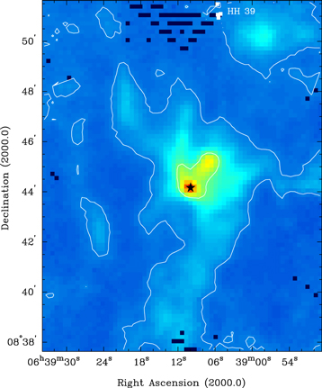
Figure 1. False color SPIRE 350 μm map showing the filamentary like cloud surrounding R Mon. The black blotches in the north are due to incomplete coverage of the SPIRE imager. A few more are seen toward the edges of the map. At the northwestern edge of the image we see a second cloud and the Herbig–Haro complex HH 39 at the northeastern edge of this cloud. We have plotted the HH objects HH 39 A, E, C, and D as filled white squares. A is at the top, D at the bottom. The position of R Mon is marked with a black star symbol The SPIRE image does not capture the total extent of the cloud to the west and to the south. The background level in the image is ∼0.56 Jy beam−1 with the peak flux density of 4.56 Jy beam−1. We have highlighted the image with two white contours levels. One, at 0.7 Jy beam−1, is showing the extent of the molecular cloud, while the other one, at 1.75 Jy beam−1, shows the dense gas cloud in which R Mon is embedded.
Download figure:
Standard image High-resolution image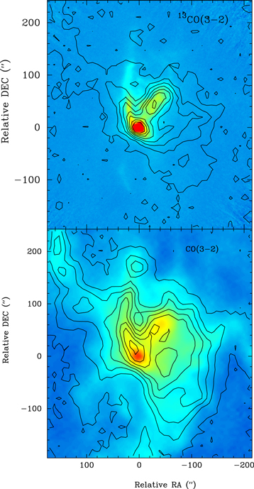
Figure 2. Contour plots of CO(3–2) and 13CO(3–2) integrated over 2 km s−1 wide velocity interval centered on 9.4 km s−1, showing the emission from the R Mon molecular cloud. The 13CO(3–2) map (top) is plotted with black contours overlaid on a PACS 100 μm image. At 100 μm the emission is completely dominated by R Mon and the Hubble variable nebula. Some faint emission is seen south of R Mon, almost certainly outlining the redshifted outflow to the south. The CO(3–2) map (bottom) is also plotted in black contours, but overlaid on a SPIRE 250 μm image with logarithmic stretch. The HPBWs of CO(3–1) and the SPIRE 250 μm image are almost identical (182 versus 184). The CO(3–2) emission follows the dust emission very closely.
Download figure:
Standard image High-resolution imageOne can see from the three-color image of the R Mon cloud (Figure 3) that the Hubble variable nebula is hotter than the surrounding cloud, which appears to have a relatively uniform temperature. To further characterize the cloud and the reflection nebula, we have done simple graybody fits (see e.g., Sandell 2000 and Section 4.2) using flux densities deduced from the PACS and SPIRE images. The flux densities for the cloud surrounding R Mon were integrated over the same area we mapped in CO(3–2) and 13CO(3–2) after subtracting emission from the reflection nebula. We also did a graybody fit of the warmer dust emission associated with the reflection nebula after subtracting out the emission from R Mon (Table 2). The graybody fit to the flux densities of the reflection nebula gives a dust temperature, Td = 31 K, and a dust emissivity. β = 1.38, resulting in a mass (gas + dust) of 2.6  , assuming standard Hildebrand dust opacity. For the surrounding cloud we derive Td = 18.7 K, β = 1.49, and a mass of 66
  , or ∼70
  in total.

Figure 3. Three-color image of R Mon/NGC 2261 and the surrounding molecular cloud. The SPIRE 250 μm is red, the PACS 160 μm is green, and the PACS 70 μm is blue. R Mon is the bright star at 0'', 0'', while the yellow and green emission outline the Hubble variable nebula, NGC 2261.
Download figure:
Standard image High-resolution imageTable 2. Flux Densities of R Mon (PACS and SPIRE) and Integrated Flux Densities within an 80'' Radius
| Filter | FWHM | Flux Density | Integrated flux |
|---|---|---|---|
| ( '' ) | (Jy) | (Jy) | |
| 70 | 5.6 | 52 ± 10 | 152 ± 23 |
| 100 | 6.7 | 33 ± 4 | 191 ± 29 |
| 160 | 11.3 | 18 ± 2 | 141 ± 21 |
| 250 | 18.4 | 7.4 ± 0.7 | 95 ± 10 |
| 350 | 25.2 | 3.6 ± 0.4 | 40 ± 4 |
| 500 | 36.7 | 1.3 ± 0.3 | 17.5 ± 2 |
Download table as: ASCIITypeset image
The long integration spectra toward R Mon were fit with two-component Gaussians, while only one velocity component was needed for the FIR peak. The results of these Gaussian fits are given in Table 3. Using the equations given in Nishimura et al. (2015) we can now use these results to derive gas temperatures and column densities of CO and its isotopologues. Nishimura et al. only discuss CO(2–1) and its isotopologues, but we have expanded them to higher J-transitions of CO using the generalized derivations for how to calculate column densities presented in Mangum & Shirley (2015). CO(2–1) gives a gas temperature of 20 K for the cloud emission both toward R Mon and the FIR peak. This is in good agreement with the dust temperature, 18.7 K, derived from the graybody fit. We find that 13CO(2–1) is significantly optically thick at both positions. The 13CO(2–1) optical depth of the molecular cloud is 0.74 toward the FIR peak and 0.76 toward R Mon. C18O(2–1) is essentially optically thin with optical depths of 0.05 and 0.07 toward R Mon and the FIR peak, respectively. 13CO(3–2) is optically thick in the dense compressed gas surrounding the outflow. Toward R Mon the optical depth is 1.55, although it is possible that the 13CO peak emission could include some of the outflow. Toward the FIR peak the optical depth is 0.66, i.e., more similar to the 13CO(2–1) optical depth.
Table 3. Gaussian Fits to Long Integration Spectra
| Line |

|

|
VLSR | ΔV |
|---|---|---|---|---|
| (K km s−1) | (K) | (km s−1) | (km s−1) | |
| (0'', 0'') | ||||
| CO(4–3) | 28.59 ± 1.26 | 9.46 | 9.27 ± 0.02 | 2.84 ± 0.06 |
| 15.62 ± 1.20 | 2.03 | 9.68 ± 0.10 | 7.23 ± 0.44 | |
| CO(3–2) | 28.14 ± 0.11 | 10.97 | 9.36 ± 0.00 | 2.41 ± 0.01 |
| 9.54 ± 0.14 | 1.43 | 9.48 ± 0.02 | 6.29 ± 0.00 | |
| CO(2–1) | 32.77 ± 0.05 | 14.98 | 9.35 ± 0.00 | 2.06 ± 0.01 |
| 6.28 ± 0.08 | 1.20 | 9.35 ± 0.02 | 4.85 ± 0.01 | |
| 13CO(3–2) | 10.18 ± 0.02 | 6.58 | 9.35 ± 0.00 | 2.41 ± 0.01 |
| 3.11 ± 0.05 | 0.77 | 9.34 ± 0.04 | 3.77 ± 0.11 | |
| 13CO(2–1) | 7.99 ± 0.02 | 6.41 | 9.47 ± 0.00 | 1.17 ± 0.00 |
| 3.44 ± 0.01 | 1.43 | 9.50 ± 0.00 | 2.26 ± 0.02 | |
| C18O(2–1) | 0.69 ± 0.00 | 0.72 | 9.55 ± 0.01 | 0.89 ± 0.01 |
| 0.26 ± 0.02 | 0.11 | 9.51 ± 0.09 | 2.26 ± 0.19 | |
| (−40'', +58'') | ||||
| CO(4–3) | 15.73 ± 0.11 | 8.94 | 9.16 ± 0.01 | 1.65 ± 0.01 |
| CO(3–2) | 19.78 ± 0.04 | 11.16 | 9.19 ± 0.00 | 1.67 ± 0.00 |
| CO(2–1) | 25.96 ± 0.02 | 14.75 | 9.09 ± 0.00 | 1.65 ± 0.00 |
| 13CO(3–2) | 6.77 ± 0.03 | 6.55 | 9.04 ± 0.00 | 0.97 ± 0.01 |
| 13CO(2–1) | 7.79 ± 0.01 | 7.15 | 9.11 ± 0.00 | 1.02 ± 0.00 |
| C18O(2–1 | 0.86 ± 0.01 | 1.12 | 9.11 ± 0.00 | 0.73 ± 0.01 |
Download table as: ASCIITypeset image
Since we have mapped the cloud in 13CO(3–2), we can estimate the mass of the cloud seen in 13CO. Integrating the 13CO(3–2) map over the central 2 km s−1 (i.e., the map shown in the top panel of Figure 2) we get 65,320 K km s−1× arcsec2. Of this emission ∼35% is optically thick, essentially from the fourth contour up in Figure 2, with an average optical depth of ∼0.5. We estimate the mass for optically thin emission with an excitation temperature of 20 K. By assuming a standard CO to H2 abundance ratio of 10−4 and a 12C/13C isotope ratio of 50 (Pilleri et al. 2012), we derive a cloud mass of 67  , after correcting the optically thick fraction of 13CO, i.e., the optical depth correction τ/(1 − e−τ) (Goldsmith & Langer 1999), which gives a correction factor of 1.25. The total mass of the cloud estimated from 13CO(3–2) agrees remarkably well with what we estimated from dust emission.
3.2. The R Mon Outflow
Long integration spectra toward R Mon, (Figure 4, left panel) shows high-velocity wings even in C18O(2–1). The outflow velocities are modest, ∼3.5–15.5 km s−1 in CO(2–1) and CO(3–2), and somewhat larger in CO(4–3), i.e., 0–18 km s−1. This is because the molecular outflow is almost in the plane of the sky. Close et al. (1997) estimate an inclination of 20° ± 10°. The outflow wings in CO become brighter for higher J-transitions, which to some extent is due to better beam filling at higher J-transitions (smaller beam size), but mostly because the outflow is hot. Jiménez-Donaire et al. (2017) detected 26 CO transitions in PACS and SPIRE spectra of R Mon, the highest CO transition being CO(34–33), a clear indication of very hot gas. From a CO rotational diagram analysis they deduced the temperature components in R Mon: 949 ± 90 K, 358 ± 20 K, and 77 ± 12 K. Since the SPIRE spectrometer saw extended CO emission up to CO (8–7), they argue that the bulk of the emission must originate from the outflow and not the disk. The 77 K component is the one we see in our low J CO data. Alonso-Albi et al. (2018), who analyzed the same PACS and SPIRE data as Jiménez-Donaire et al., did not consider the outflow at all. Instead they incorporated the data into their disk model, which then required a large inner cavity.

Figure 4. Long integration CO spectra with 0.25 km s−1 velocity resolution toward R Mon, i.e., (0'', 0'') and (−40'', +58''). The CO transition and isotopologues are marked on the left side of each spectrum. The spectra are offset in temperature for clarity. C18O(2–1) is scaled by a factor of 4 in both panels. The gray vertical line marks the systemic velocity, VLSR = 9.5 km s−1, of R Mon, as determined from a Gaussian fit to the C18O(2–1) spectrum.
Download figure:
Standard image High-resolution imageWe also obtained long integration spectra of the FIR peak on the northwestern side the NGC 2261, i.e., at offset −40'', +58'' from R Mon. At this position the CO lines are very narrow without any hint of high-velocity wings (Figure 4). The only exception is CO(2–1), which shows a faint blueshifted wing, probably because the beam is broad enough to catch some emission from the R Mon outflow.
3.2.1. Outflow Morphology
Figure 5 shows the R Mon outflow over three different 1 km s−1 wide velocity intervals: ±1.9 km s−1, ±2.75 km s−1, and ±3.75 km s−1 from the cloud velocity overlaid on a SPIRE 250 μm image. At low velocities the blue outflow fills the reflection nebula, which is shaped by the outflow. At higher velocities the outflow becomes more collimated with a position angle close to 0°. The blueshifted outflow extends ∼160'' from R Mon. Position–velocity plots of CO(3–2) and 13CO(3–2) (Figure 6) show that essentially all the gas inside NGC 2261 is part of the blueshifted outflow from R Mon. There is some faint CO(3–2) emission from the cloud although it is rather diffuse, since it is not seen in 13CO, except close to R Mon. Although there is strong outflow emission on R Mon, there is very little high-velocity gas until ∼15''–20'' from the star, where the outflow becomes visible. Closer to the star, the outflow emission is dominated by the optical jet, which Movsessian et al. (2002) show extends up to 18'' north of R Mon. The outflow shows three peaks of enhanced emission at ∼50'', 80'', and 120'' from R Mon (Figure 5), suggesting that there may have been (possibly periodic) episodes of enhanced outflow activity.

Figure 5. Red- and blueshifted CO(3–2) emission in contours overlaid on a 250 μm SPIRE image plotted in color with a logarithmic stretch. The four panels show the outflow in four different velocity intervals, labeled at the top right corner on each plot. For high we integrated the emission over a 1 km s−1 wide velocity interval ± 3.75 km s−1 from the systemic velocity, mid is ±2.75 km s−1, while near is ±1.9 km s−1 from the systemic velocity. The last panel, bottom right, shows 13CO(3–2) integrated over over a 1 km s−1 wide velocity interval in blue- and redshifted emission. The blueshifted emission is −1.6 km s−1 from the systemic velocity, while the redshifted emission is +1.9 km s−1 from the line center. The contour levels start at ∼3σ level for all panels.
Download figure:
Standard image High-resolution image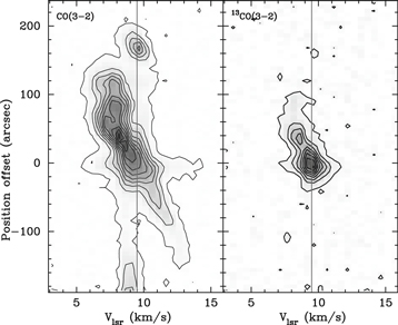
Figure 6. Position–velocity plots of CO(3–2) and 13CO(3–2) at p.a. = 0°, i.e., approximately at the symmetry axis of the blueshifted outflow. As one can see, the outflow is well separated in velocity from the R Mon molecular cloud, except at vicinity of R Mon. The position–velocity plots are plotted in gray scale overlaid with contours. The contours start in both cases at ∼3 sigma. For CO(3–2) we plot ten contours between 3σ and maximum intensity, while we only plot eight contours for 13CO(3–2). The redshifted outflow is not seen in 13CO(3–2), except in the immediate vicinity of R Mon.
Download figure:
Standard image High-resolution imageTo the south of R Mon the outflow is far less pronounced and redshifted, almost certainly because the molecular cloud is rather diffuse. Even though we see the cloud in CO(3–2) and dust emission (Figure 2), it is not detected in 13CO(3–2). This shows that the molecular cloud south of R Mon is mostly low column density. Hence there is very little gas for the outflow to interact with. The redshifted outflow stops ∼120'' south of R Mon. It appears more wide-angled, and more eastward than the blueshifted flow. The p.a. for the red outflow is ∼168°, while the blueshifted outflow is close to 0°.
3.2.2. Outflow Properties
The two-component Gaussian fits (Table 3) at the position of R Mon give a CO(3–2)/13CO(3–2) ratio = 1.86, which indicates that 12CO is completely optically thick. Even 13CO is optically thick with an optical depth of 1.7. Since we know the excitation temperature of the outflow, 77 K, from the analysis of Herschel SPIRE and PACS CO spectra (Jiménez-Donaire et al. 2017), we get a beam filling factor of CO(3–2) of 0.02, suggesting an envelope size of ≲25, because there is also some faint high-velocity emission outside the R Mon envelope. This agrees reasonably well with the CO(1–0) and CO(2–1) PdBI observations, which show CO(2–1) line wings brighter than 20 K for a beam size 19 × 09.
We derive the physical properties of the blueshifted outflow by integrating over narrow velocity intervals (0.5 or 1 km s−1) in both 12CO and 13CO. To determine the mass we adopt Tex = 77 K and a CO/H2 ratio of 10−4. At velocities close to the systemic velocity of the cloud, i.e., 1.3 km s−1 from the cloud center, the outflow is optically thick in CO. Therefore we used 13CO instead and adopted an isotope ratio 12CO/13CO = 50. At slightly higher velocities, 1.8 km s−1, 12CO is more extended than 13CO, but still optically thick, τ ∼ 2.1. Here we instead apply an opacity correction to the integrated 12CO intensity. At higher velocities 12CO is optically thin. The total mass in the blueshifted outflow is ∼0.56  , which is quite substantial. The inclination corrected momentum, P, and momentum flux, FCO, however, are rather low; P = 0.88
  km s−1, FCO = 0.08 × 10⁻⁵
  km s−1 yr−1. This is partly because the CO outflow has only moderate velocities, but more importantly, because most of the energy resides in the high-velocity optical jet.
The mass in the redshifted outflow is quite small, ∼0.12  . This is consistent with the low density in the cloud south of R Mon, which results in most of the outflowing gas escaping the cloud. The molecular gas therefore becomes too diffuse, and hence undetectable. The outflow velocities in the redshifted are similar to the blueshifted outflow. Assuming that the outflow momenta are the same in both the red- and the blueshifted outflow, we find that most of the redshifted outflow is invisible in CO.
The dynamical timescale, td, is difficult to estimate. Here we use the measured outflow velocity, 6 km s−1, the length of the outflow 0.62 pc, and an outflow inclination of 20° ± 10° (Close et al. 1997). With these parameters we derive td =  × 105 yr for the blue outflow. This is clearly an upper limit, since we know that the outflow extends well past the cloud surrounding R Mon, all the way to the Herbig–Haro cluster HH 39, 1.7 pc from R Mon. However, we do not know how fast the outflow moves, once it has cleared the cloud. We get a lower limit to the dynamical time by looking at the speed of the HH 39 condensations, which are moving away from R Mon at approximately the full stellar wind velocity (Jones & Herbig 1982). If they have been traveling with the same speed for most of the time, Jones & Herbig (1982) find that it has been 5900 yr since they left the vicinity of R Mon. The true dynamical timescale of the R Mon outflow is somewhere between these two extremes; a value of (2–5) × 104 yr appears reasonable although it could be longer.
4. The Nature of R Mon
R Mon is heavily obscured with an extinction, AV = 13.1 mag, determined from the IR part of the spectrum (λ > 1.28 μm). The optical and near-IR spectrum of R Mon is dominated by emission lines and weak Balmer absorption lines. Analysis of the near-IR H emission line strengths indicates heavy obscuration and an extinction of Av = 13.1. In the optical, scattered light effectively lowers the extinction derived from the emission line ratios. Close et al. (1997) derived a reddening value of 3.6 mag, but clearly the actual reddening to R Mon must be substantially larger than this.
The absorption line spectrum of R Mon is similar to that of an A supergiant, but exhibits no Balmer jump (Herbig 1968). Alonso-Albi et al. (2018) attempted to determine the spectral type of R Mon by fitting model spectra to the H absorption lines. However, as their figures demonstrate, a model of a normal main sequence does not fit the observed lines, as they are clearly far broader. We have carried out an analysis of the H absorption lines seen in the X-shooter spectrum obtained by Fairlamb et al. (2015) and also find that a normal main-sequence model does not fit them. A low surface gravity model, similar to that of a supergiant, provides the closest match to the observed line profiles. Since R Mon is a pre-main-sequence star it is impossible for it to be a supergiant. Rather, we suggest that the stellar photosphere is completely obscured, and the observed optical and NIR spectra are dominated by scattered light arising from the accretion disk. Hence it is impossible to determine a spectral type for R Mon from the observed optical and NIR spectra.
However, the bolometric luminosity is easy to measure and even though it does not allow us to determine the spectral type of the star, it puts stringent constraints on the stellar luminosity.
4.1. Bolometric Luminosity
Previous estimates of the bolometric luminosity of R Mon (Harvey et al. 1979; Cohen et al. 1985; Natta et al. 1993) using ground-based near/mid-IR observations and FIR photometry from the Kuiper Airborne Observatory ranged from 700 to 860  . Now there are much more accurate near-, mid-, and far-IR photometry available both from ground-based observations (Close et al. 1997), as well as from satellite mission like the Midcourse Space Experiment (MSX), Spitzer (Audard et al. 2007), the Wide-field Infrared Survey Explorer (WISE), and the Herschel Space Observatory. We have therefore assembled reliable photometry from the literature and the PACS and SPIRE images analyzed in this paper, see Table 2 and Alonso-Albi et al. (2009) for additional flux densities. Integrating the SED from 0.5 μm band to 1100 μm gives a total bolometric luminosity of 860
  , almost completely dominated by the emission in the near- and mid-IR. The FIR (30 μm–1 mm) portion of the luminosity, 150
  , is less than 20% of the total bolometric luminosity. Even if we assume that some of the far-UV radiation escapes the accretion disk/envelope surrounding R Mon, and use the flux densities within an 80'' radius around R Mon, we get a total bolometric luminosity of 960
  , an increase of only 100
  . At least some of this "extra luminosity" must arise from dust being heated externally by the general interstellar radiation field. Since more than 30% of the bolometric luminosity could come from the accretion disk (Natta et al. 1993), we conclude that R Mon cannot be an early B star. It simply does not produce enough luminosity to be one. It must be a late B star or even an early A star.
4.2. The R Mon Accretion Disk and Envelope
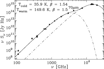
The mass of the accretion disk/envelope surrounding R Mon has been estimated to be in the range 0.1–0.24  (Natta et al. 1993; Mannings 1994; Sandell et al. 2011). Since there is now good photometry all the way into the FIR, we can do a better graybody fit than Sandell et al. (2011). We have accurate photometry from millimeter wavelengths to the FIR allowing us to simultaneously fit the cold outer envelope and warm inner core using an isothermal two-component model (see e.g., Sandell 2000; Howard et al. 2013). The least-squares fitting program allows us to put constraints on the dust temperature and size of the dust emitting regions, and fits simultaneously the dust temperature, source size, and the dust emissivity index, β. For the warm component we assume β = 1.5. In our fitting we use published millimeter and submillimeter photometry, FIR photometry from this paper (Table 2), and mid-IR photometry. We restrict the short wavelength end to 15 μm to avoid picking up hot dust from the inner accretion disk. We also omit mm-aperture synthesis data, because they filter out most of the emission from the extended envelope. The flux densities at millimeter wavelengths are corrected for free–free emission, as in Sandell et al. (2011). We find that the cold envelope has a dust emissity, β = 1.5, a temperature, Td = 36 K, and a radius of 25 ± 1.2. The temperature of the inner warm envelope is 150 K within a radius of 05. The fit is shown in Figure 7. Assuming standard Hildebrand dust opacity (κ250 μm = 0.1 cm2 g−1) and a gas-to-dust ratio of 100 (Hildebrand 1983), this corresponds to a total mass (gas + dust) of 0.34
  .
.
Figure 7. Two-component graybody fit to published millimeter and submillimeter photometry, FIR photometry (this paper), WISE, MSX, and Spitzer IRS data, see text. Since the x-axis is in frequency, we have plotted the PACS data as filled circles and the SPIRE data as filled squares. All other data points are shown as a filled triangle. The dash–dot lines show the warm and the cold component, with the solid line showing the total fit.
Download figure:
Standard image High-resolution image
5. Discussion
5.1. The R Mon Outflow
Our observations show that the blue outflow from R Mon has a p.a. of ∼0° at high velocities, suggesting that the R Mon accretion disk is essentially e–w, i.e., at a p.a of 90°. This is also supported by the high-angular resolution polarization imaging by Close et al. (1997), who found a "polarization disk" of low polarization at p.a. ∼90° (see their Figure 3). Furthermore, the imaging of the [S ii] jet with the Multi-Pupil Fiber Spectrograph on the 6 m telescope of the Special Astrophysical Observatory (Movsessian et al. 2002) shows that the jet has a p.a. of ∼0°, i.e., similar to what we see in CO.
The commonly assumed orientation for the R Mon outflow, p.a. = 350° comes from the assumption that HH 39 is on the symmetry axis of the outflow, which does not seem to be the case. However, based on this assumption, Fuente et al. (2006) assumed that the R Mon accretion would have a p.a. = 80°. It is therefore not surprising that they see blueshifted emission east of R Mon and redshifted emission to the west, giving the appearance of Keplerian rotation. However, as we have shown in Section 3.2.2, the outflow emission is optically thick in CO and even somewhat optically thick in 13CO in the R Mon envelope, therefore completely hiding any emission from the underlying accretion disk.
5.2. Comparison with Shock Models
Jiménez-Donaire et al. (2017), who analyzed Herschel PACS and SPIRE spectra, detected 26 CO lines, 6 OH lines, 4 H2O lines, [C i], [C ii], and strong [O i] 63 and 145 μm emission toward R Mon. The ratio [O i] 63 μm/145 μm is 9.9. Such a low ratio excludes a photon-dominated region (PDR) origin for [O i] because the ratio is typically 20 or higher (Keenan et al. 1994; Kaufman et al. 1999). The line ratio could be higher if the 63 μm line is self-absorbed, which is not very likely in a low-luminosity system like R Mon. There is overwhelming evidence that the line emission in R Mon is shock excited: strong, broad, and variable H i lines, and in particular the strong broad forbidden [S ii] and [O i] 6300 Å lines have to be shock excited. The observed [O i] line ratio suggests a gas density of ∼104 cm−3, if the main collision partner is atomic H (Nisini et al. 2015).
If we compare the observed PACS line intensities with the shock model predictions by Flower & Pineau des Forêts (2015), we find that the CO intensities agree well with a non-dissociative C-shock with shock velocities of 20–25 km s−1 and pre-shock gas densities of 104 cm−3. The observed OH intensities can still be explained with a C-shock although it requires higher shock velocities, 35 km s−1, and higher pre-shock densities, 104 cm−3. The observed OH lines can also be explained by a slow dissociative J-shock, 15 km s−1, and high pre-shock densities, 105. The observed [O i] intensities are far too high to be produced in a non-dissociative C-shock. They require a J-shock with a shock velocity 25–30 km s−1 and a pre-shock density of 105 cm−3. It therefore seems that in order to explain the observed line intensities the jet must power both J- and C-shocks.
5.3. Mass Loss and Accretion Rate
We obtain a mass-loss rate from the CO outflow of ∼(1–3) × 10−5  yr−1. This estimate is rather uncertain, because both the blue- and the redshifted outflow extends past the molecular cloud of R Mon, where it becomes too tenuous to be detected in CO. Furthermore, the dynamical timescale is very hard to estimate, see Section 3.2.2. We can get another estimate of the mass loss using the [O i] 63 μm PACS observations of R Mon (Jiménez-Donaire et al. 2017; Alonso-Albi et al. 2018). The [O i] luminosity is directly proportional to the mass-loss rate, if the jet velocity is high enough to produce a dissociative J-shock (Hollenbach 1985). From the previous paragraph we know that this is the case. We can therefore use the relationship

which is valid over a wide range of physical conditions. In the above expression  is the mass-loss rate in units of 10−5
  yr−1. Using the observed [O i] luminosity, 53.2 × 10⁻³
  (Jiménez-Donaire et al. 2017), we get a mass-loss rate of 0.5 10−5
  yr−1, i.e., similar to what we derived from CO.
The accretion rate is even more uncertain. Spectra of R Mon show no Balmer jump and there are no spectral features, which would allow us to determine an accretion rate. If we assume that the outflow is jet driven, which appears likely based on the observed properties of the outflow (Section 3.2.1), and further assume that the accretion rate is 0.1–0.3 times the outflow rate (Shu et al. 1994; Ferreira et al. 2006), we get (1–9) × 10−6  yr−1.
yr−1.
Mendigutía et al. (2011) were not able to derive an accurate accretion rate for R Mon, but estimate it to be in the range 3 × 10⁻³–7 × 10⁻⁶  yr−1. Our value is close to their low range and about ten times less than what Natta et al. (1993) estimated from theoretical modeling, 4 × 10⁻⁵
  yr−1.
yr−1.
Mendigutía et al. (2011) show that there is a clear correlation between accretion luminosity and Br γ luminosity for HAEBE stars, which appears to be somewhat flatter than for classical T Tauri stars. Although the empirical relationship derived by Mendigutíia et al. shows considerable scatter, it can at least provide us some estimates of the accretion luminosity. Br γ is much less affected by extinction and veiling than lines like Hα and [O i] 6300 Å, which all correlate well with accretion. There are several published observations of Br γ in the literature. Evans et al. (1987) only got an upper limit in 1985, <3 × 10⁻¹⁶ W m−2, while Carr (1990) detected it at approximately the same level in 1986, 3.6 × 10⁻¹⁶ W m−2. Nisini et al. (1995), who observed the line in 1991 December got 10.2 × 10⁻¹⁶ W m−2. This is about four times brighter than when it was observed by Carr (1990) indicating that there can be substantial variations in the accretion rate. If we extinction correct the observations for an AV = 13.1 mag and use the relationship between accretion luminosity and Br γ luminosity in Mendigutía et al. (2011) we get an accretion luminosity of 140–350  . This agrees quite well with what Natta et al. (1993) estimated from their theoretical modeling.
6. Summary and Conclusions
We have shown that R Mon is a young Herbig Be star, which drives a bipolar molecular outflow. The star is located in a cold (T = 20 K) filamentary cloud with a mass of ∼70  . The blueshifted outflow has excavated the molecular cloud north of R Mon, creating the reflection nebula NGC 2261 and filling it with high-velocity gas. At "high" velocities the orientation of the outflow is approximately n–s, i.e., p.a. ∼0°, which agrees with high-resolution imaging of the optical jet. Assuming that the accretion is orthogonal to the outflow, this implies that the accretion disk is e–w, P.A. ∼90°, which is also supported by high-resolution polarimetric imaging. R Mon is still surrounded by a massive envelope with a mass of ∼0.34
  . Toward R Mon the outflow is completely optically thick in CO(3–2), indicating that the size of the accretion envelope is ≲25. The outflow velocities are moderate, because the outflow is close to the plane of the sky, but the outflow is rather massive, ∼0.56
  in the blueshifted outflow lobe. The redshifted outflow lobe is ∼0.12
  . Both are underestimates, because the outflow has broken out of the molecular cloud, where the CO emission is no longer visible, see Section 3.2.2. The dynamical timescale is also very uncertain. ∼(2–5) × 104 yr, resulting in a mass-loss rate of ∼(1–3) ×10−5
  yr−1. Assuming the outflow is jet driven, this suggests an accretion rate of (1–6) × 10−6
  yr−1.We find that R Mon has bolometric luminosity of <1000
  , consistent with previous estimates. R Mon is still in an active accretion phase. Therefore a significant fraction of the observed luminosity is due to accretion. Hence R Mon cannot be a B0 star. It must be a late B star or it could even be an early A star.
Our observations are insensitive to the hot shocked gas (high J CO and [O i]), which dominates the energetics of the R Mon outflow. It would therefore be extremely useful to obtain velocity resolved spectra of these lines to study the shock characteristics in the region where the accretion shock dominates. The lines are bright enough to be easily observed with upGREAT or 4GREAT on the Stratospheric Observatory for Infrared Astronomy, SOFIA.
Footnotes
- *
Herschel is an ESA space observatory with science instruments provided by European-led Principal Investigator consortia and with important participation from NASA.
- 4
APEX, the Atacama Pathfinder Experiment is a collaboration between the Max-Planck-Institut für Radioastronomie, Onsala Space Observatory (OSO), and the European Southern Observatory (ESO).
- 5
CLASS is part of the Grenoble Image and Line Data Analysis Software (GILDAS), which is provided and actively developed by IRAM, and is available at http://www.iram.fr/IRAMFR/GILDAS.