


Abstract
The possibility of liquid water on present-day Mars has been debated for half a century. Melting is physically difficult under Martian environmental conditions, because with the total pressure of the atmosphere near the triple point pressure of water, evaporative cooling of ice is high near the melting point. Here, a suite of quantitative models is used to investigate whether melting of seasonal water frost can occur on present-day Mars. An updated and generalized parameterization is derived for the turbulent convective heat flux that results from the buoyancy of water vapor. A three-dimensional surface energy balance model is used to calculate surface temperatures; it includes terrain shadowing, self heating, and subsurface conduction. Protruding topography creates locations that experience a rapid transition from conditions where water frost accumulates to high solar energy input. Beyond the pole-facing side of a boulder, CO2 and  frost can accumulate seasonally, and once the Sun reemerges and the CO2 frost disappears, the water frost is heated to near melting temperature within one or two sols. Dust contained in the CO2 frost facilitates the formation of a protective sublimation lag. Temperatures within about 10 K of the melting point are reached within one or two sols after the end of water frost accumulation. For expected sublimation lag thicknesses, evaporative cooling is not significantly reduced. Overall, melting of pure water ice is not expected under present-day Mars conditions. However, at temperatures that are readily reached, seasonal water frost can melt on a salt-rich substrate. Hence, crocus melting behind boulders can lead to the formation of brines under present-day Mars conditions.
Export citation and abstract BibTeX RIS
1. Introduction
If liquid water exists on present-day Mars, it would have major implications for surface processes and astrobiology. Several young surface features have been attributed to the action of liquid water: gullies (Malin & Edgett 2000; Mellon & Phillips 2001; Christensen 2003; Heldmann et al. 2005; Williams et al. 2009), slope streaks (Ferris et al. 2002), and recurring slope lineae (McEwen et al. 2011), but subsequent observations rendered these interpretations less plausible (e.g., Schorghofer & King 2011; Diniega et al. 2013; Vincendon et al. 2019). A definite conclusion about whether liquid water is present anywhere on the surface of present-day Mars is lacking, and a satisfactory physical explanation of how it forms has remained elusive. If liquid water is present on the surface, it is transient and tied to small-scale topography (microclimates).
Under the physical conditions of present-day Mars, it is difficult to form or maintain liquid water (e.g., Ingersoll 1970; Kreslavsky & Head 2009; Forget et al. 2017). The partial pressure of  on Mars is presently about 0.15 Pa, about 4000 times lower than the vapor pressure at the triple point of
  (611 Pa), the minimum partial pressure necessary for pure liquid water. Hence, at and near melting, the saturated vapor above the condensed phase diffuses rapidly into the ambient atmosphere. Moreover, the total pressure of the atmosphere lies near the triple point pressure, so that ice near 0° C sublimates so rapidly that evaporative cooling becomes significant, and in fact exceeds the solar constant (Ingersoll 1970). Although the term "sublimation cooling" would be appropriate for ice, the more illustrative term "evaporative cooling" is used here. Figure 1 shows the phase diagrams of
  and CO2 to illustrate the relation between the triple point (611 Pa, 273.16 K), the frost point of
  (∼0.15 Pa, ∼200 K), and the total pressure of the atmosphere (∼520 Pa). In winter, CO2 from the atmosphere freezes out and the first day of spring without seasonal CO2 frost is, in the context of Mars, referred to as "crocus date." The total pressure of the atmosphere varies by about 30% throughout the year and ranges with elevation from 0.2–1 kPa at northern spring equinox (Smith & Zuber 1998). CO2 frost is seen on pole-facing slopes even at equatorial and mid-latitudes (Schorghofer & Edgett 2006; Carrozzo et al. 2009).

Figure 1. Phase diagrams of  and CO2 for pressure and temperature conditions on present-day Mars. The range of the horizontal temperature axis approximately corresponds to the range of surface temperatures reached on Mars. The range of total pressure is indicated by the shaded area. The typical partial pressure of
  in the Martian atmosphere is 0.13 Pa. Salts lower the triple point pressure and temperature.
Download figure:
Standard image High-resolution imageHere, one specific pathway for the formation of liquid water on present-day Mars is evaluated quantitatively: melting of seasonal water frost in rough terrain. In areas that are seasonally shadowed, water frost accumulates, and when the Sun rises again, temperature increases rapidly and may melt the frost. A rapid transition from cold to hot will involve little sublimation loss.
A number of relevant model studies have been previously conducted for melting of water ice on Mars. Farmer (1976) has written about the role of dust-covered ice or frost deposits as barrier to gaseous diffusion. The classic "dirty snow-pack model" by Clow (1987) closely corresponds to the pathway analyzed here, although in a two-dimensional setting. Williams et al. (2008, 2009) have reanalyzed the snow-pack model for sloped surfaces, with the snow as a leftover from a past climate period. Hecht (2002) has argued that radiative cooling is reduced in alcoves and has considered the influence of a restricted sky view on heat loss. Kossacki & Markiewicz (2004) modeled the full annual cycle of condensation and sublimation of atmospheric CO2 and  in gullies, accounting for the heat and mass transport in the soil. They found that water ice accumulated during winter can undergo transition to the liquid phase after complete sublimation of CO2 ice (in other words, crocus melting). However, they neglected buoyancy-driven convective heat loss.
Here, the possibility of melting of seasonal water frost is investigated based on a suite of quantitative improvements: (1) an updated and generalized quantification of the convective heat flux caused by the buoyancy of water vapor (Section 2); (2) a thermal model with three-dimensional surface energy balance (Sections 3); and (3) estimates of the role of a sublimation lag as diffusion barrier (Section 4).
2. Updated Formula for Rate of Free Convection
When the water vapor content of the atmosphere is a non-negligible fraction of the total atmosphere pressure, as will be the case near melting, there is a strong buoyancy force that leads to free convection and therefore strong evaporative cooling. At low partial pressure, sublimation is primarily by forced convection (wind-driven), but at high partial pressure it is by free convection (buoyancy-driven). Ingersoll (1970) quantified this effect, and here I update this equation based on parameterizations of turbulent flux from more recent literature. Table 1 summarizes variables frequently used in this section.
Table 1. Variables Frequently used in Section 2
| Gr | Grashof number |
| Nu | Nusselt number |
| Sh | Sherwood number |
| Ra | Rayleigh number |
| Pr = ν/κ | Prandtl number |
| Sc = ν/D | Schmidt number |
| C | a universal unitless constant |
| D | mass diffusivity (m2 s−1) |
| M1 | molecular weight of CO2 (44) |
| Mw | molecular weight of water (18) |

|
thermal conductivity (W m−1) |
| κ | thermal diffusivity (m2 s−1) |
| ν | kinematic viscosity (m2 s−1) |

|
dynamic viscosity (Pa s) |
| ρ | density (kg m−3) |
Download table as: ASCIITypeset image
2.1. Theoretical Form
By definition, the molecular flux (index m) and convective flux (index c) are related by


which defines the Nusselt number, Nu, and the Sherwood number, Sh. The molecular heat flux, Qm, is proportional to the temperature difference, ΔT, and the convective heat flux, Qc, can be written in the same form, only the coefficient of proportionality is no longer constant:


Here, L is a characteristic length scale, practically the dimension of the plate the laboratory experiment is conducted with. In some situations, L eventually cancels from the final expressions. For the mass fluxes,


where Dc is no longer constant. Here ρw is the density of water vapor, and the subscript w refers to H2O.
The governing equations for heat transfer without mass exchange and mass exchange without heat flow are, respectively,


where p is the partial pressure. The mechanical diffusivity, Dm, is that of one substance in another, D12 = D21 (binary diffusion), not that of a substance within itself, D11 (self diffusion). For free convection, the velocity  is in turn given by linear relations with T or p, respectively.
As the equations governing heat transport and mass transport are mathematically equivalent, both have the same solutions, even for turbulent flow. Both transport coefficients are given by the same function Φ (Jakob 1949),


The dimensionless numbers Gr, Pr, and Sc are similarity variables and will be defined below. In other words,  and
and  . Due to this similarity relation, measurements of
  for heat transfer can be used to determine Dc/Dm for mass transfer.
The function Φ has to be determined from laboratory measurements. For a large horizontal plate, Holman (1990) quotes the experiments by Fujii & Imura (1972) in water:

 is the Rayleigh number. Incropera et al. (2007) list
  for high Rayleigh number. Jakob (1949), which is the source of Ingersoll (1970), lists

based on laboratory measurements of heat transfer in air (Mull & Reiher 1930).
In the turbulent regime (at high Grashof number), the universal function Φ is in all these cases of the form

where N can be either  or
or  . Niemela et al. (2000) measured

in liquid helium and a specific container geometry. The small deviation from 1/3, if it applies to all geometries, would cause the length scale L to appear in the final result. From Equations (2), (10), and (13), we obtain the desired relation

The Grashof number is defined by

where g = 3.71 m s−2 is the specific surface gravity on Mars. The relative density difference,  , for temperature-driven buoyancy and humidity-driven buoyancy, respectively, is


where β is the coefficient for thermal expansion, which is 1/T for an ideal gas. In Equation (17), Δρ is the density difference between the warm and the cold air, whereas in (18) it is the density difference between the humid and the dry air.
The formula for the mass flux (6) then becomes

where the length scale L has now canceled, and  . The quantity

can be called "Grashof length scale" because it has units of length. One can also define  , although unlike C,
  is not a universal constant but depends on the Schmidt number for the specific gas composition. With these abbreviations,

2.2. Numerical Value of the Prefactor
Mills (2001), used in Dundas & Byrne (2010), directly provides

Hecht (2002) uses

The expression from Ingersoll (1970) is

Compared with Equation (19), this amounts to

which he based on Equation (12), which in turn can be rewritten as

It is unclear how the factor 0.17 was derived from this, as Pr and Sc of gases are close to one.
Table 2 summarizes the results for the universal prefactor, and in this work we adopt C = 0.14.
Table 2. Prefactor for Convective Flux from a Horizontal Plate
| Source |

|

|
C |
|---|---|---|---|
| Mass Transfer | Heat Transfer | ||
| Mull & Reiher (1930) a | ⋯ | (in air) | |
| Jakob (1949) | ⋯ | 0.068 in air | |
| Ingersoll (1970) | 0.17 on Mars | ⋯ | |
| Fujii & Imura (1972) a | ⋯ | (in water) | 0.13 |
| Holman (1990) | Quotes Fujii & Imura (1972) | 0.13 | |
| Mills (2001) | ⋯ | ⋯ | 0.14 |
| Hecht (2002) |

|
⋯ | 0.15 |
| Incropera et al. (2007) | ⋯ | x | 0.15 |
Note.
aOriginal measurements. Ingersoll (1970) is based on Jakob (1949), which fits data from Mull & Reiher (1930).Download table as: ASCIITypeset image
Now we consider the values of Sc, Dm, and ν, which are needed for the numerical evaluation of the equations. For an ideal gas  . For a hard-sphere model
  and
and  . Hecht (2002) uses a Schmidt number
  , where 0.78 is the Prandtl number for Mars atmospheric composition and at room temperature. Hence, expression (23) amounts to
  for Mars conditions and near melting.
Hudson et al. (2007) includes a comprehensive literature review for values of the vapor diffusivity. Based on this survey,  cm2 s−1 at standard temperature and pressure is a consensus value, which can then be scaled by pressure and temperature. For ideal gases, all three types of diffusivity (κ, Dm = D12, and ν) change with temperature and pressure proportionally to T3/2/p0.
The temperature dependence of dynamic viscosity η (Washburn 2003) is

For CO2, T0 = 273 K, η0 = 13.7 μPa s, and b = 240 K. The dynamic viscosity of a gas is nearly independent of pressure.
With these values for Dm and η, the Schmidt number for CO2 at 0° C comes out to about 0.47, similar to the value used by Hecht (2002). Both are low compared to theoretical expectation mentioned above. If we adopt a compromise value of  , then

for  in CO2 . This is lower than the 0.17 used by Ingersoll (1970).
Measured sublimation rates in a 7 mbar CO2 atmosphere (Sears & Moore 2005; Moore & Sears 2006) are consistent with Ingersoll's formula, but those authors did not provide any unitless constants, so a precise comparison of their laboratory measurements with the theoretical prefactor is not immediately available.
2.3. Modifications and Generalizations
Fujii & Imura (1972) measured heat loss from an inclined plane and found that for an inclination angle θ,  is to be replaced with
  . In other words, the convective flux is lower by a factor of
  compared to a horizontal plate. For a slope of 45°, this amounts to a factor of ∼0.9, so it is a small effect.
The partial pressure, pw, can never exceed the total pressure, p0, so evaporative cooling must compensate any value of heat input. In other words, in the limit  , the sublimation rate must diverge,
  , whereas in Equation (18)
  and Ec in (19) remains finite. For pw ≈ p0 the analogy between heat and mass transfer breaks down, because it assumes pw ≪ p0, so it is justified to change the asymptotic limit of Ec. For pw ≪ p0, Equation (18) reduces to
  , so it may as well be written as

which gives almost identical results for small pw, but diverges at pw = p0, as desired.
So far it was assumed that ice sublimates into a dry atmosphere. When sublimation is into an already humid atmosphere, the buoyancy forces are reduced. Near melting this effect is negligible, because, as described above, the humidity of the atmosphere is several orders of magnitude lower than that near the ice. Nevertheless, it is helpful to incorporate this into the equations so the transition to the case of stable ice, when the temperature is below the frost point, becomes continuous. Moreover, no buoyancy-driven convection occurs at low temperature, because wind-caused shear is higher, so the detailed quantitative form does not even matter. Denote the vapor density of the atmosphere as  . When the prefactor ρw in Equation (19) is changed to
  , the loss vanishes for
  , as desired.
In conclusion, the proposed new parameterization is
It updates the prefactor, diverges at pw = p0, and includes the inclination effect.
Figure 2 compares the parameterizations of Ingersoll (1970) and the updated version for a specific atmospheric pressure and a common set of material constants. The offset is due to the adjustment of the prefactor  from 0.17 to 0.12. The most significant difference is the divergence of the updated parameterization when the partial
  pressure approaches the total atmospheric pressure.

Figure 2. Updated parameterization for free turbulent convective heat flux driven by the buoyancy of water vapor in a 500 Pa CO2 atmosphere. The horizontal dashed line corresponds to the solar constant for Mars' semimajor axis. The vertical dashed line is the temperature for which the saturation vapor pressure equals the total pressure of 500 Pa. Both graphs are based on the same material constants.
Download figure:
Standard image High-resolution imageThe Grashof scale γ may be calculated as

3. Surface Energy Balance with Three-dimensional Topography
Terrain shadowing, restricted sky view, and infrared emissions from surfaces within field of view change the local energy balance. In particular, seasonal shadow can lead to the accumulation of CO2 and  frost, even at tropical and mid-latitudes, and the sudden rise of the Sun will lead to rapid heating of these frosts. To evaluate the thermal evolution, a numerical model is used that includes, in addition to direct insolation and subsurface conduction, also horizons and radiative energy exchange between surface elements.
3.1. Outline of Thermal Model
This section provides an overview of the model. Mathematical and implementation details are included in the User Guide that accompanies the online code archive (Schörghofer 2019). (The driving program used in this study is cratersQ_mars_full.f90, release 1.1.6.)
Shadowing by nearby topography (terrain shadowing) defines local horizons. Horizons for each surface element are determined with azimuth rays, with 2° azimuthal resolution, and the highest horizon in each direction is stored. For the purpose of horizon calculations, the topography is represented by triangular surface elements. The horizon elevations and view factors determined from these geometric calculations are stored in a file.
As the Sun moves through the sky, the model then simulates the time evolution of insolation (incoming solar radiation) and surface temperature, using the horizons and view factors as input. The surface energy balance is integrated over time at steps of 1/50 of a solar day (sol) for six Mars years. Surface temperature and insolation are updated at every time step.
The equation governing the energy balance on the surface is

where Qtotal is the total absorbed irradiance, k thermal conductivity, T temperature, z depth below surface,  emissivity, and σ the Stefan–Boltzmann constant. The equation of heat conduction is solved with a Crank–Nicolson scheme on a grid with spatially varying spacings.
The total radiative energy input is

where A is albedo. The flux Qdirect is determined from the decl. of the Sun, latitude, and hour angle. Due to topography, reflected sunlight (Qrefl) and thermal emission (QIR) from other surfaces also need to be added. The terms  and
and  are the long-wavelength and short-wavelength contributions from the atmosphere, based on a 0-dimensional model. F is the view factor of the sky.
The surface reemits radiation in all directions (Lambertian), but receives additional heat from surfaces in its field of view. These irradiances depend on view factors V,


where primed variables are evaluated at  and unprimed variables at (x, y). The integrals are over all surface elements with a direct line of view. This is the computationally most expensive component of the model calculations, and limits the investigation to small spatial domains.
3.2. Study Site Parameters
The model site is chosen at a latitude of 30° S. At the equator, seasonal effects would be small, and near the poles, peak temperatures would be low, so a mid-latitude location is ideal. A southern latitude is chosen, because the seasons are more extreme in the southern than in the northern hemisphere. Assumed are a surface albedo of 0.12 and an infrared emissivity of 0.98. The chosen albedo value is lower than the global average albedo of Mars, which favors higher peak temperature, but is realistic for many sites. The standard model run assumes a thermal inertia of 400 tiu (the thermal inertia unit, tiu = Jm−2 K−1 s−1/2).
The CO2 frost albedo is 0.65. The CO2 sublimation temperature is set to 145 K, as appropriate for the southern highlands. The albedo of the water frost is assumed to be the ambient albedo, as the frost is easily darkened by even a thin sublimation lag.
The three-dimensional surface energy calculations are initially carried out without any water frost. At locations of interest, the time series of absorbed energy is stored and the subsurface thermal model is rerun and reequilibrated with this energy as input to the surface energy balance. The presence of water frost is implied by subtracting the latent heat of its sublimation from the energy budget. Far from the melting point, that latent heat (the evaporative cooling) is negligible, but near the melting point it is significant and dependent on the total atmospheric pressure. The geoid-defined zero level of Mars Orbiter Laser Altimeter topography occurs at an average pressure of 520 Pa at Ls = 0° (Smith & Zuber 1998). The 610 Pa isobar lies, on average, 1600 m below that. The lowest-lying basin is the floor of Hellas basin, which lies about 7150 m below the topographic datum. There, the maximum annual pressure reaches 1.2 kPa (Haberle et al. 2001). Below, pressures of 500 Pa and 1 kPa will be considered for the evaluation of the evaporative cooling.
3.3. Results
Figure 3 shows model results for a bowl-shaped crater with a depth-to-diameter ratio of 1:5. Annual peak temperatures are above 273 K over the entire domain (on the ice-free surface). A small amount of CO2 frost forms seasonally on the pole-facing slope. Water frost accumulates continuously for up to hundreds of sols (the temperature continuously remains below the frost point temperature during this period). However, at least 95 sols pass between the end of continuous water frost accumulation and the first time 273 K is reached, so this geometry is not suitable for the melting of frost.

Figure 3. Thermal model results for a bowl-shaped crater at latitude 30° S and 400 tiu. North is up and equator-facing. Panel (b) shows the longest period of uninterrupted water frost accumulation. For comparison, the Mars year has 669 sols. Panel (d) shows the time between the end of continuous water frost accumulation and the first time the ice-free surface reaches 273 K.
Download figure:
Standard image High-resolution imageFor a boulder, here idealized as a half-sphere that sticks out from the surface (Figure 4), the situation is far more favorable. Beyond the southern (poleward) end of the boulder, water frost continuously accumulates for even longer periods, decimeters of CO2 frost accumulate, and peak temperatures are well above the melting point. Figure 5 shows the time dependence of a location behind the boulder, compared to that of the flat unobstructed surface. The third pixel from the edge was chosen, to avoid any potential corner artifacts. The location is seasonally shadowed around the winter solstice. After the Sun rises again the CO2 mass soon begins to shrink. After the crocus date, the surface temperature rapidly increases, and within 1 1/4 sols it reaches the melting point—when evaporative cooling is not considered. In other words, the diurnal maximum temperature goes from 145 to 273 K in such a short time.
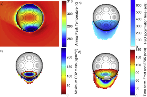
Figure 4. Thermal model results for a boulder at latitude 30° S and 400 tiu. The height-to-diameter ratio is 1:2. North is up and equator-facing.
Download figure:
Standard image High-resolution image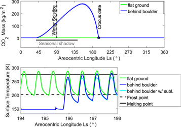
Figure 5. Time dependence of CO2 mass and surface temperature behind the pole-facing slope of the boulder. The location is marked with a white cross in Figure 4. The total atmospheric pressure is 1000 Pa.
Download figure:
Standard image High-resolution imageThese calculations show that even CO2 frost can be expected at locations that subsequently reach temperatures above 273 K, consistent with the results by Kossacki & Markiewicz (2004), and this prolongs the duration of  frost. Once the Sun rises, the CO2 ice begins to sublimate, but the CO2 –
 ice composite cannot warm until all of the CO2 ice has disappeared. By this time, the insolation will be even more intense. After this point, the
  frost, none of which has yet been lost to the atmosphere, will experience rapid warming.
The peak surface temperatures behind the boulder are no higher than for an unobstructed surface (Figure 5), so the topography provides no energetic advantage during peak periods. The significant role of the topography is to cast a seasonal shadow. The depression (Figure 3) and the protruding topography (Figure 4) both cause seasonal CO2 accumulation, but only for the protruding topography (the boulder) is there a rapid transition from cold conditions to low solar incidence angles ("high Sun").
With evaporative cooling, the surface does not reach the melting point (Figure 5). In this model calculation, 1000 Pa and pure ice (no lag deposit) are assumed. The albedo of the  frost is assumed to be only 0.12, as reasonable if darkened by a lag. On Earth, the albedo of old snow is typically 0.4. But a lag deposit only a few particles thick can darken the surface tremendously. On the first full sol after the crocus date, the temperature rises to 256 K and 0.1 kg m−2 of frost are lost until it first reaches this temperature. This is the equivalent of a 100 μm thick layer of water. The next day, the peak temperature is 260 K and at this point 0.5 kg m−2 of frost have been cumulatively lost. The evaporative cooling is too strong to allow 273 K to be reached. Melting temperature would be reached, if the loss rate were artificially reduced by a factor of 20.
For an atmospheric pressure of 500 Pa, the values are similar. The peak temperature on the first full sol is 254 K and 0.15 kg m−2 of frost (0.15 mm thickness) were lost. On the next sol, the peak temperature is 257 K.
The Viking 2 Lander observed almost continuous early frost 10–20 μm thick, and later patchy frost probably 100–200 μm thick (Svitek & Murray 1990). More frost may accumulate in well-shadowed alcoves. Hence, the mass lost within a sol or two after the crocus date is within the amount that can be expected to be present.
Thermal model calculations were carried out not only for a thermal inertia of 400 tiu, but also 200 and 1000 tiu. The different thermal inertias change the crocus date, but the peak temperatures are about the same and melting temperatures were not reached.
4. The Overlying Layer
4.1. Diffusion Barrier
A layer of dry material overlying the ice acts as a diffusion barrier and reduces mass loss and evaporative cooling. Such a layer could form as a sublimation lag if dust is included during deposition. The dust content of terrestrial snow is rather low, but deposition rates on Mars are much lower, and therefore the relative dust content could be much higher. If the overlying layer is thin enough, it dampens the diurnal temperature amplitude only slightly so that the underlying ice experiences similar peak temperatures as the surface. Next, we quantitatively evaluate the reduction in sublimation loss due to an overlying dust layer.
When the partial pressure of the water vapor is much lower than the total pressure, the flux through the porous layer is in the form of molecular diffusion,

where Dℓ is the vapor diffusivity of the porous layer. The water vapor density on the surface is ρs, while ρw is the vapor density at the buried ice surface and equals the saturation vapor density. The approximation, which amounts to a steady-state model, should be valid for a thin layer subjected to nearly periodic temperature cycles.
With advection, there is a pressure difference across the layer, and the flux becomes (Hudson et al. 2007)

where c = ρv/ρ0. This relation is no longer useful at c = 1, but it establishes that for high vapor content, advection enhances the flow, and it has the desired property that the flux diverges for ρv = ρ0. The pressure difference can at most be the weight of the overlying layer, which is small, e.g., 1300 kg m−3 × 3.7 m s−2 × 0.01 m = 48 Pa for a 1 cm thick layer. Hence, the partial  pressure still cannot surpass the atmospheric pressure by a significant amount. A practical approximation for the advection correction that retains the qualitative behavior is to replace (36) with

The flux from the surface to the atmosphere is analogous to (21)

Eliminating ρs from (38) to (39) yields

Hence, the diffusion barrier becomes significant when

When the pore sizes are larger than the mean-free path in the atmosphere, Dℓ = Dm, where is the porosity of the dry layer. The mean-free path in the Martian atmosphere is about 10 μm (Hudson et al. 2007). The cross-section for molecular diffusion is restricted by a factor of relative to the entire cross-sectional area available for molecular diffusion in the atmosphere. In this case, the diffusion barrier becomes significant when ζ ≳ γ/C'. The porosity is ≈ 0.42 for a randomly packed granular medium, and  , so in this case ζ ≳ 3.5γ.
For micron-sized particles (commonly referred to as dust-sized) the pore sizes are smaller than the mean-free path, and Dℓ/Dm can take on smaller values. For example, for a pore size of 1 μm, ten times less than the mean-free path in the atmosphere, the threshold would be ζ ≳ 0.4γ. Micron-sized particles are known to be suspended in the Martian atmosphere. In conclusion, for the dust layer to be a significant barrier to vapor diffusion, its thickness needs to be on the order of the Grashof length scale γ.
Figure 6 shows values for γ according to Equation (31) with a linear vertical axis. At 260 K, γ is about one centimeter. For an overlying layer to significantly reduce the mass flux, and therefore, evaporative cooling, it would have to be nearly that thick. Dust is incorporated in frost and snow, but to form a sublimation lag, a far thicker layer of ice must first be lost. If the dust content is 1%, then about 10 cm of ice need to be lost to leave behind a 1 mm thick layer of dust. A protective dust layer could also originate from a dust storm.

Figure 6. Grashof length scale γ for Mars conditions.
Download figure:
Standard image High-resolution imageSeasonal CO2 frost is easily decimeters thick. If enough dust is incorporated into the CO2 ice during accumulation, a dust layer will build up as the CO2 sublimates back into the atmosphere, leaving behind water frost and the dust.
4.2. Peak Temperatures with and without Sublimation Lag
A typical diurnal thermal skin depth for dust on Mars is 4 cm, so a layer a few mm thick will not significantly dampen the temperature amplitude.
The thermal model calculations in Section 3 demonstrated that sudden transitions from frost-accumulating conditions to near-melting conditions occur, but ultimately there is not enough energy available to compensate for the evaporative cooling. Here, we focus on the energetics, with and without a protective layer, using an idealized energy input.
An idealized form for the absorbed solar flux is

where A is albedo, S0 = 1360 W m−2 the solar constant, R the distance from the Sun in au, and i is the incidence angle, assumed to change linearly with time. The factor of 0.96 represents net absorption in the Martian atmosphere. This approximation represents the Sun rising and setting at an equatorial location at equinox. The equilibrium surface temperature T is calculated by numerically solving the nonlinear equation  , where LH2O is the latent heat of sublimation and J the sublimation rate (40).
Figure 7 shows the surface temperature and the time-integrated loss over a quarter of a sol (from morning until noon). At an atmospheric pressure of 500 Pa, below the triple point, 273 K cannot be reached. For exposed ice, the surface temperature reaches 264 K and about 1.2 kg m−2 ice, if available, is lost during this quarter sol. With 2 mm of very fine sublimation lag, these values remain almost the same (267 K and 1.1 kg m−2). For an atmospheric pressure of 1 kPa and without overlying layer, the peak temperature is 269 K and the loss 1.1 kg m−2 by noon. For an atmospheric pressure of 1 kPa and a 3 mm thick layer of micron-sized particles, 273 K is reached and the ice loss until this point of time is about 0.5 kg m−2 (about 500 μm). This last result is for rather favorable conditions: solar energy input at the equator, at perihelion, equilibrium temperature (zero thermal inertia), a high pressure of 1000 Pa, and a thick lag consisting of micron-sized particles. Realistically, this ideal combination cannot be expected for any place on Mars, so the conclusion is that crocus melting of pure ice does not occur on present-day Mars.

Figure 7. Ice loss from morning until noon with idealized solar energy input, on a horizontal unobstructed surface. Solar energy input corresponds to the equator at perihelion, an albedo of 0.15, and an infrared emissivity of 0.98. (a) Equilibrium surface temperature as a function of local time on Mars. The atmospheric pressure is p0, and ζ is the thickness of an overlying dust layer of micron-sized dust particles ( ), so that ζ = 0 corresponds to exposed ice. (b) Ice loss as a function of local time. A layer of water 1 mm thick has a column density of 1 kg m−2.
Download figure:
Standard image High-resolution image
For a frost albedo of 0.4 instead of 0.15, the noontime temperatures are lower by about 5 K in all four cases. Having enough refractory material to darken the surface contributes notably to the peak temperature.
These results show: (1) the consequences of evaporative cooling are severe. For all but the most favorable conditions, the melting point is not reached. (2) A sublimation lag of a few mm reduces the sublimation loss only slightly. At 500 Pa, a 2 mm sublimation lag of micron-size particles increased the peak temperature only by 3 K. (3) Peak temperatures within about 10 K of the melting point within two sols of the crocus date are realistic. The full thermal model calculations with exposed (but darkened) ice resulted in peak temperatures of 254–260 K within the first two sols after the crocus date. For the energetically more favorable situation considered in this section, exposed ice reaches 264–269 K at noon. For realistic energetics and a thin sublimation lag, 263 K is a realistic peak temperature. (4) Since the energetics considered in this section is close to optimal for the present orbit (at perihelion, Sun rising to zenith, dark frost), changes in latitude and axis tilt will not suffice to cause crocus melting. The three-dimensional thermal model calculations demonstrated that a sudden transition from frost-accumulating conditions to hot conditions can occur. They were carried out for only one site, but other site locations or site parameters would still not have a higher maximum energy input than was assumed for the idealized model.
5. Discussion
The parameterization of the convective mass flux is based on indirect laboratory measurements, and carries uncertainty with it. The regime where ρw is comparable to ρ0 has the least footing in quantitative theory. Moreover, more confined geometries might reduce this flux. An additional modification applies for sources of small spatial extent, although the flux would in this case arguable be increased. As mentioned in an example above, the heat flux would have to be reduced by an order of magnitude, compared to the current estimate, to allow for crocus melting of pure ice behind boulders under common Mars conditions.
Through the crocus melting pathway, temperatures can readily come within about 10 K of the melting point of pure ice. Salts are commonplace on Mars, and seasonal frost could melt on a salt-containing substrate to form a brine (Brass 1980; Hecht et al. 2009). They have a range of eutectic temperatures, and the temperatures produced through crocus melting behind boulders would suffice, even at atmospheric pressures below that of the triple point of pure water. The process will repeat periodically until the salt is depleted. Overall, it is realistic that seasonal water frost melts on salt-rich ground for a few hours per Mars year. Since the seasonal frost layer is very thin, the total volume of brine produced is small.
Crocus melting of pure water frost could become commonplace if the atmospheric pressure was significantly higher during a past climate period. The south polar perennial residual CO2 ice cap is expected to disappear over timescales of the precession cycle (51 ka), but that CO2 ice layer is estimated to add only ∼3% to the atmospheric pressure (Titus et al. 2017). Larger reservoirs of CO2 ice may be sequestered deeper in the South Polar Layered Deposit or adsorbed in the regolith (Titus et al. 2017), and these could be released further in the past. (It is not known whether this has occurred over the last 4 Ma).
6. Conclusions
The possibility of melting of seasonal water frost is investigated based on (1) an updated quantification of the convective heat flux caused by the buoyancy of water vapor, Equation (30); (2) detailed thermal model calculations with three-dimensional surface energy balance (including subsurface conduction, terrain shadowing, and self heating); and (3) estimates of the role of a sublimation lag as diffusion barrier.
The thermal model calculations demonstrate that protruding topography in the mid-latitudes can cause a sudden transition from frost accumulation to high diurnal maximum temperature. Even seasonal CO2 frost is expected to form, and the rapid temperature rise occurs on and following the crocus date. The CO2 ice prolongs the presence of water frost, by absorbing the incoming energy through its latent heat and also facilitates formation of a sublimation lag, sourced from the dust included in the ice volume. Without evaporative cooling, 273 K can be reached within 1/4 or 1 1/4 sols after the end of water frost accumulation.
Evaporative cooling prevents temperatures from rising to 273 K, even at an atmospheric pressure as high as 1000 Pa and even with a sublimation lag of several mm of dust (although both combined can be sufficient). However, dark water frost can reach peak temperatures within about 10 K of the melting point, and the loss of ice experienced during the warming phase is no larger than the amount of seasonal water frost that can be expected to be present. These temperatures may be high enough for saline water to form annually in spring.
Thanks to Misha Kreslavsky for introducing me to the term "crocus melting" and to Paul Hayne, Joe Levy, and Mathieu Vincendon for insightful discussions. This material is based upon work supported by the National Aeronautics and Space Administration under grant No. NNX17AG70G issued through the Habitable Worlds Program.