


Abstract
We develop and implement a model to analyze the internal kinematics of galaxy clusters that may contain subpopulations of galaxies that do not independently trace the cluster potential. The model allows for substructures within the cluster environment and disentangles cluster members from contaminating foreground and background galaxies. We estimate the cluster velocity dispersion and/or mass while marginalizing over uncertainties in all of the above complexities. Using mock observations from the MultiDark simulation, we compare the true substructures from the simulation with the substructures identified by our model, showing that 50% of the identified substructures have at least 79% of its members are also members of the same true substructure, which is on par with other substructure identification algorithms. Furthermore, we show a ∼35% decrease in scatter in the inferred velocity dispersion versus true cluster mass relationship when comparing a model that allows three substructures to a model that assumes no substructure. In a first application to our published data for A267, we identify up to four distinct galaxy subpopulations. We use these results to explore the sensitivity of inferred cluster properties to the treatment of substructure. Compared to a model that assumes no substructure, our substructure model reduces the dynamical mass of A267 by ∼22% and shifts the cluster mean velocity by ∼100 km s−1, approximately doubling the offset with respect to the velocity of A267's brightest cluster galaxy. Embedding the spherical Jeans equation within this framework, we infer for A267 a halo mass M200 = (7.0 ± 1.3) × 1014 M⊙ h−1 and concentration  , consistent with the mass–concentration relation found in cosmological simulations.
Export citation and abstract BibTeX RIS
1. Introduction
Galaxy clusters are the most massive gravitationally bound and relaxed structures in the universe, thereby representing important laboratories for observational cosmology (Rines et al. 2003, 2013; Voit 2005; Jones et al. 2009; Vikhlinin et al. 2009; Geller et al. 2013; Sohn et al. 2017). Due to their high density of galaxies, they are also ideal for studying galaxy interactions and the effect these interactions have on the galaxy population. Galaxy clusters are studied in a multitude of ways, from gravitational lensing, both weak and strong (e.g., Kneib 2008; Postman et al. 2012; Applegate et al. 2014; Barreira et al. 2015; Gonzalez et al. 2015, and references therein), to X-ray temperature measurements of hot intracluster gas (Guennou et al. 2014; Moffat & Rahvar 2014; Girardi et al. 2016; Rabitz et al. 2017), to Sunyaev–Zeldovich effects (Sunyaev & Zeldovich 1970; Churazov et al. 2015), to spectroscopic velocity measurements of cluster members (e.g., Rines et al. 2003, 2016; Geller et al. 2014; Stock et al. 2015; Biviano et al. 2016; Tasca et al. 2017, and references therein). All of these methods can provide mass estimates, thus constraining the high-mass end of the halo mass function, thereby constraining cosmological parameters such as the amplitude of the power spectrum or the evolution of dark matter and dark energy density parameters.
When calculating cluster masses using the velocities of cluster members, it is common to assume that the cluster is a relaxed system with a gravitational potential and kinematics that satisfy the viral theorem. However, such assumptions neglect recent galaxy accretion that could alter the distribution of galaxies in phase space (Regos & Geller 1989; van Haarlem et al. 1993; Diaferio & Geller 1997; Rines et al. 2003). Additionally, even in systems that appear relaxed, these mergers can generate residual substructure within the cluster environment such that individual galaxies are not necessarily independent tracers of the gravitational potential (Dressler & Shectman 1988; Biviano et al. 2002; Girardi et al. 2015). These factors have the potential to impact dynamical mass measurements, leading to systematic errors that will then propagate into cosmological inferences.
Recent efforts have been made to identify substructure within galaxy clusters. There are many 3D, 2D, and 1D tests for substructure that have been developed in the past few decades (Dressler & Shectman 1988; West et al. 1988; West & Bothun 1990; Coziol et al. 2009; Hou et al. 2009). Pinkney et al. (1996) compared and discussed the validity of some of the earlier tests, while others have applied them to Sloan Digital Sky Survey (SDSS) clusters (Einasto et al. 2012). Recent efforts in substructure analysis have focused on identifying subpopulations based on galaxy morphological types (e.g., Biviano et al. 2002; Barrena et al. 2007; Chon et al. 2012; Girardi et al. 2015). Accounting for such substructure when measuring dynamical masses is vital in achieving accurate estimates. For example, Old et al. (2018) have shown that almost all dynamical mass estimators overestimate cluster masses for clusters with significant dynamical substructure compared to estimates for clusters without substructure.
Furthermore, the identification and proper modeling of substructure may be important for distinguishing among competing models for the nature of dark matter. For example, under the standard cold dark matter (CDM) paradigm, dense "cusps" form at the centers of dark matter halos (Dubinski & Carlberg 1991; Navarro et al. 1996, 1997). In galaxy cluster halos, CDM cusps will tend to bind the brightest cluster galaxy (BCG) near the halo center. However, recent simulations suggest that if the dark matter undergoes significant self-interactions, the subsequent unbinding of central cusps (particularly in response to major mergers) would allow BCGs to "wobble" about the cluster center (Harvey et al. 2017; Kim et al. 2017). Such wobbles could be detected as offsets between clusters and their BCGs in the projected phase space. Substructure can affect the detection of such offsets, as the elements within a given substructure do not independently sample a phase space that is representative of the cluster itself.
Clearly, substructure can affect inferences about the internal dynamics of galaxy clusters. Here we devise a framework that can account for both affects simultaneously. This allows us to study the impacts of both phenomena on cluster mass estimates and to marginalize over uncertainties in rotation and substructure. In this paper we apply this model to our own published spectroscopic observations of A267 (Tucker et al. 2017), combined with measurements from the redshift catalog HectoSpec (Rines et al. 2013) to achieve a large sample. We summarize these data sets in Section 4.1. In Section 2 we describe the dynamical model, and we then apply the model to A267 assuming a uniform velocity dispersion (Section 4.3) and a dark matter halo model (Section 4.4). Throughout the paper we use H0 = 100 h−1 km s−1 Mpc−1 and mass density Ωm = 0.3.
2. Galaxy Cluster Mixture Model
In this section we describe the mixture model for galaxy cluster substructure analysis.
We model the observed distribution of galaxy positions and redshifts as a random sample from several distinct galaxy populations. We define the populations as the main cluster population, a set of subpopulations of galaxies within the cluster, and a contamination population including both foreground and background galaxies. Because spectroscopic observations are used as follow-up to already-identified clusters with good photometry, the model incorporates into the likelihood function the sky positions from a full photometric catalog, as well as spectroscopic line-of-sight velocity measurements of a subset of these galaxies. Therefore, we define the likelihood function that, given a set of model parameters  , describes the observed position and velocity distribution as

where  is the likelihood function associated with the photometric data set and
  is associated with the spectroscopic data set.
We model the discrete photometric sample of galaxies as being drawn independently from an underlying surface brightness profile  . Therefore, the likelihood for the observed photometric sample is (Richardson et al. 2011)

where  is the field of view (FOV),
  is the surface brightness profile, Ngal is the number of galaxies observed in the photometric data set, and
  is the position on the sky of each galaxy. The constant of proportionality here does not depend on the model. For a multipopulation model, the surface brightness profile is the sum of the profiles for each individual population:
where Np is the number of populations in the model. For the purposes of this paper we assume that all profiles (main cluster halo and substructures) are dark matter dominated and therefore follow a Navarro–Frenk–White (NFW) profile (Navarro et al. 1996):
where νs and rs are the scale density and radius of an NFW profile, respectively. Equation (4) simply projects the 3D light profile νNFW onto the plane of the sky, yielding the 2D light profile INFW. Luckily, this projection is analytic for an NFW profile and is given by
where x = r/rs (Bartelmann 1996).
The spectroscopic likelihood function used to describe the velocity distribution is

where Nspec is the number of galaxies from the photometric catalog with spectroscopic derived line-of-sight velocities vi and  is the probability distribution of measured line-of-sight velocity vi, given position
  , and model parameters
  . We can then marginalize this distribution over the populations and invoke Bayes's rule to write
The first term in the numerator is simply the number fraction of galaxies within that population:  . The second term in the numerator,
  , is the probability for a galaxy at position
  given the population M and the model
  , which is directly proportional to the surface brightness profile of the population:
  . The denominator we can again marginalize over the populations so that
  . And so we can rewrite Equation (7) as
The final probability distribution in Equation (8) describes the velocity distribution for a given population M and position  . The modeling framework is flexible in the sense that any choice of a velocity distribution function can be used here. Although it is not the most physically motivated model, we use a Gaussian velocity distribution similar to Mamon et al. (2013) because it is easy to implement numerically and is a fairly good approximation for the observed profile of galaxy clusters:
where δi is the measurement uncertainty in line-of-sight velocity vi,  is the projected velocity dispersion profile of the Mth population evaluated at the sky position of each galaxy
  , and
, and  is the average velocity of the Mth population. Once again the modeling framework is flexible to a variety of choices of projected velocity dispersion profile. In Sections 3 and 4.3, we apply a uniform velocity dispersion
  for both the main cluster halo and all subpopulations, whereas in Section 4.4 we assume that the velocity dispersion of the main cluster halo follows a dark matter halo such that it is radial symmetric
  and can be evaluated using a Jeans analysis.
For real observations from galaxy redshift catalogs, the contamination population of galaxies is typically dominated by foreground and background clusters that happen to lie along the line of sight to the cluster of interest. For this reason, extra care must be taken when choosing a physically motivated contamination model. We discuss the specific choices made for contamination models in Sections 3.3 and 4.2 below.
For every model  , we can evaluate the probability that each galaxy is a member of the various populations. Given a galaxy's velocity vi and position
  , the probability that it is a member of population M is
In the following sections we will use "probability of membership to the cluster" to refer to the probability that an individual galaxy belongs to either the main population or any subpopulation, and we define this membership probability as  .
.
In order to fit this model, we use the nested sampling algorithm MultiNest (Feroz et al. 2009), which simultaneously calculates the Bayesian evidence, used for model selection, and generates random samples from the posterior probability distribution. We will use the Bayesian evidence as a metric to select the optimal number of subpopulations for a given data set.
3. Tests with Mock Observations from Simulations
The main goal of this modeling framework is to produce more accurate estimates of cluster masses by accounting for substructure of the cluster. Therefore, as a first test of this modeling framework, we use mock galaxy cluster redshift catalogs produced from the MultiDark Planck 2 N-body simulation (MDPL2; Klypin et al. 2016).
3.1. The MultiDark Simulation
We conduct this analysis with mock observations generated from a publicly available snapshot from MDPL2 simulation.6 MDPL2 is an N-body dark-matter-only simulation with 38403 particles in a box of length 1 Gpc h−1 and a mass resolution of 1.51 × 10⁹ M⊙ h−1. The simulation was executed using L-GADGET-2 (Springel 2005) and uses a Planck ΛCDM cosmology (Planck Collaboration et al. 2014): ΩΛ = 0.693, Ωm = 0.307, h = 0.678, n = 0.96, σ8 = 0.8828.
Halos and subhalos were identified from simulation data using the ROCKSTAR halo finder (Behroozi et al. 2013), which performed a clustering algorithm in the 6D phase space (three positions and three velocities) of dark matter particles. Subhalos were then populated by galaxies using the galaxy assignment procedure UniverseMachine (Behroozi et al. 2019). Unlike other galaxy assignment procedures, UniverseMachine is able to track the gravitational evolution of each galaxy's subhalo even below the resolution limit of ROCKSTAR, thus increasing the total number of simulated galaxies. The resulting catalogs provide information on the cluster mass and size, as well as 6D phase-space information on each galaxy: comoving position and proper velocity information.
3.2. Mock Observations
Mock observations are generated from these galaxy cluster catalogs using the prescription described in detail in the Appendix of Ho et al. (2019). The general procedure is as follows. First, a large cylindrical cut about the center of each cluster is made in projected phase space with radius of 10 Mpc h−1 and length ±6 × 10³ km s−1 oriented along the line of sight. This large cut will include the infall region of the cluster and include contamination galaxies that could fall along the line of sight to the cluster. Each galaxy that falls within this cylinder (and has a mass at accretion  h−1) will be projected along the line of sight, thus producing a catalog of simulated observations of sky positions and line-of-sight velocities. For each cluster, we follow this procedure for three separate orthogonal pointings, thus producing three mock observation catalogs for a given cluster, which (for statistical purposes) we treat as independent clusters.
We divide clusters into a low- and a high-mass sample. The low-mass sample has a mass range from  h−1 to 0.96 × 10¹⁴
  h−1 with a median 0.86 × 10¹⁴
  h−1, and the massive sample ranges from 0.63 × 10¹⁵
  h−1 to 2.04 × 10¹⁵
  h−1 with median 0.98 × 10¹⁵
  h−1. All mass values listed here and for the remainder of this section are M200c and defined as the mass enclosed by a spherical overdensity 200 times the critical density of the MDPL2 simulation, and these masses are calculated using all dark matter particles belonging to the cluster's ROCKSTAR halo that fall within the spherical overdensity. We used the z = 0.117 snapshot and placed the observer at z = 0. Furthermore, the mock observation generation does not include observational effects such as obstructions or lensing.
Figure 1 shows two sets of mock cluster observations. The top set is one of the low-mass clusters, while the bottom is a high-mass cluster. In total, our galaxy cluster sample includes 92 unique clusters from the simulation volume (half in the high-mass bin), projected along three orthogonal pointings, totaling 276 mock galaxy cluster redshift catalogs. For each redshift catalog, we use all sky positions of galaxies as our photometric data set, but we select a subset of these galaxies (80%) to produce the spectroscopic catalog that includes the line-of-sight velocities. We produce 10 random samplings of each galaxy cluster redshift catalog.
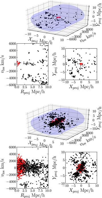
Figure 1. Two example mock observations of clusters produced from MDPL2. The top cluster is part of the low-mass sample, while the bottom is from the high-mass bin. The red points are galaxies that are members of the ROCKSTAR cluster halo.
Download figure:
Standard image High-resolution image3.3. Model Setup
For each mock cluster catalog we fit four multipopulation models with  . For each model we assume a uniform velocity dispersion for the main cluster halo and all substructures:
  . For the contamination model, we assume a uniform distribution of galaxies on the sky, as well as a uniform velocity distribution:
where Σ0 is a free parameter in the model, while vmax and vmin are set by the range of velocities in the data set. Therefore, each model in total includes two free parameters for the contamination model, five free parameters for the main halo, and six free parameters for each subpopulation. All free parameters, the chosen prior, and a description are listed in Table 1.
Table 1. Free Parameters and Priors for MultiDark Mock Observation Models
| Parameter | Prior | Description |
|---|---|---|
![${\mathrm{log}}_{10}\left[{{\rm{\Sigma }}}_{0}/{(\mathrm{Mpc}{h}^{-1})}^{-2}\right]$](https://content.cld.iop.org/journals/0004-637X/888/2/106/revision1/apjab609dieqn36.gif)
|
Uniform between −5 and 5 | Uniform contamination light profile |
| fcontam | Uniform between 0 and 1 | Number fraction of contamination galaxies |
![${\mathrm{log}}_{10}\left[{r}_{s,\mathrm{main}}/{R}_{\max }\right]$](https://content.cld.iop.org/journals/0004-637X/888/2/106/revision1/apjab609dieqn37.gif)
|
Uniform between −3 and 0 | NFW scale radius of main halo light profile |
![${\mathrm{log}}_{10}\left[{r}_{c,\mathrm{main}}/(\mathrm{Mpc}\ {h}^{-1})\right]$](https://content.cld.iop.org/journals/0004-637X/888/2/106/revision1/apjab609dieqn38.gif)
|
Uniform between −6 and −1 | Radial offset of center of main halo |

|
Uniform between 0 and 2π | Angular location of center of main halo |
| zmain | Uniform between 0.1 and 0.15 | Redshift of main halo 
|

|
Uniform between 0 and 3.5 | Velocity dispersion of main halo |
![${\mathrm{log}}_{10}\left[{r}_{s,\mathrm{sub},i}/{R}_{\max }\right]$](https://content.cld.iop.org/journals/0004-637X/888/2/106/revision1/apjab609dieqn42.gif)
|
Uniform between −3 and 0 | NFW scale radius of ith substructure light profile |
![${\mathrm{log}}_{10}\left[{r}_{c,\mathrm{sub},i}/{R}_{\max }\right]$](https://content.cld.iop.org/journals/0004-637X/888/2/106/revision1/apjab609dieqn43.gif)
|
Uniform between −3 and 0 | Radial offset of center of ith substructure |

|
Uniform between 0 and 2π | Angular location of center of ith substructure |

|
See Equation (12) | Velocity of ith substructure |

|
Uniform between 0 and 1 | Velocity dispersion of ith substructure |
| fi | Uniform between 0 and 1 | Number fraction hyperparameter |
Download table as: ASCIITypeset image
Most free parameters listed in Table 1 have uniform prior distributions; however, we use a nonuniform prior to determine the mean velocities of the substructures. This prior choice was made after considering two related issues with the modeling. First, we need to invoke an identifiability requirement so that the Bayesian sampling algorithm (MultiNest) can differentiate between the various populations; we do this by requiring the substructures to have decreasing velocity (i.e.,  ). If we were to implement this requirement using uniform priors with a maximum value specified by the i − 1 velocity, then the true prior distribution would have significantly more prior weight to low-velocity values. Instead, we use a prior that is uniform in the hyper-triangle defined by
  and zero elsewhere (Handley et al. 2015):
where vmax and vmin are defined relative to the main halo velocity  km s−1, respectively. This prior essentially mimics a distribution generated by sampling a uniform prior for each velocity parameter and then reordering them from greatest to least.
The number fractions of galaxies in each population FM are defined by the hyperparameters fi. The transformation of these hyperparameters to the true member fractions is
This prescription guarantees that  . In order to guarantee that the main halo corresponds to the largest halo in the model, we further restrict that
  .
.
3.4. Results
Most of the mock observations of galaxies generated from MDPL2 include some amount of 3D substructures. We define a 3D substructure as any ROCKSTAR halo with at least 10 member galaxies within the FOV that is gravitationally bound to the cluster. These 3D substructures could be an infalling group of galaxies or a distinct subpopulation associated in some way with the cluster. The multipopulation models identify substructures from the projected sky position and velocity of each galaxy; therefore, we will refer to substructures identified with these models as 2D substructures. Examples of the 3D and 2D substructures are shown in Figure 2. In the top set of panels each point is colored by the 3D substructure the galaxy belongs to, with red points showing the main cluster and black points showing galaxies that are not members of a 3D substructure. In the bottom portion of Figure 2 we show the results of the  = 3 model for this cluster by coloring the galaxies depending on their membership to the 2D substructures. Clearly there is a correlation between the green 2D substructure and the true 3D substructures. The misidentified 2D substructures are likely 3D substructures that are unbound to the cluster and are therefore not shown in the top portion of Figure 2.
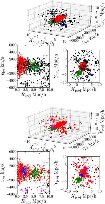
Figure 2. Same massive cluster shown in Figure 1, but now the galaxies are colored based on their membership to true 3D substructures (top) and 2D substructures identified by the  = 3 model (bottom). The true 3D substructures are identified as any ROCKSTAR halo gravitationally bound to the cluster that falls within the FOV of the cylindrical cut and has at least 10 galaxies.
Download figure:
Standard image High-resolution imageAs is obvious in Figure 2, each 2D substructure could include members from different 3D substructures or none, so we quantify the success rate of a 3D substructure identification. We also compare these results to a recent substructure identification method that utilizes the caustic technique (Yu et al. 2015, hereafter Y15). The method detailed in Y15 uses a preprocessing step of the caustic method to build a binary tree based on the projected binding energy between galaxies and groups of galaxies and then cuts the tree to identify substructures. They tested their methodology using the Coupled Dark Energy Cosmological Simulation (Baldi 2012), and they report that 49% of their identified 2D substructures contain at least one member of a 3D substructure and that 51% of the 2D substructures with at least one 3D member have 80% of their members belonging to the same 3D substructure. Here we will use the same metric they developed to compare our identification with theirs.
There are a few caveats we want to address before our discussion of the results. First, Y15 tested their substructure identification on dark matter particles in the simulation instead of galaxies painted onto subhalos as we do. Second, although our model is interested in identifying substructure, this is merely a secondary feature, not the main focus of our modeling framework. And finally, our model is restricted to a preset number of substructures, while the caustic method allows for any number of substructures; therefore, the substructures identified with our model are more likely to be larger and include galaxies from multiple 3D substructures. Despite these caveats, we will quantify the comparison between these two methods because the caustic technique substructure identifier is by far the most robust substructure identification model presented in the literature.
For each 2D substructure with at least one galaxy that is also a member of a 3D substructure, Y15 defines  as the largest fraction of its members that are also members of the same 3D substructure. Because our substructure model calculates the probability of membership posterior distributions for each galaxy for each 2D substructure, we identify the member galaxies of each 2D substructure with two methods. The first method (SUBMEM1) draws Nsamples = 10,000 samples from each galaxy's membership probability posterior distributions and assigns a membership to the 2D substructure with the highest probability of membership. Then, for each galaxy we take the mode of these samples to determine their final 2D substructure membership. This method will generate a 2D substructure membership for each galaxy. The second method (SUBMEM2) is more selective and only assigns a 2D substructure membership if the galaxy has a probability of membership
  (Equation (10)).
Using the SUBMEM1 method for substructure member identification, 59% of 2D substructures have at least one member of a 3D substructure. Compared to Y15's method (47%), the substructures identified with our modeling are more likely to have at least one member of a 3D substructure; however, this is a bit misleading. Because we fix the number of 2D substructures per model (and only allow upward of three substructures), the 2D substructures are more likely to be large and include many 3D substructures. This will inflate this percentage. This effect is best realized in the distribution of  , which is shown in Figure 3. Because each 2D substructure is large and could contain many 3D substructures, there are very few 2D substructures with large
  values when using the SUBMEM1 method for membership identification. The black curve in Figure 3 shows the cumulative distribution of
  , showing that our models have a median value of ∼0.40, whereas, compared to Y15 (shown in red), the caustic technique has a median value of 0.77. In other words, 50% of the 2D substructures identified using SUBMEM1 have only ∼40% of their member galaxies that are also members of the same bound 3D substructure. However, some of these galaxies included in each 2D substructure could have a low probability of memberships, which might be skewing this distribution. If this is the case, then SUBMEM2 (which only includes highly probable substructure members) should perform much better.
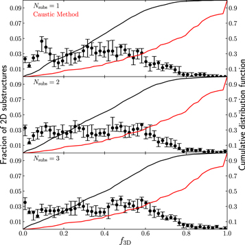
Figure 3. Distribution of  , the largest fraction of the total number of members of a 2D substructure that are also members of a single 3D substructure. Member galaxies of each 2D substructure were determined via the SUBMEM1 method. The panels are organized by the number of subpopulations allowed in each model. The error bars show the 10% and 90% limits derived from the 10 random samplings of each mock observation. The black line shows the cumulative distribution function of this distribution, while the red line shows the cumulative distribution function for
  using the caustic technique outlined in Y15.
Download figure:
Standard image High-resolution imageFor 2D substructure members identified by SUBMEM2, 53% of 2D substructures have at least one member of a 3D substructure. Furthermore, for these 2D substructures, 50% have  for the
  = 3 models, which is a slight improvement over Y15. The full distribution of
  for SUBMEM2 is shown in Figure 4. For
  our model is slightly outperformed by Y15, but the
  = 3 model has a small advantage over Y15. This clearly shows that, especially for the highly probable 2D substructure member galaxies, the 2D substructures identified in this model correlate with the true bound 3D substructures of the cluster.

Figure 4. Same as Figure 3, except we use the SUBMEM2 method to identify 2D substructure members.
Download figure:
Standard image High-resolution imageIdentifying substructure is merely an added bonus of the modeling framework; the main purpose is to measure more precise cluster masses while simultaneously accounting for substructure. In Section 4.4 we implement a dark matter halo model to fit real observations of A267 in order to fit the underlying dark matter mass profile of the cluster; however, this calculation is expensive and would be unfeasible to run over a large amount of mock observations. Therefore, here we will discuss the uniform velocity dispersion  as a proxy for cluster mass. Figure 5 shows the distribution
  as a function of true cluster mass M200c for all clusters. There is a well-established power-law scaling relationship between velocity dispersion and mass that dates back to Fritz Zwicky (Zwicky 1933) and is still commonly used today (e.g., Bocquet et al. 2015). This relationship is due to the virial theorem
  , but the power-law index is commonly a free parameter fit from data. The value of the power-law index is easy to fit; however, the scatter about the power-law relationship is of greater importance (Ntampaka et al. 2016).

Figure 5. Velocity dispersion of the main cluster halo  as a function of true cluster mass M200c from the MDPL2. Each column corresponds to the number of subpopulations
  allowed in each model. The top panels show the distribution of galaxies, clearly showing the high- and low-mass samples. Each point is colored depending on whether the cluster is relaxed (i.e., little to no significant substructure) or substructured. The error bars show the 10% and 90% ranges from the 10 random samplings of each cluster. Because there is a power-law relationship between velocity dispersion and mass, we fit a power law (blue dashed lines) with scatter (blue dotted lines). In the bottom panels we show the residuals and quantify the scatter of these residuals for the relaxed and substructured clusters, independently. As the number of subpopulations in the model increases, the fit scatter in the power law decreases, as does the residual scatter of substructured clusters.
Download figure:
Standard image High-resolution imageIn Figure 5 we fit a power law through the derived cluster velocity dispersion  as a function of true cluster mass M200c along with the scatter about this relationship. The power law is shown by the blue dashed lines, while the width of the fit scatter is shown by the blue dotted lines. Clearly, as we increase the number of subpopulations
  , the scatter decreases drastically. Furthermore, we separate the cluster sample into two groupings, relaxed and substructured, depending on the number of bound 3D substructures each cluster has. In the bottom panel, we show the residuals and the mean and standard deviation of the residual distributions for each grouping. This shows that the scatter in the residuals of the substructured cluster sample decreases by nearly 35% from the
  = 0 model to the
  = 3 model.
4. Application to A267
In this section we will apply the multipopulation model outlined in Section 2 above to spectroscopic observations of the galaxy cluster A267 (z ∼ 0.23). In Section 4.1, I will describe the data set. Section 4.2 will layout the contamination model used here. Section 4.3 will describe and present the results for the modeling assuming a uniform velocity dispersion for the main cluster halo. In Section 4.4 we apply a dark matter halo model in order to fit the mass profile of A267.
4.1. Observational Data Set
The A267 data are drawn from three separate catalogs. The spectroscopic observations are a combination of over 1000 measured redshifts by HectoSpec (HeCS; Rines et al. 2013) and 223 galaxies with the Michigan/Magellan Fiber System (M2FS). For galaxies that were observed in both data sets, we used a weighted (by inverse variance of redshift) mean of the measured redshifts. The combination of these included 1219 galaxy redshifts with a median error of 32 km s−1.
The observations, data reduction, and spectral fitting model for the M2FS spectroscopy are described in detail in Tucker et al. (2017). We fit these spectra using a population synthesis integrated light model, which estimates line-of-sight velocity,  , along with stellar population parameters mean age, metallicity
 ![$[\mathrm{Fe}/{\rm{H}}]$](https://content.cld.iop.org/journals/0004-637X/888/2/106/revision1/apjab609dieqn76.gif) , chemical abundance
, chemical abundance ![$[\alpha /\mathrm{Fe}]$](https://content.cld.iop.org/journals/0004-637X/888/2/106/revision1/apjab609dieqn77.gif) , and internal velocity dispersion
, and internal velocity dispersion  . A summary of these results can be found in Table 3 of Tucker et al. (2017), and the full data product, including sky-subtracted spectra with variances, best-fitting model, and samples from the posterior distribution, can be found online at doi:10.5281/zenodo.831784.
The HeCS catalog is described in detail by Rines et al. (2013) and contains redshifts for over 22,000 galaxies in over 50 different clusters. Compared to the M2FS sample, the HeCS sample for A267 is much larger and provides wider coverage. The M2FS sample, while smaller, provides extra dimensions of information, including mean ages and metallicities.
Both spectroscopic data sets were selected via the galaxy red sequence described in Section 2.1 of Tucker et al. (2017) and shown in Figure 1 of that paper. We applied this same selection criterion to obtain a photometric galaxy sample from the SDSS of 1849 galaxies. The galaxies contained in the spectroscopic sample are a subset of those in the photometric sample. Figure 9 shows the positions of all galaxies used in this analysis. The open markers are galaxies with only photometric observations, while the filled markers are galaxies with spectroscopically measured redshifts. Figure 10 shows the redshift distribution of galaxies used in this analysis.
Because we select galaxies via the red sequence, our inferences on cluster substructure and kinematics are biased to the quiescent galaxy population. We note that the velocity dispersion of quiescent galaxy members has been shown in the past to be smaller than the velocity dispersion of blue members (see, e.g., Zhang et al. 2012).
The spectroscopic completenesses as a function of radial distance and r-band magnitude are shown in Figure 6. The majority of the galaxies targeted via the red sequence lie between magnitudes 18 and 21.
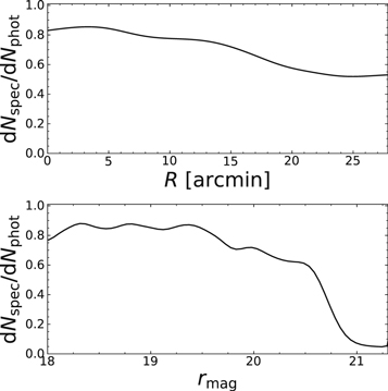
Figure 6. Spectroscopic completeness as a function of radial distance (top) and SDSS r-band magnitude (bottom).
Download figure:
Standard image High-resolution image4.2. Contamination Model
The gray histograms in Figure 10 show the velocity distribution of the A267 spectroscopic sample. The contamination population of galaxies (the numerous subpeaks throughout the distribution) is dominated by foreground and background groups and clusters of galaxies; therefore, extra care must be taken in determining the contamination model. To this end, we implement a modified version of the multipopulation model with the aim of fitting a fixed number of these contamination clusters and some uniform component on the sky. We fit the contamination model in advance using only galaxies without spectroscopic redshifts and galaxies with spectroscopic redshifts that are obvious contaminants (i.e., galaxies with line-of-sight velocities  km s−1).
The contamination model is of the same form as the multipopulation mixture model described in detail in Section 2, with a few minor changes. This model will be made up of Ncontam + 1 populations. The first population will be used to describe the field galaxies that will not be fit into a clustered population. Therefore, we assume that these galaxies will be uniformly distributed on the sky  , with a generalized gamma distribution used to describe the velocity distribution:
where p, a, and d are free parameters and Γ is the gamma function. This distribution was chosen for its flexibility to handle the redshift distribution of field galaxies in our sample; however, there is no physical motivation for the gamma distribution. We do not include observational errors in this velocity distribution because the distribution covers a large range in redshift space and so the relatively small velocity errors will have little effect on the underlying distribution. The remaining Ncontam populations are described by NFW light profiles with Gaussian velocity distributions. The free parameters used for this contamination model are listed and described in the top portion of Table 2.
Table 2. Free Parameters and Priors for Uniform Velocity Dispersion Model of A267
| Parameter | Prior | Description |
|---|---|---|
![${\mathrm{log}}_{10}\left[{{\rm{\Sigma }}}_{0}/{\mathrm{radians}}^{-2}\right]$](https://content.cld.iop.org/journals/0004-637X/888/2/106/revision1/apjab609dieqn81.gif)
|
Uniform between −2 and 15 | Light profile for uniform component of contamination model |

|
Uniform between −6 and 6 | Parameter of gamma distribution Equation (14) |

|
Uniform between −6 and 1 | Parameter of gamma distribution Equation (14) |

|
Uniform between −6 and 6 | Parameter of gamma distribution Equation (14) |
![${\mathrm{log}}_{10}\left[{r}_{s,\mathrm{contam},i}/{R}_{\max }\right]$](https://content.cld.iop.org/journals/0004-637X/888/2/106/revision1/apjab609dieqn85.gif)
|
Uniform between −3 and 0 | NFW scale radius of ith contamination population |
![${\mathrm{log}}_{10}\left[{r}_{c,\mathrm{contam},i}/{R}_{\max }\right]$](https://content.cld.iop.org/journals/0004-637X/888/2/106/revision1/apjab609dieqn86.gif)
|
Uniform between −3 and 0 | Radial offset of center of ith contamination population |

|
Uniform between 0 and 2π | Angular location of center of ith contamination population |

|
See Equation (15) | Redshift of ith contamination population |

|
Uniform between 0 and 3.5 | Velocity dispersion of ith contamination population |

|
Uniform between 0 and 1 | Number fraction hyperparameters for contamination model |
![${\mathrm{log}}_{10}\left[{{\rm{\Sigma }}}_{\mathrm{rs}}/{\mathrm{radians}}^{-2}\right]$](https://content.cld.iop.org/journals/0004-637X/888/2/106/revision1/apjab609dieqn91.gif)
|
Uniform between −1 and 1 | Rescale uniform component of contamination model |
| fcontam | Uniform between 0 and 1 | Number fraction of all contamination population |
![${\mathrm{log}}_{10}\left[{r}_{s,\mathrm{main}}/{R}_{\max }\right]$](https://content.cld.iop.org/journals/0004-637X/888/2/106/revision1/apjab609dieqn92.gif)
|
Uniform between −3 and 0 | NFW scale radius of main halo light profile |
![${\mathrm{log}}_{10}\left[{r}_{c,\mathrm{main}}/{R}_{\max }\right]$](https://content.cld.iop.org/journals/0004-637X/888/2/106/revision1/apjab609dieqn93.gif)
|
Uniform between −3 and 0 | Radial offset of center of main halo |

|
Uniform between 0 and 2π | Angular location of center of main halo |
| zmain | Uniform between 0.22 and 0.245 | Redshift of main halo 
|

|
Uniform between 0 and 3.5 | Velocity dispersion of main halo |
![${\mathrm{log}}_{10}\left[{r}_{s,\mathrm{sub},i}/{R}_{\max }\right]$](https://content.cld.iop.org/journals/0004-637X/888/2/106/revision1/apjab609dieqn97.gif)
|
Uniform between −3 and 0 | NFW scale radius of ith substructure light profile |
![${\mathrm{log}}_{10}\left[{r}_{c,\mathrm{sub},i}/{R}_{\max }\right]$](https://content.cld.iop.org/journals/0004-637X/888/2/106/revision1/apjab609dieqn98.gif)
|
Uniform between −3 and 0 | Radial offset of center of ith substructure |

|
Uniform between 0 and 2π | Angular location of center of ith substructure |

|
See Equation (12) | Velocity of ith substructure |

|
Uniform between 0 and 1 | Velocity dispersion of ith substructure |
| fi | Uniform between 0 and 1 | Number fraction hyperparameter |
Note. The first set of parameters (first 10 rows) are for the contamination model and are fit ahead of time using only obvious contamination galaxies. For the contamination model we use one uniform population and five NFW populations. The remaining free parameters are used to describe the kinematics of the cluster.
Download table as: ASCIITypeset image
For the same reasons discussed in Section 3.3, we use a nonuniform prior on the redshifts of the contamination populations:
where zmin and zmax are set by the full range of redshifts in our sample.
For this model we fit Ncontam = 5 contamination populations. These five populations are clearly visible in the velocity distribution of our sample (gray histograms), as well as the model fit in Figure 10. Although there are clearly more peaks in the velocity distribution that the model does not properly account for, it is unfeasible to fit those distributions because MultiNest becomes increasingly inefficient at sampling high-dimensional posteriors. In order to fit this model, we required ∼1.25 × 10⁹ likelihood evaluations with a sampling acceptance rate of 1.8 × 10⁻⁴, which took over 1.6 × 10⁴ CPU hours to fully sample the posterior distributions.
In order to cut down on the number of free parameters, we fit the contamination model beforehand and feed this fit model into the analysis described below. We originally sampled the posterior of the contamination model; however, this also drastically decreased the sampling efficiency, so instead we use the highest likelihood model from the fit instead. We have seen that there is no dependence on the resulting posterior distribution in spite of this choice.
4.3. Uniform Velocity Dispersion Profile
In this section we use a simple kinematic model in order to explore how inferences on the kinematics of A267 depend on the number of subpopulations allowed. We do this by running five separate model fits, each model allowing an additional subpopulation (from zero to four). The free parameters and their prior ranges used in these models are given in Table 2.
4.3.1. Model Setup
The model setup is similar to the setup described in Section 3.3, with a few minor differences mainly pertaining to the contamination model. We use the pre-fit contamination model described in Section 4.2, which drastically reduces computation time and increases computation efficiency. Although the contamination model is already fit, we do allow there to be a rescaling of the uniform contamination component Σrs. The remaining free parameters are discussed in detail in Section 3.3. We again use the same prior on the line-of-sight velocities of the subpopulations in order to preserve prior probability mass and solve the identifiability issue (Equation (12)). The transformations from the number fraction hyperparameters to the true number fractions are given by
In total these models are described by  free parameters. For the A267 sample we include Ngal = 1675 galaxies in the photometric sample, with Nspec = 1121 of these galaxies with spectroscopically measured line-of-sight velocities.
4.3.2. Substructures in A267
As discussed in Old et al. (2018), the presence of substructure can have a significant effect on dynamical mass measurements of galaxy clusters. In order to understand this effect on mass estimates, we first assume a simple uniform velocity dispersion profile to explore how substructure influences these measurements. We fit a set of five models, with each model allowing an additional subpopulation within the cluster environment (the largest number of subpopulations we fit is  = 4).
= 4).
Figure 7 shows a summary of the main results from this analysis in black. In the top panel we show the evolution of the change in the log evidence for each model relative to a model with one fewer subpopulation. This value is frequently referred to as the Bayes factor, and it is commonly used for model selection. The larger the Bayes factor, the more significant the evidence is that the new model is "better" than the previous model, accounting for differences in model complexity. According to Kass & Raftery (1995), a Bayes factor ( ) between 3 and 5 indicates "strong" evidence, and if this factor exceeds 5, then the new model is very strongly favored. The Bayes factor is consistently >5 for the
  = 1, 2, and 3 models, which indicates that each of these models is strongly favored over the model with one less subpopulation (
 = 0, 1, and 2, respectively). However, the
  = 4 model (with Bayes factors <3) is only "slightly positive" or "not worth more than a bare mention" compared to the
  = 3 model.

Figure 7. Summary plot of the subpopulation analysis, with the black curves showing the progression for the uniform velocity dispersion models, while red is for the dark matter halo models. The top panel shows the evolution of the change in Bayesian evidence relative to a model with one fewer subpopulation, which is commonly known as the Bayes factor. The second panel shows the number of likelihood evaluations required to adequately sample the posterior pdf of each model. Next is the number fraction of galaxies within all subpopulations. The bottom four panels are the model parameters used to describe the main cluster populations: NFW scale radius  , mean cluster redshift
  , velocity dispersion
  , and mass M200 and concatenation c200 for the dark matter model. The dashed line in the fifth panel shows the measured redshift of the BCG for A267. In the sixth panel, the green star shows the velocity dispersion of A267 as measured by Rines et al. (2013).
Download figure:
Standard image High-resolution imageThe second panel in Figure 7 shows the number of likelihood evaluations needed to adequately sample the posterior probability density function (pdf) of each model. As expected for models with an increasing number of free parameters, the required number of likelihood evaluations increases exponentially, rendering the computation of increasing numbers of subpopulations  expensive.
The third panel in Figure 7 shows the number fraction of galaxies in all subpopulations. This panel gives an idea of how many galaxies are added to the subpopulations with an increasing number of subpopulations.
In the next three panels of Figure 7 we show the evolution of free parameters describing the main cluster: NFW scale radius  , mean cluster redshift zmain, and uniform velocity dispersion
  . The sixth panel (
 ) shows the evolution of velocity dispersion, a proxy for cluster mass. For comparison, we include the velocity dispersion for A267 measured by Rines et al. (2013), which is calculated by first identifying cluster members via the Caustic technique (Diaferio & Geller 1997) and calculating the dispersion of the members about the mean cluster redshift (also determined via the Caustic method). The Caustic method does not explicitly consider the effects of substructure (unless it is evident in the plane of
  ), so we compare it to our measurement assuming
  = 0, finding good agreement. As the number of subpopulations increases, the velocity dispersion trends downward; furthermore, the velocity dispersion decreases by ∼400 km s−1 from
  = 3 to
  = 4 (see below for more details on this drop-off).
The inflation of velocity dispersion due to the presence of substructure is not a new result. Beers et al. (1982) studied the dynamics of A98 and showed that the cluster was substructured with two distinct components. Furthermore, by using a two-component model to fit the cluster dynamics, they showed that failure to recognize this substructure inflates the velocity dispersion and hence the mass-to-light ratio of the cluster. Geller (1984) obtains a similar result for the Cancer Cluster. What is new here is the ability to evaluate the number of substructures and estimate cluster mass while marginalizing over uncertainty in the substructure parameters.
As the number of subpopulations increases, the scale radius  decreases for the most part. This trend is consistent with the mass of the main cluster also decreasing. While the redshift of the cluster stays roughly constant throughout most of the models, it is significantly lower than the redshift of the BCG of A267, which is shown as the black dashed line in Figure 7. This offset is on the order of ∼100 km s−1 and could be interesting with regard to tests of a "wobbling" BCG as predicted by SIDM (Harvey et al. 2017; Kim et al. 2017).
There is clearly something different happening from  = 3 to
  = 4, so let us look more into that now. Figure 8 shows the distributions of galaxies on the sky and in phase space. Each galaxy is colored by their memberships to a given population. The galaxy members were determined via the SUBMEM2 method discussed above, which assigns membership to a population if a galaxy has a probability of membership that exceeds 0.9. If a galaxy's probability of membership is below this threshold for all populations, then it is labeled as a contamination galaxy. We showed in Section 3.4 that this prescription for identifying substructure members yields a strong correlation to the true 3D substructures for mock observations from simulations.
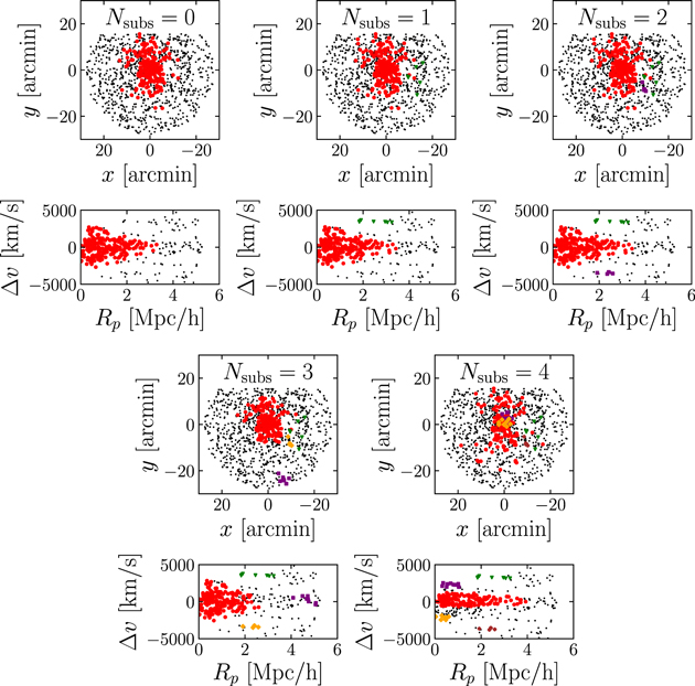
Figure 8. Sky position and phase-space diagrams for the A267 sample from the uniform velocity dispersion models. Each galaxy is colored based off of their membership to each substructure. Black galaxies are contamination galaxies, red are main cluster halo galaxies, and green, purple, orange, and brown are the four substructures fit in the models. The panels are organized by increasing number of substructures accounted for in the model.
Download figure:
Standard image High-resolution imageIn the  = 0 panels, the cluster and its trumpet-shaped caustic are clearly visible. The first substructure the model fits is an elongated grouping of galaxies with a center x ∼ −15' and velocity offset ∼+4000 km s−1 relative to the cluster. The second substructure found is a small localized group of galaxies that also has a large velocity offset relative to the cluster (∼−4000 km s−1). An important feature to note is that the subpopulation identified in the
  = 1 model is still identified as a distinct substructure in the
  = 2 model. This is important because each model is independent of the previous one; there is no guarantee that the identification of the substructure will be consistent. The third subpopulation identified a localized group of galaxies at a large projected radius of ∼5 Mpc h−1 but at a similar redshift to the cluster. These galaxies are likely an infalling group of galaxies to A267. Once this substructure is modeled accordingly, the cluster light profile is more compact, yet the velocity dispersion increases slightly.
The  = 4 model yields an odd result that is actually expected once the assumptions of the model are considered. With the added complexity of the fourth substructure and the requirement that the velocity dispersion of the cluster is constant, the model essentially overfits the distributions. This can easily be seen in the striped pattern in the
  = 4 phase-space panel of Figure 8. The cluster's light profile is much larger now and the velocity dispersion is much smaller because the model can easily fit a small uniform dispersion profile while accepting the tails as independent substructures. There are sets of galaxies that were once highly probable members of the main cluster that are now no longer highly probable members of any population. The Bayesian evidence (top panel of Figure 7) does not favor this model over the
  = 3 model; however, this could change once we incorporate a more realistic velocity dispersion profile, as will be discussed in Section 4.4 below.
Table 3 gives a summary of the results for the  = 3 model. The parameters describing the main cluster halo all have strong constraints; furthermore, the center of the main halo's light profile is offset from the BCG of A267 by 89.9 ± 14.2 kpc h−1. The scale radii of the substructures are relatively unconstrained mainly because of the low number of galaxies in each population. The scale radius of the first subpopulation is completely unconstrained. This is likely due to the fact that the galaxies in this population (see Figure 9) are elongated on the sky and therefore are not fit well by the radially symmetric NFW profile. Despite the poor fits to the light profile, the central locations, redshifts, and velocity dispersions of the substructures are relatively well constrained.

Figure 9. Top left: positions of galaxies on the sky. Each galaxy is colored and shaped based on which population in which the galaxy has the highest probability of membership: red circles are the main cluster population; green triangles, purple squares, and orange diamonds are for the three subpopulations; and blue stars are either foreground or background contamination galaxies. The solid red circle shows the scale radius of the main cluster population  centered on A267. The other colored circles show the scale radius
  of their respective subpopulations centered on the measured center of the population. The dashed black curves show contours of equal density from the highest likelihood number density profile to the data (
 ). In the other two panels, we overplot these contours, as well as the scale radii of the populations on top of the SDSS image center on A267, the X-ray luminosity (shown as a pink hue), and the weak-lensing signal (Okabe et al. 2010; shown in light blue). The bottom panel is a zoom-in on the center of A267.
Download figure:
Standard image High-resolution imageTable 3.
Mean Values and Standard Deviations of 1D Posterior pdf's for A267 Free Parameters in the Uniform Velocity Dispersion  Model
Model

|

|

|
z |

|
fmem | Nmem | |
|---|---|---|---|---|---|---|---|
| Main | 357 ± 68 | 28.174 ± 0.001 | 0.999 ± 0.001 | 0.2288 ± 0.0003 | 951 ± 56 | 0.199 ± 0.012 | 183 ± 22 |
| Sub1 | 930 ± 692 | 27.964 ± 0.048 | 0.944 ± 0.075 | 0.2403 ± 0.0004 | 229 ± 96 | 0.014 ± 0.005 | 8 ± 3 |
| Sub2 | 247 ± 269 | 28.070 ± 0.032 | 0.625 ± 0.105 | 0.2297 ± 0.0016 | 429 ± 124 | 0.015 ± 0.006 | 7 ± 3 |
| Sub3 | 54 ± 189 | 28.022 ± 0.057 | 0.864 ± 0.042 | 0.2173 ± 0.0003 | 131 ± 74 | 0.006 ± 0.002 | 5 ± 1 |
Download table as: ASCIITypeset image
Figure 9 shows a more in-depth look at the sky positions of the galaxies labeled by their most likely substructure membership for the  = 3 model. In the top left panel, we show just the sky position of our sample. Galaxies with colors and various shapes are ones with spectroscopic redshifts and colored based off of their membership. The black points are galaxies without spectra that were used to constrain the light profiles in the model. The contours show the light profile fit from the model of all populations (contamination + main cluster + substructures). The other two panels show an overlay image of our analysis (the colored circles and white contours) with the SDSS mosaic (Blanton et al. 2017), the weak-lensing signal in blue (Okabe et al. 2010), and X-ray luminosity in pink (XMM-Newton ObjID 0084230401). The bottom panel is a zoom-in on the central core of A267.
In Figure 10 we show the velocity distribution of our sample. We overplot the velocity distributions fit to the data for the  = 3 model. The darker and lighter regions of these distributions show the inner 68% and 95% limits of the posterior distributions, respectively. The contamination model (blue) fits the five strongest subpeaks in this distribution, with the gamma distribution doing a good job fitting the broad distribution of field galaxies. The inset in the upper left corner shows a zoom-in of the distribution around the mean redshift of A267, which shows in greater detail the velocity distributions of the main halo and substructures.
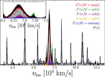
Figure 10. Velocity distribution profile. The gray histograms show the profile of the galaxy redshift sample (HeCS plus M2FS). The red curve is the profile for the main cluster population; the green, purple, orange, brown, and cyan curves are for the five subpopulations; and the blue curve is for the contamination population. The black curve is the sum of all of these profiles. The inset in the upper left corner shows the distribution zoomed in on the region of redshift space around A267.
Download figure:
Standard image High-resolution image4.3.3. Comparison to Other Test for Substructures
A commonly used statistical test for substructure is known as the Δ-statistic and was developed by Dressler & Shectman (1988). The Δ-statistic looks for deviations in the local velocity from the global velocity of the cluster. First, for each galaxy one calculates the mean local velocity vlocal and local dispersion σlocal of the n nearest neighbors to the galaxy, where typically  . This local velocity and dispersion are compared to the global velocity
  and dispersion
  of the cluster quantified by
The full Δ-statistic is the sum of  over all galaxies Ntot.
The Δ-statistic is used to test whether or not there is considerable substructure within the cluster's environment. According to Dressler & Shectman (1988), for a relaxed cluster without significant substructure Δ ∼ Ntot. Figure 11 shows a "bubble plot," a commonly used representation of the Δ-statistic. Each galaxy's "bubble" is sized by that galaxy's δi value given by Equation (17). In each panel we show the progression of this plot for an increasing number of subpopulations. We use the SUBMEM2 method of cluster member identification by applying a hard cut on the probability of membership in the main cluster  and only show galaxies with
  . In the upper left corner we also show the ratio Δ/Ntot in order to show a quantitative comparison between the two methods. As the number of substructures increases to
  = 3, the ratio of
  is slightly closer to 1, yet it is still larger, suggesting that there may be additional substructures. This is also noticeable qualitatively by the overall decrease in size of the δ-bubbles. However, this ratio increases to its largest value for the
  = 4 model, suggesting that the substructures identified by this model are likely not real, as already discussed above. The main takeaway from this comparison is that our model is improving the Δ-statistic; however, it is limited by the uniform velocity dispersion profile, which affects the identification of additional substructures for the
  = 4 model.
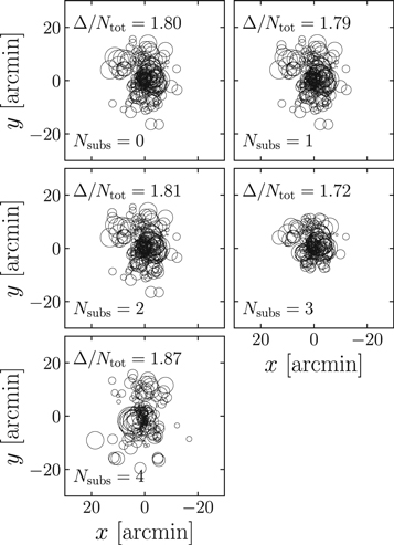
Figure 11. "Bubble plot" for the Δ-statistic. Each member galaxy is plotted with a circle whose size is proportional to  (Equation (17)). Regions of large circles show areas with high probability of substructure. From left to right and top to bottom we increase the number of subpopulations, which is given in the lower left corner of each panel.
Download figure:
Standard image High-resolution imageWe also make a qualitative comparison of the substructures identified with the  = 3 model to the binary tree algorithm of Yu et al. (2015). The sky positions and phase-space diagrams for both sets of substructures are shown in Figure 12. There is some agreement between the main cluster halos (red circles) and the purple substructure. The main cluster identified with the
  = 3 model has a more concentrated distribution albeit with a broader velocity dispersion. The purple substructure identified by the binary tree method is more extended on the sky compared to a similar substructure identified by the
  = 3 model. Interestingly, the cyan and orange substructures from the binary tree method do have some overlap with two of the substructures from the
  = 4 model (see Figure 8). We will revisit this comparison below while discussing the results of the model using a radial velocity dispersion profile as opposed to a uniform profile used here.
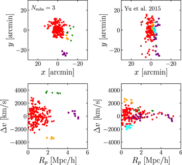
Figure 12. Comparison of the  = 3 model's substructures (left) with those identified by the binary tree method (Yu et al. 2015; right). The top panels show the sky positions of the galaxies, while the bottom panels show the phase-space diagrams.
Download figure:
Standard image High-resolution image4.4. Dark Matter Halo Model
Thus far we have assumed that A267's velocity distribution is independent of radius. In the following subsections, we describe our procedure and results for fitting a dark matter halo model and corresponding velocity dispersion profile to the main cluster population of A267 ( ). We will first describe the theoretical framework for calculating the velocity dispersion profile as a proxy for cluster mass using the spherical Jeans equation, and then we will describe how we implement this technique for A267.
4.4.1. Jeans Analysis
In order to measure cluster mass, we assume that the galaxies within the main cluster population sample a single, pressure-supported halo that is dynamically relaxed and traces an underlying dark-matter-dominated gravitational potential. With the additional assumption of spherical symmetry, the mass profile, M(r), of the dark matter halo relates to the galaxy distribution function via the Jeans equation:
where  is the 3D galaxy number density,
  is the radial velocity dispersion, and
  is the orbital anisotropy. Using cosmological dark-matter-only simulations, Wojtak et al. (2013) showed that the velocity anisotropy for cluster-sized halos (1014–1015 h−1 M⊙) is roughly constant with radius at a value β ∼ 0.4. According to Binney & Tremaine (2008), for the special case of constant, nonzero anisotropy, the Jeans equation has the simple solution

And by projecting along the line of sight, we can relate the mass profile to the observable profiles of the projected galaxy number density I(R) and velocity dispersion profile σp(R) by
And so, by plugging Equation (19) into Equation (20), specifying an underlying dark matter halo model M(R), and adopting a profile for I(R), we can determine the velocity dispersion and mass profiles of the cluster.
For simple anisotropy profiles, we can rewrite the combination of Equations (19) and (20) as
where the kernel K depends on the choice of anisotropy and is given for five anisotropy models in Appendix 2 of Mamon & Łokas (2005). For A267, we used a constant anisotropy model. Although it is not the most physically motivated model, we use a Gaussian velocity distribution similar to Mamon et al. (2013) because it is easy to implement numerically and is a fairly good approximation for the observed profile of galaxy clusters.
4.4.2. Model Setup
The modeling setup for the radial velocity dispersion profile is similar to the uniform dispersion setup especially in terms of the contamination model and substructures. Similar to before, we still assume that the number density profile of the main cluster halo follows an NFW profile, but now there is an underlying dark matter halo that we also assume is NFW in shape. These profiles will have the same centers but could have different scale radii. For the dark matter halo, the dark matter NFW profile ρ(r) is related to the mass profile by  .
.
The dark matter halo is parameterized by two free parameters: M200 = M(r200) and c200 = r200/rs, where r200 is the radius at which the mean density falls to 200 times the critical density of the universe. For the Jeans analysis, we parameterize the model by the velocity anisotropy index β, which we assume to be uniform. The anisotropy index varies from  for completely tangential orbits to +1 for purely radial orbits. Because of this large parameter space, we reparameterize the anisotropy index so that
  , which we constrain to vary between −1 < β' < +1.
Altogether this model will include two free parameters for the contamination model (in addition to the pre-fit contamination model described in Section 4.2), seven free parameters for the main cluster halo, and six free parameters for each substructure. All free parameters and the adopted priors are listed in Table 4. Similar to before, the transformation from the number fraction hyperparameters to the number fractions of each population is given by Equation (16).
Table 4. Free Parameters and Priors for Dark Matter Halo Model of A267
| Parameter | Prior | Description |
|---|---|---|
![${\mathrm{log}}_{10}\left[{{\rm{\Sigma }}}_{0}/{\mathrm{radians}}^{-2}\right]$](https://content.cld.iop.org/journals/0004-637X/888/2/106/revision1/apjab609dieqn163.gif)
|
Uniform between −2 and 15 | Light profile for uniform component of contamination model |

|
Uniform between −6 and 6 | Parameter of gamma distribution Equation (14) |

|
Uniform between −6 and 1 | Parameter of gamma distribution Equation (14) |

|
Uniform between −6 and 6 | Parameter of gamma distribution Equation (14) |
![${\mathrm{log}}_{10}\left[{r}_{s,\mathrm{contam},i}/{R}_{\max }\right]$](https://content.cld.iop.org/journals/0004-637X/888/2/106/revision1/apjab609dieqn167.gif)
|
Uniform between −3 and 0 | NFW scale radius of ith contamination population |
![${\mathrm{log}}_{10}\left[{r}_{c,\mathrm{contam},i}/{R}_{\max }\right]$](https://content.cld.iop.org/journals/0004-637X/888/2/106/revision1/apjab609dieqn168.gif)
|
Uniform between −3 and 0 | Radial offset of center of ith contamination population |

|
Uniform between 0 and 2π | Angular location of center of ith contamination population |

|
See Equation (15) | Redshift of ith contamination population |

|
Uniform between 0 and 3.5 | Velocity dispersion of ith contamination population |

|
Uniform between 0 and 1 | Number fraction hyperparameters for contamination model |
![${\mathrm{log}}_{10}\left[{{\rm{\Sigma }}}_{\mathrm{rs}}/{\mathrm{radians}}^{-2}\right]$](https://content.cld.iop.org/journals/0004-637X/888/2/106/revision1/apjab609dieqn173.gif)
|
Uniform between −1 and 1 | Rescale uniform component of contamination model |
| fcontam | Uniform between 0 and 1 | Number fraction of all contamination population |
![${\mathrm{log}}_{10}\left[{r}_{s,\mathrm{main}}/{R}_{\max }\right]$](https://content.cld.iop.org/journals/0004-637X/888/2/106/revision1/apjab609dieqn174.gif)
|
Uniform between −3 and 0 | NFW scale radius of main halo light profile |
![${\mathrm{log}}_{10}\left[{r}_{c,\mathrm{main}}/{R}_{\max }\right]$](https://content.cld.iop.org/journals/0004-637X/888/2/106/revision1/apjab609dieqn175.gif)
|
Uniform between −3 and 0 | Radial offset of center of main halo |

|
Uniform between 0 and 2π | Angular location of center of main halo |
| zmain | Uniform between 0.22 and 0.245 | Redshift of main halo 
|
![${\mathrm{log}}_{10}[{M}_{200}/{M}_{\odot }\,{h}^{-1}]$](https://content.cld.iop.org/journals/0004-637X/888/2/106/revision1/apjab609dieqn178.gif)
|
Uniform between 13 and 16 | Mass of cluster interior to r200 |
![${\mathrm{log}}_{10}[{c}_{200}]$](https://content.cld.iop.org/journals/0004-637X/888/2/106/revision1/apjab609dieqn179.gif)
|
Uniform between 0 and 2 | Concentration of dark matter halo: 
|
![$-{\mathrm{log}}_{10}[1-\beta ]$](https://content.cld.iop.org/journals/0004-637X/888/2/106/revision1/apjab609dieqn181.gif)
|
Uniform between −1 and +1 | Anisotropy index β of velocity dispersion profile |
![${\mathrm{log}}_{10}\left[{r}_{s,\mathrm{sub},i}/{R}_{\max }\right]$](https://content.cld.iop.org/journals/0004-637X/888/2/106/revision1/apjab609dieqn182.gif)
|
Uniform between −3 and 0 | NFW scale radius of ith substructure light profile |
![${\mathrm{log}}_{10}\left[{r}_{c,\mathrm{sub},i}/{R}_{\max }\right]$](https://content.cld.iop.org/journals/0004-637X/888/2/106/revision1/apjab609dieqn183.gif)
|
Uniform between −3 and 0 | Radial offset of center of ith substructure |

|
Uniform between 0 and 2π | Angular location of center of ith substructure |

|
See Equation (12) | Velocity of ith substructure |
![${\mathrm{log}}_{10}[{\sigma }_{\mathrm{sub},i}/\mathrm{km}\,{{\rm{s}}}^{-1}]$](https://content.cld.iop.org/journals/0004-637X/888/2/106/revision1/apjab609dieqn186.gif)
|
Uniform between 0 and 3 | Velocity dispersion of ith substructure |
| fi | Uniform between 0 and 1 | Number fraction hyperparameter |
Note. The first set of parameters (first 10 rows) are for the contamination model and are fit ahead of time using only obvious contamination galaxies. For the contamination model we use one uniform population and five NFW populations. The remaining free parameters are used to describe the kinematics of the cluster.
Download table as: ASCIITypeset image
4.4.3. Results for A267
The red curves in Figure 7 show the progression of model parameters as the number of substructures is increased from  = 0 to
  = 4. There is a similar behavior for this set of modeling compared to the uniform velocity dispersion models. From
  = 0 to
  = 1 the Bayes factor (top panel) increases considerably, which indicates that the
  = 1 model is favored between the two. This trend continues with the
  = 2 model, and although the Bayes factor is not quite as large for the
  = 3 model, it still exceeds 5, providing strong evidence in favor of this model over models with fewer substructures. Unlike the uniform velocity dispersion models, which do not favor the
  = 4 model, there is strong evidence in support of the
  = 4 model with a dark matter halo.
The remainder of the parameters follow a similar trend to the uniform dispersion analysis except for the  = 4 models. In the dark matter halo model when
  = 4, the results are more consistent with the results from the models with fewer substructures. Furthermore, the mass of the cluster (sixth panel) decreases continuously and at a relatively steady rate as the number of substructures increase. The velocity offset from the BCG of A267 to mean redshift of the cluster remains roughly constant at ∼150 km s−1; however, the mean velocity of the cluster decreases slightly for the
  = 4 model, mainly due to the fact that the mean velocity of the additional substructure identified populates the high-velocity tail of the cluster's distribution.
Figure 13 shows the progression of substructure membership for an increasing number of substructures. This figure is similar to Figure 8, except for the choice of velocity dispersion profile. Both dispersion profiles yield two similar substructures, the green and purple populations seen in the  = 2 panels of both figures. One significant difference is that, with the radial dispersion profile used here, there are now main halo members beyond 4 Mpc h−1, unlike in the uniform dispersion models. In the
  = 3 and 4 panels, there is one fewer substructure identified than the model allows. This is due to the fact that posterior distribution for the additional substructure is highly multimodal, and so the procedure we use to identify cluster members essential finds no members of these populations. If, instead of sampling the posterior, we used just one sample, then there would be the proper number of substructures in all panels of Figure 13.
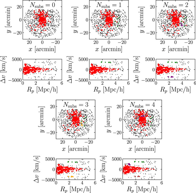
Figure 13. Same as Figure 8, except now for the dark matter halo models.
Download figure:
Standard image High-resolution imageFigure 14 shows the 1D and 2D posterior distributions for three parameters describing the subpopulations in the  = 3 (top) and
  = 4 models (bottom). The colors of each posterior correspond to the colors of the substructures shown in Figure 13. The purple and yellow posteriors in the
  = 3 and 4 panels, respectively, are unconstrained, which is why there are no member galaxies identified for these substructures in Figure 13. This multimodal behavior is typically indicative of at least one additional substructure that the model does not have the flexibility to fit because the number of substructures is fixed for each model. Nevertheless, the main goal of this modeling framework is to measure cluster masses while marginalizing over potential substructure, which is still achieved even though these parameters are unconstrained.
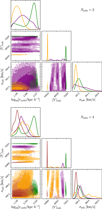
Figure 14. 2D and 1D posterior distributions for subpopulations inferred from the  = 3 (top) and
  = 4 (bottom) models. The colors of each distribution correlate to the colors of the substructures shown in Figure 13.
Download figure:
Standard image High-resolution imageFigure 15 shows the 1D and 2D posterior distributions for the parameters that define the main cluster population in the  = 4 model. The main cluster halo parameters are all reasonably well constrained. Table 5 lists a summary of the results for these parameters, as well as the parameters describing the substructures. It is clear from this table that Sub3 (the yellow distributions in Figure 14) is largely unconstrained. Furthermore, as is the case for the uniform dispersion models, the estimates on the NFW scale radii of the substructures' light profiles are largely uncertain owing to the low number of highly probable members in these populations.
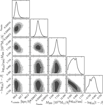
Figure 15. Posterior pdf's of parameters specifying the dark matter halo of A267, using the Jeans equation analysis described in Section 4.4. We show the scale radius of the NFW light profile  , mean cluster redshift zmain, virial mass and concentration of the dark matter halo M200 and c200, and velocity anisotropy β. We also show the 1σ, 2σ, and 3σ contours for the 2D posteriors.
Download figure:
Standard image High-resolution imageTable 5.
Mean Values and Standard Deviations of 1D Posterior pdf's for A267 Free Parameters in the Dark Matter Halo  Model
Model

|

|

|
z |

|
|

|
β | fmem | Nmem | |
|---|---|---|---|---|---|---|---|---|---|---|
| Main | 388 ± 87 | 28.174 ± 0.001 | 0.999 ± 0.001 | 0.2288 ± 0.0003 | 7.0 ± 1.3 | 0.71 ± 0.38 | −1.3 ± 2.1 | 0.192 ± 0.013 | 194 ± 24 | |
| Sub1 | 790 ± 703 | 27.974 ± 0.047 | 0.949 ± 0.061 | 0.2404 ± 0.0003 | 188 ± 72 | 0.013 ± 0.004 | 8 ± 3 | |||
| Sub2 | 110 ± 202 | 28.150 ± 0.016 | 1.066 ± 0.028 | 0.2363 ± 0.0020 | 235 ± 97 | 0.009 ± 0.004 | 5 ± 2 | |||
| Sub3 | 198 ± 404 | 28.115 ± 0.204 | 0.865 ± 0.204 | 0.2241 ± 0.0045 | 339 ± 224 | 0.011 ± 0.007 | 4 ± 3 | |||
| Sub4 | 34 ± 43 | 28.016 ± 0.003 | 0.859 ± 0.003 | 0.2173 ± 0.0002 | 100 ± 36 | 0.006 ± 0.002 | 5 ± 0 |
Download table as: ASCIITypeset image
In Figure 15, there is a strong c200–β degeneracy and a weaker  degeneracy. The
  relation is a usefully cosmological scaling relation that exhibits relatively low scatter. In Figure 16 we zoom in on the
  panel and compare the results from the dark matter halo models with predictions of the
  relation derived from N-body simulations (Dutton & Macciò 2014; Diemer & Kravtsov 2015). Even though the mass of the dark matter halo decreases with increasing number of subpopulations and the posterior for c200 is relatively less constrained, we still recover a mean concentration in accordance with Dutton & Macciò (2014).
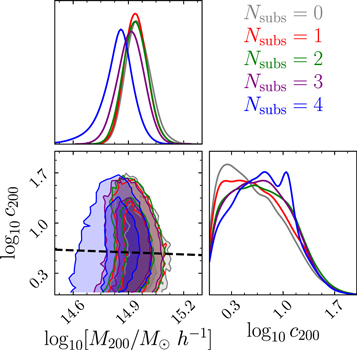
Figure 16. Mass–concentration posteriors from the dark matter halo models. Each color represents a model that allows for a different number of subpopulations. The dashed black curve shows the  relation from Dutton & Macciò (2014) and Diemer & Kravtsov (2015).
Download figure:
Standard image High-resolution imageFigure 17 shows the velocity dispersion profile  inferred from the Jeans analysis of A267. The dark and light shaded regions show the 68% and 95% confidence intervals of the posterior pdf's, respectively, while the black curve show the median posterior velocity dispersion profile. In red we compare the fit velocity dispersion profile to the binned velocity dispersion calculated with highly probable member galaxies (
 ). In the infall region of A267 (Rp ≳ 2 Mpc h−1), the fit dispersion profile exceeds the binned data. This is likely due to an inhomogeneity of the galaxy distribution in the cluster outskirts (Yu et al. 2016; Liu et al. 2018). The assumptions made when conducting a Jeans analysis break down at these radii, thus yielding a poor fit.
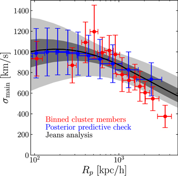
Figure 17. Line-of-sight velocity dispersion profile for A267 with the  = 4 model. The dark and lighter regions correspond to 1σ and 2σ of the posterior, respectively. The solid black line is the median posterior curve. The red points show the velocity dispersion of binned member galaxies. The blue points show the binned velocity dispersion calculated with simulated data generated from sampling the posterior distribution.
Download figure:
Standard image High-resolution imageIn order to qualitatively show any potential bias in calculating a binned velocity dispersion, we check the binning procedure using mock data generated from halo models sampled from the posterior. At each sample of the posterior, a catalog of galaxies is generated. These galaxies are then binned, and a velocity dispersion is calculated in the same way as the real data. The blue points show the results of this posterior predictive check. The error bars are calculated from the scatter of the velocity dispersion within each bin across the sampled posterior. The posterior predictive check shows almost no bias in the binned dispersion; however, there is considerably larger scatter within each bin than would be expected from the 1σ and 2σ widths of the posterior.
Figure 18 shows the mass profile of the dark matter halo for A267. Like previous plots, the dark and light regions show the 68% and 95% confidence intervals of the pdf's, respectively, and the solid black curve shows the median posterior. For comparison we include previous mass measurements of A267 from a variety of different techniques: in green the weak-lensing mass  (Okabe & Smith 2016), in red and purple the caustic mass
  and viral mass calculated with velocity dispersion of cluster members
  , respectively (Rines et al. 2013), and in blue the X-ray-derived mass MX500 (Jiménez-Bailón et al. 2013). Our results are consistent with MX500,
  , and
, and  , but we measure a significantly smaller mass than
  because the mass estimate derived from the velocity dispersion is more susceptible to substructure. Also shown in Figure 18 are the median posterior curves of the mass profile from the models with fewer substructures. For A267, as the number of substructures increases, the mass of the cluster decreases.

Figure 18. Projected radial mass profile for A267 with the  = 4 model. The darker and lighter regions correspond to 1σ and 2σ of the posteriors, respectively. The solid black line is the median posterior curve. The colored points show four different mass estimates of A267 from weak lensing (Okabe & Smith 2016; green), caustic (Rines et al. 2013; red), velocity dispersion (Rines et al. 2013; purple), and X-ray (Jiménez-Bailón et al. 2013; blue). Also shown, as the black curves, are the mass profiles for the models with fewer substructures.
Download figure:
Standard image High-resolution image
5. Conclusions
We have developed a multipopulation mixture model in order to simultaneously model the internal kinematics and substructure of A267. We included in this model the ability to fit Nsubs subpopulations, as well as cluster parameters such as NFW scale radius, mean cluster redshift, and velocity dispersion. We embedded this model in a full Bayesian framework, such that we quantify posteriors of all free parameters, as well as parameter covariances. In the application of this model to A267, we considered two alternative models that differ in how the cluster velocity dispersion is treated. We first assumed a simple uniform velocity dispersion profile to analyze the dependence of the internal kinematics on the arbitrary choice of the number of subpopulations. We then solved the spherical Jeans equation in order to fit a dark matter halo to A267, thus inferring the enclosed mass profile while allowing the velocity dispersion to vary with radius.
Prior to the work with A267, we tested the uniform velocity dispersion model with mock redshift observations from the dark-matter-only simulation MultiDark (MDPL2; Klypin et al. 2016). This allowed a comparison of the identified 2D substructures from this model with the true 3D substructures within the cluster environment known from the simulation. By comparing galaxies identified by the models as highly probable members to the 2D substructures, we report that 53% of the 2D substructures have at least one member galaxy that is also a member of a true 3D substructure. Furthermore, 51% of these 2D substructures have  (the largest fraction of the total number of members of a 2D substructure that are also members of a single 3D substructure). Both these values are on par with the current most robust cluster substructure identification algorithm (Yu et al. 2015, 2018); furthermore, our modeling framework simultaneously fits light and mass profiles of the cluster, which is lacking in the caustic methods.
The main focus of this modeling framework is to estimate more accurate cluster masses while accounting for the potential of substructure. To this end we showed with the mock observations from MDPL2 that there is significantly less scatter in the M200c–σ power-law relation when accounting for three additional substructures compared to a similar model that does not account for substructure (Figure 5). Furthermore, the majority of the decrease in scatter can be attributed to the clusters that exhibit significant amounts of true 3D substructures.
For A267, we investigated the dependence of the internal kinematics on the number of subpopulations. We showed that as the number of subpopulations increases, the inferred scale radius and velocity dispersion of the cluster both decrease, with significant consequences for cluster mass estimates (Figure 7). For the uniform velocity dispersion model the Bayes factor shows the largest evidence in favor of the  = 3 model; however, for the dark matter set of models
  = 4 is most favored. Comparing the preferred dark matter model
  = 4 to a dark matter model without substructure, we infer a dynamical mass that is ∼22% smaller than the model that neglects substructures. Furthermore, we found that the mean redshift of the cluster is also sensitive to the presence and treatment of subpopulations. This demonstrates how accounting for substructure can have significant implications for detecting "wobble" of the BCG around the cluster core, as predicted by self-interacting dark matter models (Harvey et al. 2017; Kim et al. 2017).
We compared the substructure identification of this model to two other substructure methods: the Dressler–Shectman Δ-test (Dressler & Shectman 1988) and the binary tree caustic algorithm (Yu et al. 2015). We showed that the Δ-statistic decreased as increased numbers of substructures identified by our model were removed from the cluster environment, which is an indication that these substructures influence the Δ-statistic (Figure 11). We also made a qualitative comparison between the substructures identified in the  = 3 uniform velocity dispersion model and the substructures identified by the binary tree algorithm (Figure 12). At least one substructure in both methods overlaps with the other; furthermore, there is also a correlation with one of the substructures identified in the
  = 4 dark matter model.
Most previous works with regard to substructure have focused on substructure detection; in other words, they are formulated to state how likely a cluster is to exhibit substructure. More recent work has focused on algorithms for identifying the substructures and the galaxy members; however, these methods have focused on a binary assignment to each galaxy (either a member or not). Here we take the next step forward: first our algorithm provides the statistical framework to assign a probability of membership to the cluster and each subpopulation within the cluster. Furthermore, unlike previous substructure methods, this model simultaneously fits the light and dark matter profiles of the cluster while accounting for these substructures. Although the fitting of the model is inefficient for large numbers of substructures, the advantages of this modeling framework are a step in the right direction with regard to dynamical mass estimators and substructure.
Finally, we embedded our mixture model within a dynamical model that relates the dark matter halo potential to cluster kinematics. From this analysis, allowing for up to Nsubs = 4 subpopulations, we infer for A267 a halo mass  and concentration
  with velocity dispersion anisotropy β = −1.3 ± 2.1. The mass and concentration posteriors are consistent with the well-established
  relation derived from N-body simulations (Figure 16; Dutton & Macciò 2014; Diemer & Kravtsov 2015). The corresponding mass profile (Figure 18) is in good agreement with previously measured masses of A267 from X-ray and weak-lensing measurements (Okabe et al. 2010; Jiménez-Bailón et al. 2013, respectively), as well as the dynamical estimate based on the caustic technique (Rines et al. 2013). Interestingly, the dynamical mass previously estimated directly from the galaxy velocity dispersion (assuming no sub-substructure; Rines et al. 2013) is larger than we infer when we allow for Nsubs = 4 subpopulations, but in better agreement with the mass profile we obtain if we restrict our Jeans model to Nsubs = 0 subpopulations.
Although the largest number of substructures we fit is  = 4, in the dark matter halo models there is evidence from the posterior distributions that there could be at least one other substructure (Figure 14). The multimodal behavior of the posterior distributions for the set of parameters describing one of the subpopulations suggests that there could be an additional substructure still unaccounted for. Unfortunately, due to the inefficiency of the sampling of MultiNest for high dimensionality parameter spaces (required over 109 likelihood evaluations for the
  = 4 model), it is computationally unfeasible to fit an
  model with MultiNest and the current modeling framework. However, recent work has been done to develop sampling algorithms that are ideal for problems like this where the number of populations is a free parameter in the model (Brewer & Foreman-Mackey 2016). Future work should be done to investigate the efficacy of using a diffusive sampling algorithm to sample the posterior distributions instead of MultiNest.
A rotational velocity term could also be added to the velocity distributions (Equation (9)) in order to study the presence and effects of a cluster rotation. Recent studies have shown that residual angular momentum during cluster formation, as well as the presence of infalling groups, could contribute a rotational velocity to a cluster (Aryal et al. 2013; Tovmassian 2015; Manolopoulou & Plionis 2017). Li (1998) suggests that any global rotation of the universe could provide angular momentum to galaxy clusters during their formation. Early efforts were made to detect rotations in galaxy clusters; however, this proved difficult without distinguishing between closely interacting groups (see, e.g., Materne & Hopp 1983; Oegerle & Hill 1992). More recently the effects of recent mergers and close interactions have been accounted for, and some authors have started exploring galaxy rotation in more depth. Some have used large surveys such as SDSS to look for galaxy rotation in relaxed systems and report evidence of rotating clusters (Hwang & Lee 2007; Tovmassian 2015). Multiple analyses of A2107 have concluded that it is rotating (Oegerle & Hill 1992; Kalinkov et al. 2005). Through X-ray observations some groups have studied the rotation of the intracluster medium (e.g., Bianconi et al. 2013). And most recently Manolopoulou & Plionis (2017) applied a model for determining whether a cluster rotates and, if it does, information about its rotational dynamics. The modeling framework presented here could add another tool in the growing study of galaxy rotation.
In summary, we have developed a dynamical mixture model to account for both internal rotation and substructure within galaxy clusters. Our first application, to A267, illustrates the sensitivity of important dynamical results—mean redshift, scale radius, internal velocity dispersion, and dynamical mass—to the presence and modeling of substructure. This work adds to mounting evidence that, given the widespread interest in using galaxy clusters for both cosmology and tests of dark matter models, it is necessary to account for such substructure when modeling galaxy kinematic data. In future work, we will extend this analysis to other galaxy clusters with similarly large and high-quality data sets.
We thank Margaret Geller for her comments and suggestions that greatly improved the quality of this paper. We thank Nobu Okabe for generously providing the weak-lensing map. We also thank Kaustuv Basu and Martin Sommer for reducing the radio observations of A267. We would like to thank Michelle Ntampaka and Matt Ho for generously helping to generate mock observations from the MultiDark simulation. We thank the anonymous referee for their constructive and thoughtful comments that significantly improved the quality of this work. M.G.W. is supported by National Science Foundation grants AST-1313045, AST-1412999, and AST-1813881. M.M. is supported by NSF grants AST-1312997 and AST-1815403. E.W.O. is supported by NSF grants AST-1313006 and AST-1815767.