


Abstract
We use the SPARC code for MHD simulations with monolithic flux tubes of varying subsurface topology. Our studies involve the interactions of waves caused by a single source with subsurface magnetic fields. Mode conversion causing acoustic power to trickle downwards along the flux tube has been described before and can be visualized in our simulations. We show that this downward propagation causes the flux tube to act as an isolated source, creating a characteristic surface wave field. Measuring this wave field at the surface reveals subsurface properties of the magnetic field topology. Using time–distance helioseismology, we demonstrate how to detect such a flux tube signal based on a group travel time delay of Δt = 282.6 s due to the wave packet spending time subsurface as a slow mode wave. Although the amplitude is small and generally superimposed by the full wave field, it can be detected if assumptions about Δt are made. We demonstrate this for a simulation with solar-like sources. This kind of study has the potential to reveal subsurface information of sunspots based on the analysis of a surface signal.
Export citation and abstract BibTeX RIS
1. Introduction
Sunspots play an important role in understanding the dynamical nature of the solar magnetic field. Although their surface appearance has been observed for over four centuries, little is known about the subsurface structure. They are known to strongly influence solar acoustic modes and there is a variety of possible interactions of the magnetic field with waves in its proximity. Sunspot seismology is the study of these waves and their interactions with the goal of understanding more about subsurface properties, such as magnetic field configurations, mass flows, and thermal structures.
Earlier studies revealed that most techniques of helioseismology break down in the presence of strong magnetic fields (Gizon et al. 2009; Moradi et al. 2010) and can therefore not be used in sunspot seismology. Since there are additional issues with velocity measurements within sunspots, such as the change of height due to the Wilson Depression, atomic lines being affected by magnetic fields and the suppression of oscillations (Braun et al. 1990), the analysis of data can be difficult. Oftentimes the study of isolated and simplified effects therefore rely on MHD simulations. Efforts have been made to find discernible surface signatures caused by flux tubes with different subsurface structures. Examples include investigations of acoustic Halos around sunspots (Rajaguru et al. 2013; Rijs et al. 2016) and scattered wave fields after interaction with magnetic fields (Zhao et al. 2011). Schunker et al. (2013) studied changes to observable travel times caused by abnormalities in the subsurface structure of a flux tube.
An important physical quantity to consider when wave fields are studied is the cA = cs layer where the sound speed cs is equal to the Alfvén speed cA (Rosenthal et al. 2002; Cally 2007). At this layer mode conversion is most prominent. Mode conversion is fundamental in understanding wave behavior in and around sunspots. Thus the (well established) p-mode absorption, for example, close to active regions (Braun et al. 1987, 1988) could eventually be contributed to conversion of waves in slow mode waves traveling along the flux tube (Cally & Bogdan 1997). Also, most interpretations nowadays of the formation of acoustic halos around active regions include mode conversion in some layer within the solar atmosphere (Hanasoge 2008; Khomenko & Cally 2012; Nutto et al. 2012).
When considering MHD simulations a number of simplifications and limitations need to be applied, so the computational expense remains reasonable. Especially when only atmospheric effects on wave fields are studied, it is justifiable to neglect radiative transfer and therefore convection and granulation. An appropriate code for solving the MHD equations for seismic propagation is the SPARC code, developed by Hanasoge (2007) and Hanasoge & Duvall (2007). It has been used extensively in the past. Rijs et al. (2016) used it to analyze the effect of the Alfvén limiter on the formation of the before mentioned acoustic halos. Shelyag et al. (2009), Przybylski et al. (2015), and Rijs et al. (2015) carried out single source excitation simulations to study how acoustic power is (distributed) along and around flux tubes.
In this work we first visualize the aforementioned slow mode waves traveling downwards into the interior of the simulation's domain. This downward propagation will eventually turn acoustic waves back up to the surface, where they can be measured. Assuming that these waves carry information, among other things, about the subsurface extent of the cA = cs layer, a rough image of magnetic field configuration with height can be obtained.
The simulation setup is described in Section 2, including the artificial atmosphere (Section 2.1) plus the flux tube model (Section 2.2). In Section 3 we analyze surface effects of the flux tube in the very simple scenario of one isolated source. Concerning more realistic simulations, we show in Section 4 how to potentially detect such surface effects in real data.
2. Simulation Setup
SPARC is a code that can be used to compute the interactions of waves with magnetic flux tubes, sound speed, and damping perturbations, and study the wave field in the presence of multiple/single sources or anomalies thereof. The linearized MHD and Euler equations in 3D Cartesian geometry are solved. The derivatives are computed using sixth-order compact finite differences (in all three directions) or fast Fourier transforms in the horizontal directions and an optimized second-order RK time stepping scheme is implemented (Hanasoge 2007).
As the goal of this work is to find information about subsurface structures at the surface carried by propagating waves, a solar-like background stratification including a magnetic field described by flux tube model needs to be set up.
Our simulation domain is enclosed in a box with 256 × 256 × 300 grid points. The dimensions are 373.76 × 373.76 × 40 Mm3. x and y dimensions are required to be chosen such that typical (solar-like) acoustic wavelengths are resolved. Thus, they were set to be comparable to available data sets of solar surface velocities, such as HMI (link to HMI). For the maximum depth, one has to usually find a trade-off between resolution (i.e., computational expense) and the existence of modes with deep turning point within the simulation domain. 40 Mm is hereby a reasonable choice.
When dealing with isolated sources as in Section 3, the boundaries in each direction included a perfectly matched layer to absorb outgoing waves as efficiently (with as little reflection) as possible (Hanasoge et al. 2010). This is reasonable for this particular scenario, since we consider single wave packets crossing each grid point only once. For the stochastic excitations considered in Section 4 the horizontal boundaries were chosen to be periodic, in order to keep the simulation as realistic as possible.
For every simulation run, the vertical velocities vz at the surface (z = 0 Mm) are written out and stored at a cadence of Δt = 45 s (again, in order to resolve solar-like acoustic frequencies and to be similar to HMI data sets). In the following, vertical surface velocities stemming from simulations with the fully magnetized atmosphere are labeled as vmagn. In addition wave fields for quiet runs yielding vquiet were obtained. Quiet in this case means an atmosphere without any magnetic field (effectively 1D). The idea is that the difference of the velocities vdiff = vmagn − vquiet is basically a noise subtraction (where vquiet is identified as noise), highlighting remnants of the full wave field influenced by the presence of the magnetic field. These remnants are mostly waves caused by gradients in pressure, density, and sound speed due to modifications of the background (by the magnetic flux tube), but also waves originating from mode conversion. This difference signal vdiff does not represent the scattered wave and might not have a trivial physical meaning, but it still lets us investigate the mode conversion within the flux tube (and any wave field that results from it) much easier than taking only the full wave field vmagn into account. Observation of vdiff in real data is generally not possible; however, in Section 4 we present a method of measuring it, to some extent, indirectly.
Additional simulations are set up, containing only the thermal perturbations of the flux tube within the atmosphere, but not the magnetic field itself (thus yielding vtherm). We use these thermal only runs as a qualitative measure for the direct influence of the magnetic field, similar to Rijs et al. (2015). We refrain from using the difference  for the quantitative analysis, since there is no trivial relation between
  and vdiff.
2.1. Stabilized Background Atmosphere
As background atmosphere, a slightly modified version as presented in Hanasoge (2007) of model S (Christensen-Dalsgaard et al. 1996) is used. The modifications include changes to pressure and density such that the Brunt–Väisälä frequency N is always real valued (N2 ≥ 0), in order to maintain a convectively stable surface layer. These changes entail some unphysical effects within the simulation domain, for example, overstable waves: these are essentially extremely slowly propagating g-mode waves, which do not exist in the Sun. They can, however, easily be ignored, due their comparatively low group speed and frequency.
Note also that the code does not include radiative transfer. Due to the additional convective stability, simulations will not include any convection or granulation. This makes the resulting wave behavior less realistic, but also much more simple to analyze.
2.2. Monolithic Self-similar Flux Tube Model
For our flux tube model we use a monolithic, self-similar description as presented in Schlüter & Temesváry (1958) and Hanasoge (2008). The basic structure can be seen in Figure 1. The demonstrated magnetic field distribution is further denoted as model 1. To deal with the quickly growing Alfvén speed cA in the z > 0 layers (and especially within the flux tube), we introduced an Alfvén limiter cAmax = 90 km s−1. Alfvén limiters should be set as high as possible, since they degrade the realism of the simulation further. Large values, however, make the computational expense large.  km s−1 is shown to be a good compromise in Rijs et al. (2016), and allows us to set the simulation time step to Δts = 0.2 s. This work focuses more on the subsurface wave interactions, thus having a large
  is not crucial. Δts = 0.2 s allows reasonable simulation wall times.

Figure 1. Monolithic self-similar flux tube model used in the simulations (further denoted as model 1). The surface peak strength of the vertical magnetic field is 2.8 kG. A vertical slice (x–z-plane) is shown in the upper panel and a horizontal slice (x–y-plane) in the lower panel. White lines show the inclination, the dashed cyan line depicts the layer where cA = cs. The side panels are distribution taken from a 1D line through the center of the according image. Only a fraction of the full simulation domain is shown, depicting the essential properties of the magnetic field.
Download figure:
Standard image High-resolution imageWith the method described in Schlüter & Temesváry (1958), the cA = cs layer surfaces at r(z = 0) = 19.79 Mm away from the center of the flux tube. This is similar to a rather large, but still realistic sunspot. For the purpose of this work, two more (not necessarily physical) flux tube models were constructed, labeled Model 2 and Model 3. Model 2, shown in Figure 2, left panels, is inspired by Schunker et al. (2013), including a broadening of the flux tube at a depth of z = −2 Mm. A broadening like this might be a consequence of convective motions, fanning out the field lines. Model 3, see Figure 2, right panels, was infused with a sudden increase of the vertical magnetic field Bz at z = −1.5 Mm. This results in a stronger depression of the cA = cs layer, affecting the subsurface mode conversion, while still preserving the wine-glass structure. These toy models exhibit approximately the same surface parameters (i.e., Bz(z = 0) ≈ 2.8 kG, r(z = 0) = 19.79 Mm, etc.), which is a requirement in order to see if surface effects are affected only by subsurface properties.
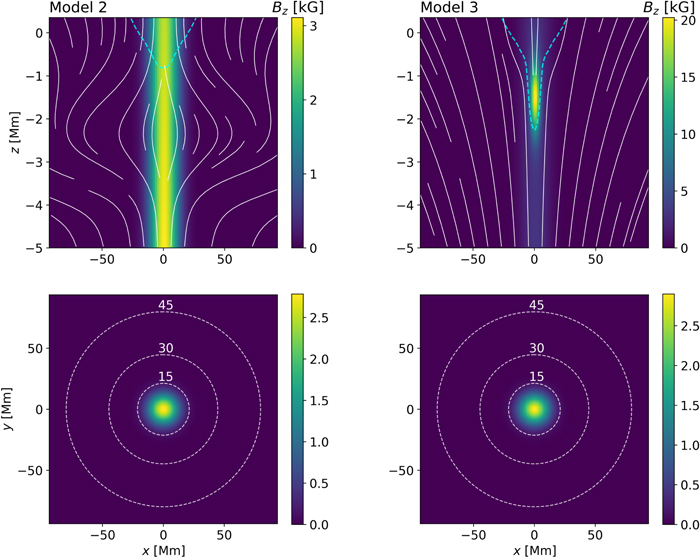
Figure 2. Flux tube "toy" models 2 and 3. The surface peak strength of the vertical magnetic field is 2.8 kG. A vertical slice is shown in the upper panels, a horizontal slice in the lower panels. White lines show the inclination, the cyan line depicts the layer where cA = cs. Note the vast changes of subsurface configurations compared to 1, but the very similar surface appearance. Not shown is the horizontal component of the magnetic field, causing model 2 to broaden at z = −2 Mm and model 3 to become more inclined at z = −1.5 Mm.
Download figure:
Standard image High-resolution image2.3. Mode Conversion and Downward Propagation
In order to keep the interactions at the flux tube boundary (that is cA = cs) as simple as possible, we employ a method similar to that of Shelyag et al. (2009). As mentioned before, only a single, quickly decaying oscillatory background displacement is used. It is quantified as:
where pt is the oscillation period, t0 is the starting time, σt is the temporal width (i.e., length),  is the location, and
  is the spatial width. We set pt = 302 s, equating to ≈3.31 mHz. Also t0 = 200 s, σt = 75 s (therefore quickly decaying),
  Mm (origin of the x–y-axis at the corner of the box), and
  Mm.
Mm.
This displacement will cause the propagation of a wave packet in every direction, simulated by SPARC. In Figure 3 this propagation is visualized. The left panels show snapshots of the full wave field vmagn where the upper panels show the y-component, and the lower panels the z-component. The simulation of the wave field seen in the left-hand lower panel corresponds to the (theoretical) propagation of a single wave packet on the solar surface. For the chosen time t = 30 minutes, the separation of multiple skip branches (see Section 3) already becomes visible. Note that there are some artificial features, such as absorption at the boundaries and amplitude distortion due to the Cartesian geometry, which is weak enough to be negligible. In the right panels, the instantaneous difference vdiff is shown.
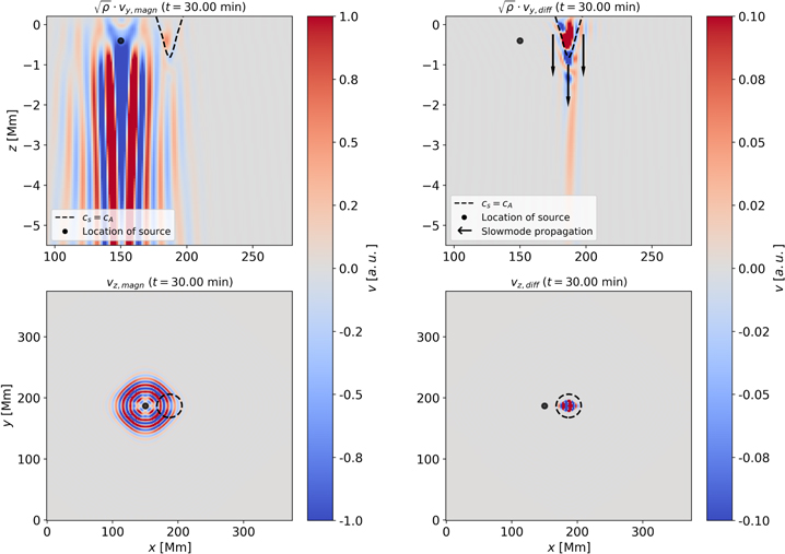
Figure 3. Wave propagation in the simulation box for vertical (top row) and horizontal (bottom row) cuts for t = 30 minutes. The left columns show the full wave field vmagn, caused by a wave packet originating from the location of the source (black dot). The right columns show the instantaneous difference vdiff, only depicting waves that are caused by the presence of the magnetic field. Upper panels showing vy are scaled with  . The cA = cs layer is shown as a black dashed line, black arrows indicate the predominant direction of wave propagation, after mode conversion at the cA = cs-layer. Note that the amplitude of vdiff is about 10% of the full wave field amplitude.
Download figure:
Standard image High-resolution imageWaves emerging from the source will behave as fast (fully) acoustic mode waves, once they cross the cA = cs layer, they can convert to the slow magnetoacoustic mode branch (Cally 2007). Slow mode waves will show two properties here: propagation preferably along magnetic field lines, and their transverse nature. Hence, showing the horizontal component will make these waves visible. As denoted in the top right panel of Figure 3 by black arrows, slow mode waves will start to trickle downwards along the flux tube, as long as they are within the cA = cs layer (and upwards out of the simulation domain). Once they cross that layer again, they can convert back to fast acoustic mode waves. These will now start to return to the surface after crossing their respective inner turning point, which is visualized in Figure 4 for t = 60 minutes and can best be seen for z < −5 Mm in the top right panel. Finally, the returning waves form a circular wave pattern centered on the flux tube, as seen in the bottom right panel of Figure 4.
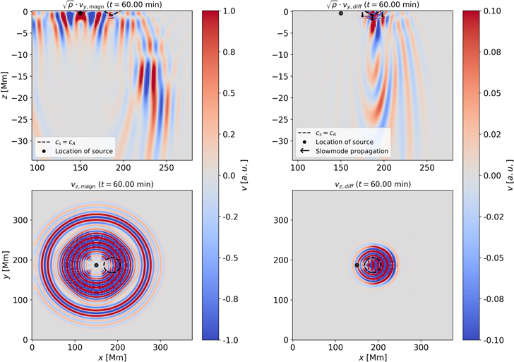
Figure 4. Same as Figure 3, but for t = 60 minutes. The upper panels show the whole depth of the simulation domain (other than Figure 3) with  and are scaled with
  . The initial wave packet has traveled through most of the atmosphere in this snapshot. Note the bending of the wavefronts (especially for vdiff) at large depths. This shows how the initially propagating wave turns back up toward the surface. The wave emergence in the lower right panel is delayed by approximately 16 minutes, which is the time it takes the initial wave packet to reach the center of the box, where the flux tube is located.
Download figure:
Standard image High-resolution imageTo summarize: waves that cross the flux tube boundary get partially converted and travel downwards, along field lines. They convert back again and travel to the surface. This is especially interesting, since the subsurface properties of the flux tube (at least within the cA = cs layer) will have an influence on the wave field that can be observed at the surface. Indeed we expect that the travel time, due to time being spent subsurface, and the shape, due to interference on the surface of the flux tube boundary, of the re-emerging wave packet will change. This change is thus related to the topology of the cA = cs layer. A quantitative analysis is done in the next section.
The surface signal vdiff as seen in the bottom right of Figure 5 is rather weak (about 10% of the full wave field amplitude), but is still contained in vmagn (as vmagn = vdiff + vquiet). It is however superimposed by the wave packet of the original source, making it difficult to detect. In Sections 3 and 4 it is shown how the two can be separated and potentially measured in real data.
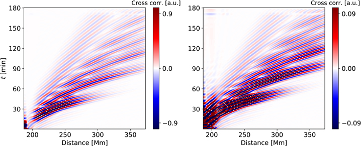
Figure 5. Time–distance diagrams for the single source analysis. Visible are branches of multiple skips for a frequency νsp of 3.3 mHz for the full wave field Cmagn (left) and the instantaneous difference Cdiff (right) as described in Equation (1). Correlation is done for a point in the center of the flux tube (at 186.88 Mm) from the full simulation to an arc trailing outwards in the full simulation (left) and the subtracted simulation (right). Color therefore denotes correlation strength in arbitrary units. Note that the amplitude for Cdiff is about 10% of the full wave field amplitude. No filter or averaging process is required for calculating the correlation, since only a single, isolated source is simulated.
Download figure:
Standard image High-resolution imageUsing the difference vdiff' we observe a similar wave pattern, but with an amplitude of about 1% of vmagn. From this behavior we learn that the re-emerging wave packet that is observed at the surface cannot only stem from thermal modifications to the background atmosphere (due to the presence of a magnetic flux tube), but must also carry contributions from the subsurface magnetic field itself. This is an important insight, meaning that vdiff is in fact sensitive to subsurface magnetic fields.
3. Time–Distance Analysis with Isolated Sources
The method we use to describe the wave propagation quantitatively is the time–distance analysis (Duvall et al. 1993; Gizon & Birch 2005). By cross-correlating the point x1 in which the single source is located, with an arc  at different times t and distances Δ, we can measure quantities like the group travel time tg, the amplitude A, and the central frequency ν0 of the propagating wave packet. For this analysis the source is now put in the center of the simulation box
  Mm, and thus x1 is put directly within the flux tube. This positioning eliminates the initial travel time delay, meaning that the wave packet will instantly interact with the magnetic field, making the analysis more simple. The cross-correlation
  calculated as a function of Δ is then shown in Figure 5. For the two simulation runs vmagn and vquiet we define:
where by difference, again the instantaneous difference  is meant. Note that the initial point x1 for the cross-correlation Cdiff is taken from the full wave field vmagn, since we want to analyze the correlation of the waves contained in vquiet with those of the initial displacement. Since the amplitude of vdiff is only about 10% of that of vmagn, it is expected that this is also the case for the amplitude of Cdiff, as can be seen in the right panel of Figure 5.
The broad contributions that can be seen for t > 90 minutes and Δ < 210 Mm can be assigned to a (unphysical but weak) reflection at the bottom boundary. Since these are restricted to an area that is generally not of interest, they can be ignored. Furthermore, the usual multiple skip branches are seen very clearly in both cases.
Again, we repeat this analysis with the subtraction of thermal runs, i.e., vtherm', in which we replaced the difference signal accordingly to calculate the correlation Cdiff. As expected, the main distinction is the amplitude. Due to the similarity of both correlation functions, we qualitatively conclude that Cdiff is in fact sensitive to the magnetic field.
As described in Section 2.3, the wave packet caused by the oscillatory background displacement will travel a certain distance (depending on the depth of the inner turning point) before re-emerging at the surface. It is therefore expected that the group travel times tg,magn of Cmagn and tg,diff of Cdiff differ. This can be measured by employing a fit to the data, to quantify the group travel times separately. For this, Gabor wavelets (Gizon & Birch 2005) of the form

are used. With A being the amplitude, dν the width and ν0 the central frequency of the spectral distribution of the wavelet, tg the group speed, and tp the phase speed. The results of  and
and  for this fit are shown for the first three branches in the left panel of Figure 6. A shift
  can clearly be seen for all branches and is highlighted with an annotation for the one-skip branch. Fitting the branches becomes more difficult starting from three-skip, since for such distances, multiple skips start to overlap. Since
  only varies slightly with the distance Δ, we estimate it by taking the average over Δ. This yields:

The same analysis for  and
and  gives similar results, but is less precise, since the fit does not converge as consistently and is generally less robust. We conclude that
  is the most accurate estimation of the time delay.
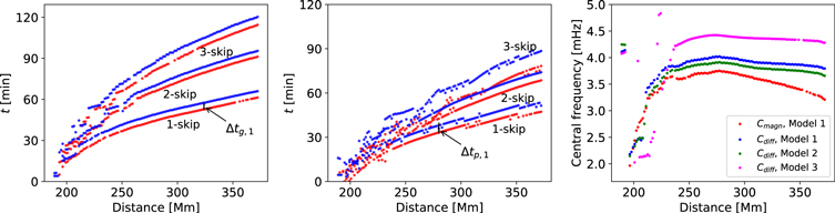
Figure 6. Results of fitting Gaussian wavelets to the different time–distance diagrams (as seen in Figure 5). Left: group travel times for the first three branches, for the full wave field  (red) and the instantaneous difference of the regular monolithic flux tube model
  (blue). Highlighted is also the very noticeable time delay of the group travel times for the first branch Δtg,1. Center: phase travel times, also with the time delay Δtp, 1. Right: central frequency ν0 in mHz of the fitted wavelet as a function of distance, for the full wave field (red), the regular monolithic flux tube model (model 1, blue), the alternative flux tube configuration (model 2, green), and the strongly modified model (model 3, magenta).
Download figure:
Standard image High-resolution imageShown in the center panels is the phase travel time tp. Here a similar behavior is observed, although the time delay

is more than twice as large as tg,1. However, the fit is much more erratic and becomes less reliable for small and large distances. For the analysis presented in the next section, we will be using tg,1 only, in principle it can nevertheless be performed with any quantity yielded by the fit.
Since one of the goals of this work is learning about the subsurface configuration of the simulated flux tube, this study is repeated for the other two flux tube models (see Figure 2). It turns out that changing the model affects Δtg only weakly. However, as shown in the right panel of Figure 6 other parameters like the central frequency ν0 (see Equation (2)) of the wavelet will show significant changes Δν0. While small changes in the model (model 1 to model 2) almost do not affect ν0 (Δν0 ≈ 0.04 mHz), more drastic changes (model 1 to model 3) may increase the frequency by up to Δν0 ≈ 0.5 mHz. This will allow us to distinguish different subsurface magnetic field configurations, as long as the signal Cdiff is available, or can be reconstructed reasonably well (more on this in Section 4).
The fact that the group travel time delay Δtg is similar for all three models can be explained by considering the radius of the cA = cs layer. Wave emergence visible in vdiff will start at the boundary of said layer, leading to similar subsurface travel times for similar radii r(z). When slow mode waves are converted back to fast mode acoustic waves at the boundary, interference between them happens, depending on the shape of the cA = cs layer. This interference will influence the wave pattern observed at the surface. That explains why ν0(Δ) (being an indicator for the spatial frequency distribution of the wave packet) is very similar for model 2 and the original model 1, but shows significant changes of up to 0.5 mHz for model 3, when the cA = cs-layer shape is changed drastically.
4. Analysis with More Realistic Simulations
Using real data, the instantaneous difference vdiff is generally not available. Any surface waves, that were caused by the mode conversion mechanism as described in Section 2.3 (seen in the right panels of Figure 4) are expected to be a feature of real sunspots as well. They will, however, have a small amplitude compared to other acoustic signals and will be swamped by them. In this section we will show one possible way to achieve a separation of the desired signal from the background nonetheless.
For this we ran two additional simulations with a solar-like stochastic forcing function, similar to the one described in Hanasoge (2007) again with and without magnetic field. Since the simulation does not include radiative transfer and the background is artificially stabilized, the resulting velocity fields will not exhibit granulation. Thus the simulation loses some degree of realism. For most acoustic analyses, however, granulation noise is unwanted anyway. The results are therefore treated as if granulation has been removed beforehand (by, for example, averaging or filtering processes). Looking again at the instantaneous difference vdiff, we see a circularly shaped wave pattern emerging from around the flux tube, equivalently to the behavior observed in Figure 4. Note that this is also briefly described in Hanasoge (2007).
We employ a time–distance analysis, similar to what we did in Section 3, considering the fact that the cross-correlation signal originating from within the flux tube Cdiff is delayed by the time Δtg. This time, however, the stochastic sources add a lot of unwanted contributions and noise. To still be able to construct a time–distance diagram, we employ a filtering process described in Gizon & Birch (2005) and rely on a point-to-arc average. A phase-speed filter that prefers waves with an average (one skip) travel distance of 14.5 Mm was applied. It is preferable to consider waves emerging close to the flux tube, since the amplitude of vdiff is higher, due to its circular nature. Furthermore, we use points in a circle with a radius of rC = 29.31 Mm around the flux tube (instead of directly inside it) to be correlated. Altogether, 616 point-to-arc cross-correlation functions are averaged.
As mentioned, the flux tube signal will be weak and superimposed by the cross-correlation signal of the original wave packet Cmagn, making it difficult to fit the desired signal Cdiff directly. The superposition will, however, modify the wave packet in an asymmetric way, since it only contributes at specific times (t + Δtg, no contribution at t − Δtg). This can be quantified by using the Gizon & Birch (2004) fitting method. It requires essentially only a reference function C0(t,Δ) that predicts the expected travel time at a certain distance Δ. In our case this function is easily obtained by using single source simulations as in Section 3. For real data one can either use theoretical predictions (i.e., the simulations done for this work, see Figure 5), or a cross-correlation function from heavily averaged time–distance diagrams. The result of this fitting method is given in Figure 7 at an exemplary distance Δ = 13.2 Mm, where the travel time tg,magn is annotated within the according image. A window with a width of  (shown as dashed orange line) was applied the interval of estimated travel time.
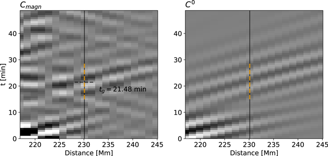
Figure 7. Cross-correlations of the full, multiple source wave field Cmagn (left) and the full, single source wave field (for the reference function) C0 (right) as a function of time t and distance. For both time–distance diagrams, a phase-speed filter was applied. For the left panel, an additional averaging process was applied. The right image appears smoother, since only a single source was simulated. The vertical black line marks the slice at which the fit was done, in this case Δ = 13.20 Mm (distance d = 230.13 Mm). The dashed orange line indicates the width of the window function. The dashed horizontal line and annotation show the fit result.
Download figure:
Standard image High-resolution imageThe challenge is now to detect a change in the travel time due to the emerging wave signal of the flux tube. We do this by "correcting" the data  , and the reference function
  . In principle the time–distance diagram on the right in Figure 7 exhibits contributions as shown on the right in Figure 5. This can be modeled, as long as we can estimate
  and the amplitude Adiff of the cross-correlation Cdiff with tg,Model and AModel. The actual cross-correlation functions for the full wave field Cmagn and instantaneous difference Cdiff differ in more than just the amplitude and travel time (see Figure 6, right panel), which is, however, neglected for the simplicity of this analysis. For the correction, we simply subtract the contribution of the flux tube:


where primed quantities means corrected. Correcting the data like this assumes that the difference signal vdiff contributes to the correlation Cmagn in a linear fashion. Generally the construction of Cmagn from vmagn and vdiff is more complicated, therefore the correction in Equation (6) is based on a first-order approximation. CModel is then constructed via

with, in this case,  . Fitting the corrected data
  will then yield a slightly modified travel time
  , shown in Figure 8. The difference for the two results
  is not equal to
  , as it is only a slight modification due to the contribution of the flux tube signal Cdiff. It is, however, related to Δtg, by how well the model attempt CModel agrees with Cdiff. An exemplary attempt at constructing the model CModel is shown in Figure 9. Generally it is expected that
  , since
  . Also, if CModel does not agree well with Cdiff, it is expected that
  . Summarizing, we can make the first constraint on the measurement of tg', and therefore for the agreement between CModel and Cdiff:

In our exemplary analysis, we find  , where we set (
 )
)  and
and  . Since for simulations, Cdiff is available, we can calculate the theoretical value of
  and deduce Δtg from fits, as shown in Figure 6, for comparison. Here we find:


As can be seen, the initial estimate of  leads to a
  that is already close to the theoretical value.
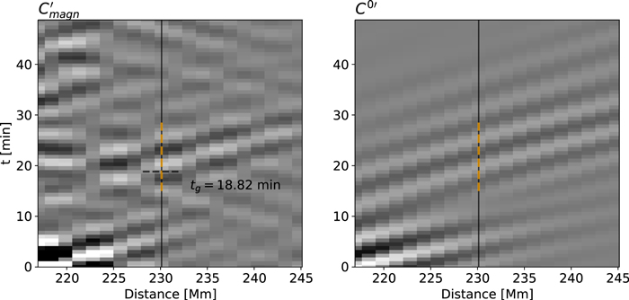
Figure 8. Same as Figure 7, except that primed quantities, i.e., time–distance diagrams where the correlation signal due to the presence of the magnetic field has been removed, are shown (as in Equation (6)). The travel time tg is decreased, due to the correction shown in Equation (6).
Download figure:
Standard image High-resolution imageThe constraint (8) yields a broad estimate on how to choose the parameters AModel and tg,Model for the model attempt CModel, but the exact value of Δtg will remain unknown for real data. One would need to do this analysis for several sunspots, to further narrow down Equation (8), or rely on the simulations done in this work, to have a reference for the required estimate of Δtg.
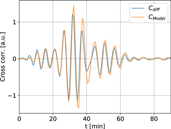
Figure 9. Desired (but in real data unknown) cross-correlation signal of Cdiff (blue) as a function of time t at a distance of Δ = 29.31 Mm (distance d = 246.24 Mm). Also plotted is the model attempt CModel (orange), constructed from the reference function C0 (see Equation (7)).
Download figure:
Standard image High-resolution image
5. Discussion
The mechanism of acoustic fast mode waves being converted into downward propagating slow mode waves is a known process (Cally et al. 2003; Rijs et al. 2015, 2016), but it has never been studied in particular. Moreover the ramping effect (Cally 2007), which is similar in its nature (upward propagation instead of the downward propagation considered here), was investigated more extensively, due to its possible contribution to acoustic halos. In this work, it was shown that flux tubes behave as sources of acoustic power, as long as they are being excited from the outside (Section 2.3). The consequence is that emerging waves from a sunspot contribute to the acoustic power in its vicinity. Of course, the absorption of p-mode power (Braun et al. 1987, 1988) makes detecting this power excess in real data nontrivial.
The time delay Δtg shown in Figure 6 is a way to distinguish the signals Cmagn and Cdiff. Setting up simulations with solar-like sources, it was shown that although the amplitude of the Cdiff is low, Δtg can still be estimated. As shown in Section 3 (left panel of Figure 6), a decent reconstruction of Cdiff via CModel using an estimate for Δtg may reveal subsurface properties of the investigated flux tube. It is necessary, however, to obtain the wave pattern of Cdiff to get dν and ν0 (see Equation (2)). Since tg does not vary for different flux tube models, dν and ν0 are needed to relate the surface signal to subsurface properties. It also appears that slight changes to the model that do not affect the cA = cs-layer do not affect the surface signal Cdiff. For real data this will require additional effort in creating CModel.
With the proposed method in Section 4, a measurement of  needs to be done reliably, which will be difficult in the case of real data. In principle, the method can be done for more sets of filters, as described in Gizon & Birch (2005) and thus, more distances Δ. We tested this here, and got similar results, but not for all distances Δ. This is expected, since, as mentioned, the amplitude of Cdiff becomes weaker for large Δ, decreasing the signal-to-noise ratio, due to its circular wave behavior. Again, another hurdle in estimating Δtg reliably.
6. Conclusion
Using the SPARC code to simulate the interaction of different kinds of waves with simple flux tube models, the effects of mode conversion have been visualized (see Figure 3). Slow mode waves traveling downwards along magnetic field lines of the flux tube convert back to acoustic fast mode waves, that deflect back up and are measurable at the surface. It is demonstrated how these surface waves are altered from subsurface changes in the flux tube model (see Figure 5). Moreover, the fact that these waves spend time traveling within the flux tube, a time delay Δtg (see Equation (3)) between re-emerging wave and original (as caused by the initial source) wave can be measured. We find that  . It was also found that subsurface changes in the flux tube models, especially changes to the shape of the cA = cs-layer, influence the frequency distribution of the surface wave pattern (see Figure 6).
A method to estimate Δtg for real data is presented in Section 4. Although the method might become unreliable for real data due to many sources of noise, for our simulations a value of  with an assumption of Δtg = 225 s proved to be accurate when compared to the theoretically predicted value of
  and the associated
  .
.
The reconstruction of CModel with quantities available in real data, in order to estimate Cdiff will need some additional effort, to be reliable. Also, measuring properties of the wave pattern, like the central frequency ν0, might require direct detection of Cdiff, which again will be difficult due to its comparatively low amplitude.
This work serves as a theoretical basis for a new method with the potential of adding to the knowledge of subsurface sunspot properties. The next step for further analysis regarding this topic is executing this study for real data and making these simulations more realistic by, for example, tuning the flux tube model, the background model etc. This will include fine tuning the proposed method as, for example, in Equation (8).
We thank Shravan M. Hanasoge for making the SPARC code, being the basis for this work, publicly available at http://www2.mps.mpg.de/projects/seismo/sparc/.