


Abstract
The Galactic stellar halo is predicted to have formed at least partially from the tidal disruption of accreted dwarf galaxies. This assembly history should be detectable in the orbital and chemical properties of stars. The H3 Survey is obtaining spectra for 200,000 stars and, when combined with Gaia data, is providing detailed orbital and chemical properties of Galactic halo stars. Unlike previous surveys of the halo, the H3 target selection is based solely on magnitude and Gaia parallax; the survey therefore provides a nearly unbiased view of the entire stellar halo at high latitudes. In this paper we present the distribution of stellar metallicities as a function of Galactocentric distance and orbital properties for a sample of 4232 kinematically selected halo giants to 100 kpc. The stellar halo is relatively metal-rich, ![$\langle [\mathrm{Fe}/{\rm{H}}]\rangle =-1.2$](https://content.cld.iop.org/journals/0004-637X/887/2/237/revision1/apjab5710ieqn1.gif) , and there is no discernible metallicity gradient over the range 6 < Rgal < 100 kpc. However, the halo metallicity distribution is highly structured, including distinct metal-rich and metal-poor components at Rgal < 10 kpc and Rgal > 30 kpc, respectively. The Sagittarius stream dominates the metallicity distribution at 20–40 kpc for stars on prograde orbits. The Gaia–Enceladus merger remnant dominates the metallicity distribution for radial orbits to ≈30 kpc. Metal-poor stars with [Fe/H] < −2 are a small population of the halo at all distances and orbital categories. We associate the "in situ" stellar halo with stars displaying thick disk chemistry on halo-like orbits; such stars are confined to
, and there is no discernible metallicity gradient over the range 6 < Rgal < 100 kpc. However, the halo metallicity distribution is highly structured, including distinct metal-rich and metal-poor components at Rgal < 10 kpc and Rgal > 30 kpc, respectively. The Sagittarius stream dominates the metallicity distribution at 20–40 kpc for stars on prograde orbits. The Gaia–Enceladus merger remnant dominates the metallicity distribution for radial orbits to ≈30 kpc. Metal-poor stars with [Fe/H] < −2 are a small population of the halo at all distances and orbital categories. We associate the "in situ" stellar halo with stars displaying thick disk chemistry on halo-like orbits; such stars are confined to  . The majority of the stellar halo is resolved into discrete features in chemical–orbital space, suggesting that the bulk of the stellar halo formed from the accretion and tidal disruption of dwarf galaxies. The relatively high metallicity of the halo derived in this work is a consequence of the unbiased selection function of halo stars and, in combination with the recent upward revision of the total stellar halo mass, implies a Galactic halo metallicity that is typical for its mass.
Export citation and abstract BibTeX RIS
1. Introduction
The stellar halo provides a unique window into the assembly history of our Galaxy. The long dynamical times imply that the halo has not undergone complete phase mixing, and therefore measurement of the orbital and chemical properties of halo stars should enable a reconstruction of the major events in the history of the Galaxy.
Early ideas concerning the formation of the stellar halo considered both "dissipative" (Eggen et al. 1962) and "dissipationless" (Searle & Zinn 1978) formation channels. In modern terminology these are referred to as "in situ" and "accretion" (or "ex situ") channels. In the former, halo stars are born within the Galaxy and are by some dynamical mechanism heated to halo-like orbits (e.g., Abadi et al. 2006; Zolotov et al. 2009; Purcell et al. 2010; Font et al. 2011; Cooper et al. 2015; Bonaca et al. 2017). In the latter, hierarchical assembly in a cold dark matter cosmology predicts that the halo was built at least in part by the tidal disruption of smaller dwarf galaxies (e.g., Johnston et al. 1996, 2008; Helmi & White 1999; Bullock & Johnston 2005; Cooper et al. 2010; Font et al. 2011).
In principle the combined orbital and chemical properties of stars should provide a powerful approach to understanding the origin of the halo. For example, such data should enable the categorization of in situ and accreted stars as a function of distance, metallicity, etc. A major goal is to identify the number of significant events that contributed to the accreted halo, estimate their progenitor masses and orbital properties, and ultimately reconstruct the build-up of the stellar halo. This field has a long and rich history of using the chemical–orbital properties of stars to study the origin of the halo (e.g., Sommer-Larsen & Zhen 1990; Ryan & Norris 1991; Majewski 1992; Zinn 1993; Carney et al. 1994; Chiba & Beers 2000; Carollo et al. 2007, 2010; Bell et al. 2008; Morrison et al. 2009; Bonaca et al. 2017; Belokurov et al. 2018; Helmi et al. 2018; Iorio & Belokurov 2019; Lancaster et al. 2019).
To date, nearly all observational work on the stellar halo has employed tracers that are biased with regard to metallicity. These biases ultimately stem from the fact that halo stars are rare and generally more metal-poor relative to the disk, combined with a desire to make efficient use of spectroscopic resources. Prior to Gaia, the most efficient way to separate halo from disk stars was to select stars with low metallicities. This bias can arise at two distinct stages in the analysis: first in the selection of targets for spectroscopic follow-up, and second via the identification of halo stars from the final sample. For example, the SDSS calibration stars used by Carollo et al. (2007, 2010) to study the stellar halo were selected on the basis of their blue colors. The SDSS SEGUE sample of K giants, which has been used to study the halo to great distances (e.g., Xue et al. 2015; Das & Binney 2016), was selected for spectroscopic follow-up on the basis of a complex set of color-cuts that favors low metallicities. Photometric metallicities of F/G turnoff stars are another popular method for studying the stellar halo. However, such samples are also constructed on the basis of color-cuts, and favor lower-metallicity stars (e.g., Ivezić et al. 2008; Sesar et al. 2011; Zuo et al. 2017). Rare populations such as RR Lyrae and blue horizontal branch stars are another popular tracer of the halo, in part because they are standard candles (e.g., Cohen et al. 2017; Iorio & Belokurov 2019; Lancaster et al. 2019). However, these populations also preferentially trace metal-poor stars. Biases incurred by using these populations to study the halo are very difficult to overcome without near-perfect knowledge of the underlying population and what fractions of stars were and were not included in the sample. These different observational methods have resulted in sometimes conflicting conclusions regarding the chemical–orbital structure of the stellar halo.
Thankfully, the observational landscape is rapidly improving on multiple fronts. Gaia has measured proper motions and parallaxes for over 1 billion stars to G ≈ 20 (Gaia Collaboration et al. 2018). The majority of halo stars are too distant to have precise parallaxes, and are too faint to have a measured Gaia radial velocity. To complement Gaia in the halo, we are undertaking the H3 Stellar Spectroscopic Survey of high-latitude fields (Conroy et al. 2019). The survey is delivering radial velocities, metallicities, and spectrophotometric distances for 200,000 parallax-selected stars. The key novelty of the H3 survey is a very simple selection function. H3 combined with Gaia is providing, for the first time, an unbiased view of the stellar halo to distances of 100 kpc.
In this paper we present the metallicity distribution of the stellar halo as a function of Galactocentric radius, vertical position (relative to the disk), and orbital properties. These results are used to understand the origin(s) of the Galactic stellar halo.
2. Data
The H3 Survey (Conroy et al. 2019) is collecting spectra for 200,000 stars in high-latitude fields. The survey footprint covers decl. > −20° and  . The selection function is very simple and consists of a magnitude limit of r < 18 and a parallax selection of π < 0.5 mas. Data collection began before Gaia DR2 was available, and so before the parallax selection could be made we obtained spectra for all stars with g − r < 1.0. A total of 19,300 stars were observed in this way (21% of the current sample). This color-cut is very mild—in the parallax-selected sample only 5% of stars have g − r > 1. None of the results presented below change if the early data are removed from the analysis.
The survey employs the medium-resolution Hectochelle spectrograph (Szentgyorgyi et al. 2011) on the MMT. Hectochelle uses a robotic fiber positioning system (Fabricant et al. 2005), enabling the placement of 240 fibers over a 1° diameter field of view (FOV). The instrument is configured to deliver R ≈ 23,000 spectra over the wavelength range 5150–5300 Å. As of 2019 June the survey has collected 89,000 spectra over 469 fields restricted to  . Details of the survey design and data quality can be found in Conroy et al. (2019).
Stellar parameters, including radial velocities, spectrophotometric distances, and abundances ([Fe/H] and [α/Fe]) are measured using the MINESweeper program (Cargile et al. 2019). The dominant α element in the H3 wavelength region is the Mg i triplet, so [α/Fe] is mostly tracing [Mg/Fe]. Briefly, MINESweeper combines spectral libraries and stellar isochrones to simultaneously fit for stellar parameters along with distance and redenning. Spectral libraries are computed by us using the ATLAS and SYNTHE programs (Kurucz 1970, 1993; Kurucz & Avrett 1981). We use the latest atomic line list from R. Kurucz (2019, private communication) and a comprehensive set of molecules including H2O, TiO, MgH, CH, CN, MgO, AlO, NaH, VO, FeH, H2, NH, C2, CO, OH, SiH, SiO, CrH, and CaH. The line list has been astrophysically calibrated against ultra-high-resolution spectra of the Sun and Arcturus. We use the MIST stellar evolution database for isochrones (Choi et al. 2016; Dotter 2016).
MINESweeper uses a Bayesian framework to fit the continuum-normalized spectrum and the broadband photometry (including Pan-STARRS, Gaia, 2MASS, WISE, and SDSS where available). Gaia parallaxes are used as a prior. Formal uncertainties on radial velocities determined from repeat observations are very small ( ). Derived distances have a typical formal uncertainty of ≈10% for giants. Uncertainties on [Fe/H] and [α/Fe] are ≈0.1 and ≈0.14 at S/N = 3 and ≈0.04 and ≈0.06 at S/N = 10. See Conroy et al. (2019) for further details of the measurement precision of derived parameters. Gaia DR2 proper motions for the H3 stars have median S/N of 25 and 33 for the R.A. and decl. components. For these two components, 86% and 91% of the sample have S/N > 5.
For calibration purposes the H3 Survey has obtained spectra of stars in the globular clusters M92, M3, M13, M71, and M107, and the open cluster M67. Together, these clusters span a range in metallicities from [Fe/H] = −2.3 to +0.0. Cargile et al. (2019) demonstrated that MINESweeper accurately determines distances, stellar parameters, metallicities, and abundances of the cluster stars. The literature values for most globular clusters show a scatter of ≈0.1 dex and MINESweeper often returns metallicities at the upper end of this range. These tests lead us to conclude that MINESweeper-derived metallicities are accurate to ≲0.1 dex. This issue is further discussed in Section 5.1 and Appendix A.
In this paper we use a high-quality subset of the full data set. Stars are selected that have a quality flag = 0 (removing bad data and very poor fits; ≈1% of the sample). We also place a limit on the median S/N across the H3 spectrum such that S/N > 3, which results in a higher-purity sample of metallicities. We remove the small number of blue horizontal branch stars that were explicitly targeted, since they have unreliable metallicities, and a small number of stars with very large tangential velocities (vT > 700 km s−1); visual inspection indicates that their stellar parameters are wrong and are therefore at incorrect distances. Giants with a derived rotational velocity >5 km s−1 are removed, as visual inspection indicates that these are dwarf stars being erroneously fit as a broadened giant. This affects 1% of the current sample and will be dealt with in a future version of the catalog by introducing a log g-dependent prior on the rotational broadening. These cuts leave 63,694 stars.
The spectrophotometric distances, radial velocities, and Gaia proper motions are then used to derive a variety of quantities including projections of the angular momentum vector onto the Galactocentric coordinate system (assuming the local standard of rest from Schönrich et al. 2010). Here we use the z-component of the angular momentum vector, Lz, as a way to group stars by their orbital properties (in our right-handed coordinate system, prograde stars have Lz < 0 and retrograde stars have Lz > 0).
We focus in this paper on kinematically selected halo giants. Specifically, we require  where V is the 3D velocity, and log g < 3.5. The kinematic selection efficiently removes stars on disk-like orbits (e.g., Venn et al. 2004; Nissen & Schuster 2010), and results in a sample of 14,152 stars. The giant selection ensures that the sample is not dominated by nearby halo dwarf stars, and results in a final sample of 4232 stars.
3. Test of the Selection Function with Mock Data
In this section we use a mock star catalog of the Galaxy in order to investigate the impact of our selection function on the inferred global properties of the halo.
Rybizki et al. (2018, R18) present a mock Galaxy tailored to Gaia-like data. The mock catalog is based on the Galaxia synthetic Galaxy (Sharma et al. 2011) and incorporates the major stellar components of the Galaxy including thin and thick disks, a bulge and a stellar halo. R18 adopt the Gaia DR2 error model for uncertainties on proper motions and include a realistic 3D dust extinction map.
The default stellar halo is uniformly old (13 Gyr) and has a metallicity distribution function (MDF) that is Gaussian with a mean of [Fe/H] = −1.78, a dispersion of σ[Fe/H] = 0.5, and no gradient with Galactocentric radius. We have also explored a modified mock catalog in which the stellar halo has a metallicity gradient that is linear in log(Rgal) from [Fe/H] = −1.2 to [Fe/H] = −2.0 over the range 10–100 kpc. The profile is flat at <10 kpc and >100 kpc. We have recomputed photometry self-consistently for both versions of the mock catalog using the MIST isochrones and bolometric correlations (Choi et al. 2016).
We have taken the R18 mock and made several modifications in order to approximate the H3 Survey data. We impose the H3 selection function (r < 18 and π < 0.5 mas) and the H3 window function (keeping only stars that lie within the FOV of our observations). After applying the selection function, we randomly select a maximum of 200 stars within each FOV, as only ≈200 stars are assigned fibers per pointing. We then apply the same kinematic halo selection as discussed in Section 2 and select giants with log g < 3.5. Finally, we impose a 10% fractional uncertainty on the distances. This is the median distance uncertainty for the giants in H3 (Conroy et al. 2019).
With these H3-like mock catalogs we are now in a position to assess the H3 selection function on the metallicity profile in the halo. The H3 selection function is very simple, but one could imagine that even a magnitude selection might result in a bias owing to the fact that the most luminous giants are brighter in the r-band at lower metallicities.
We test this effect in Figure 1, which shows the distribution of metallicities versus radius for the kinematically selected halo giants in the two versions of the R18 mock catalog. The top panel shows the default R18 stellar halo metallicity model: a flat profile in radius. The bottom panel shows the model that has a gradient from 10 to 100 kpc. Median metallicities and 1σ scatter values are computed in radial bins (points with error bars), and compared to the true underlying distribution (solid and dotted lines). The excellent agreement implies that the H3 selection function does not impart a bias in the recovered metallicity gradient.

Figure 1. Effect of the H3 selection function on the recovered metallicity profile in the halo. Top and bottom panels show two models for the input metallicity profile of the R18 mock stellar halo. Small points show the metallicities of kinematically selected halo stars drawn from the R18 mock catalog subject to the H3 selection function (r < 18, π < 0.5) and the H3 window function. Large open symbols and errors show the median and standard deviation in radial bins. Solid and dashed lines show the true input metallicity distribution of the R18 halo (mean and scatter) for the two model metallicity profiles. Agreement between the open symbols and lines indicates that the H3 selection function does not impose a metallicity bias as a function of radius.
Download figure:
Standard image High-resolution image4. Results
4.1. The Halo Metallicity Profile
We begin with an overview of the abundance patterns of the kinematically selected halo giants. Figure 2 shows [α/Fe] versus [Fe/H] for the main sample (top panel), and for a high-S/N subset (bottom panel). There are several distinct populations in this diagram, though we draw attention to the stars above the dashed line. These stars have thick disk chemistry and yet are on halo-like orbits. We identify such stars with the "in situ" stellar halo and discuss their location in various diagrams below. This population has been identified in previous work (e.g., Bonaca et al. 2017; Di Matteo et al. 2019; Haywood et al. 2018; Belokurov et al. 2019), and is often interpreted as stars born within the early Galaxy that have been heated, e.g., by a major merger, to halo-like orbits.

Figure 2. [α/Fe] vs. [Fe/H] for kinematically selected halo giants in the H3 Survey. The top panel shows the fiducial sample with spectral S/N > 3. In the bottom panel we show a subset of the data with S/N > 10 where the various subpopulations are even more clearly visible. Stars above the dashed line have thick disk chemistry and so are associated with the in situ stellar halo. Median uncertainties are shown in the lower left corner of each panel.
Download figure:
Standard image High-resolution imageFigure 3 shows the metallicity profile of kinematically selected halo giants from the H3 Survey as a function of distance from the Galactic plane (top panel) and Galactocentric radius (bottom panel). In the bottom panel we also show median metallicities and 1σ scatter in radial bins. The median metallicity of the entire sample is ![$\langle [\mathrm{Fe}/{\rm{H}}]\rangle =-1.2$](https://content.cld.iop.org/journals/0004-637X/887/2/237/revision1/apjab5710ieqn7.gif) and is shown as a solid line. Stars with thick disk chemistry are shown as gray points.
and is shown as a solid line. Stars with thick disk chemistry are shown as gray points.

Figure 3. Stellar metallicity vs. distance from the Galactic plane (top panel) and Galactocentric radius (bottom panel) for kinematically selected halo stars from the H3 Survey. Gray points have thick disk chemistry as defined in Figure 2 and are therefore defined as the in situ stellar halo. In the bottom panel, the mean and scatter is shown in blue as a function of radius. The overall profile is remarkably flat with ![$\langle [\mathrm{Fe}/{\rm{H}}]\rangle =-1.2$](https://content.cld.iop.org/journals/0004-637X/887/2/237/revision1/apjab5710ieqn8.gif) , although there are clearly multiple distinct populations. The median measurement uncertainty on [Fe/H] is 0.05 dex.
, although there are clearly multiple distinct populations. The median measurement uncertainty on [Fe/H] is 0.05 dex.
Download figure:
Standard image High-resolution imageThere are several important features in Figure 3. The overall metallicity profile is remarkably flat across the entire range from ≈6–100 kpc. There is marginal evidence for a lower mean metallicity beyond ≈50 kpc, but there are too few stars in the current data to draw strong conclusions. Importantly, the average metallicity is considerably more metal-rich than most previous work. We return to this point in Section 5. There are two populations that are more metal-rich than the rest of the halo. The first is at  and is associated with the in situ halo (i.e., stars having thick disk-like chemistry). The second metal-rich component is at 20 ≲ Rgal ≲ 40 kpc and is associated with the Sagittarius stream. Finally, there is a clear metal-poor component ([Fe/H] ≲ −2) that extends to ≈100 kpc.
The MDF is shown in Figure 4 in three radial bins. At Rgal < 10 kpc one clearly sees evidence for two distinct populations, including a main population with a mean metallicity of [Fe/H] = −1.2 and a secondary metal-rich population. Removing stars belonging to the in situ halo as defined in Figure 2 results in an MDF with a single peak at [Fe/H] = −1.2, shown as the thin line in Figure 4.

Figure 4. Metallicity distribution functions (MDFs) in three radial bins for kinematically selected halo giants. The gray dotted line is an analytic chemical evolution model fit to the distribution in the middle panel. In the left panel, we also show the MDF excluding the in situ halo stars (thin solid line labeled "accreted"), while in the right panel we show the MDF excluding Sagittarius stream stars. In the left and right panels the dotted line is scaled to the number of stars in the accreted and non-Sgr components, respectively. The bin width used to compute the histograms is 0.1 dex.
Download figure:
Standard image High-resolution imageAt 10 < Rgal < 30 kpc the distribution is consistent with a single population with a mean metallicity of [Fe/H] = −1.2. To explore this further, we fit the MDF with a simple chemical evolution model. Kirby et al. (2011) modeled the MDFs of a sample of dwarf galaxies using a variety of simple chemical evolution models. They found that the "best accretion model" of Lynden-Bell (1975) overall performed well in reproducing the observed MDFs. In this model the gas mass has a non-linear dependence on the stellar mass, quantified by the parameter M which is the ratio between the final and initial mass of the system. We use this model and fit its two free parameters (the yield, p = 0.08, and M = 2.1) to the data in the middle panel of Figure 4. The result is shown as a dotted line, and is a good fit to the observed MDF, suggesting that one population dominates this radial range.
In the third panel of Figure 4 we show the MDF for 30 < Rgal < 100 kpc. There are at least two distinct populations based on the MDF alone: a metal-rich population at [Fe/H] ≈ −1 and a metal-poor population at [Fe/H] ≈ −2.1. We have identified stars likely belonging to the Sagittarius stream according to their distribution in Ly − Lz space. Specifically, stars with Ly < −Lz − 3 × 10³ kpc km s−1 are selected as Sagittarius stars (see B. D. Johnson et al. 2019, in preparation, for details). Removing these stars from the MDF results in the thin line in Figure 4. Even after removing Sagittarius there are clearly at least two distinct chemical populations.
4.2. Halo Metallicities versus Orbital Properties
In this section we investigate the dependence of halo metallicities on orbital properties. In particular, we focus on the z-component of the orbital angular momentum, Lz, and we define three groupings of stars: prograde (Lz < −5 × 10² kpc km s−1), retrograde (Lz > 10 × 102 kpc km s−1), and radial orbits (−5 × 10² < Lz < 10 × 102 kpc km s−1). The quantitative selection was chosen based on the distribution of stars in E − Lz space, where E is the total energy of the orbit (the distribution of H3 stars in E − Lz will be presented in R. P. Naidu et al. 2019, in preparation). As shown in previous work (e.g., Belokurov et al. 2018; Helmi et al. 2018) and with H3 data in R. P. Naidu et al. (2019, in preparation), there is a population of stars on strongly radial orbits that cluster in the radial orbit selection region we have outlined. This population has been referred to in the literature as Gaia–Enceladus (Helmi et al. 2018) and the Gaia–Sausage (Belokurov et al. 2018), with slight differences in how the population is defined in each case. There is a slight asymmetry in the distribution, which led us to impose an asymmetric selection in Lz.
In Figure 5 we show the metallicities of kinematically selected halo giants as a function of orbital properties. In the top panels we show [Fe/H] versus Galactocentric radius and in the bottom panels we show [Fe/H] versus [α/Fe].

Figure 5. Top panels: metallicity vs. Galactocentric radius separated according to the z-component of the angular momentum (prograde, radial, and retrograde in the left, middle, and right panels). Bottom panels: distribution of stars in [α/Fe] vs. [Fe/H]. Only kinematically selected halo stars are shown. Gray points lie above the dashed lines in the bottom panels and mark the in situ halo stars. The Sagittarius stream is prominent in the left panels. The Gaia–Enceladus remnant dominates the middle panels along with a metal-rich, α-rich population of in situ stars. The right panels is perhaps dominated by the Sequoia remnant. In the lower panels, the red star marks the median values of [Fe/H] and [α/Fe] for the accreted stars (black points).
Download figure:
Standard image High-resolution imageThe top panels display a wealth of structure. The prograde-halo population is dominated by a relatively metal-rich feature at 20 < Rgal < 40 kpc. This is the Sagittarius stream, and will be discussed in detail in B. D. Johnson et al. (2019, in preparation). There is also a distinct metal-poor population at [Fe/H] ≈ −2. The radial-halo population is composed of two principal populations. The dominant population is at [Fe/H] ≈ −1.2 and extends to ≈30 kpc. This is the Gaia–Enceladus merger remnant. There is also a metal-rich ([Fe/H] > −1) population confined to Rgal ≲ 20 kpc ( gray points) which we associate with the in situ halo. The retrograde-halo population is on average more metal-poor than the other two orbital groupings. There is a population at [Fe/H] ≈ −1.2 that clearly has a more extended distribution in Galactocentric radius compared to the halo stars on radial orbits. In addition, there is a relatively prominent metal-poor population that is also quite extended in radius.
In the bottom panels of Figure 5 one sees systematic variation in [α/Fe] with orbital properties. The prograde halo (dominated by the Sagittarius stream) is relatively α-poor; the radial group (dominated by Gaia–Enceladus) is more α-rich, while the retrograde group is the most α-rich and metal-poor.
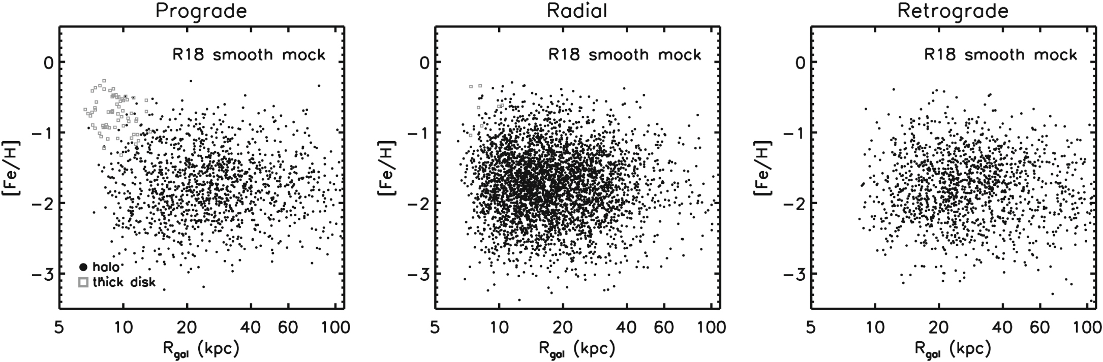
In Figure 6 we show the metallicity distributions of kinematically selected halo stars separated by orbital properties for the fiducial R18 smooth mock catalog. As a reminder, this mock catalog was generated assuming intrinsically smooth distributions of the thin and thick disks and a single-component smooth stellar halo. The mock data set has the H3 selection function applied and a realistic error model for all relevant parameters. True halo stars are shown as black symbols, while thick disk stars are shown in gray. As expected, the distribution of stars in Figure 6 is smooth, and there is no discernible orbital dependence of the halo population. Within the prograde group there is small population of thick disk stars at Rgal < 10 kpc. This population is not a consequence of the error model in the mock data but instead seems to simply be the tail of the thick disk distribution. Note that thick disk stars are not present in significant numbers among the radial orbit group, in contrast to the data.

Figure 6. As in Figure 5, now showing kinematically selected halo stars from the R18 smooth mock catalog. Black points indicate true halo stars while gray points belong to the thick disk. In this model the halo population is intrinsically smooth with a power-law density profile and a flat metallicity profile. The presence of gray points in the left panel means that thick disk stars are entering into the kinematic halo selection. These stars are not present in significant numbers among the radial orbits (middle panel), in stark contrast to the data (Figure 5, middle panel).
Download figure:
Standard image High-resolution imageFigure 7 shows the MDF of kinematically selected halo giants in the three orbital groups. In this figure we have removed the metal-rich and α-rich stars (the in situ stars) that lie above the dashed lines in the lower panels of Figure 5. The dotted line is the best accretion chemical model fit to the data in the middle panel, and reproduced in the other panels for comparison purposes. The MDFs in Figure 7 add support to the interpretation of Figure 5 discussed above. In particular, the prograde and retrograde groups clearly show at least two distinct populations (even after removing the in situ component), while the radial group appears to be dominated by a single population.

Figure 7. Metallicity distribution functions (MDFs) of H3 stars shown for prograde, radial, and retrograde orbits. Here we have removed the in situ halo stars (those above the dashed lines in the lower panels of Figure 5). The dotted line is a simple chemical evolution model fit to the MDF in the middle panel and replicated in other panels for comparison purposes. There are multiple chemically distinct stellar populations among the prograde and retrograde stars. The population of stars on radial orbits are consistent with arising from a single stellar population.
Download figure:
Standard image High-resolution imageIn Figure 8 we show the distribution of halo stars in Lz versus [Fe/H]. The H3 sample is grouped into three radial bins: Rgal < 10 kpc, 10 < Rgal < 30 kpc, and 30 < Rgal < 100 kpc. We also mark in gray the in situ halo stars. Note that stars at greater distances naturally occupy a wider range in Lz values, which explains why stars at smaller Rgal are confined to a relatively narrow range in Lz.
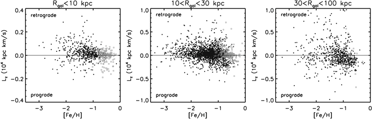
Figure 8. Lz vs. [Fe/H] for kinematically selected halo giants from the H3 Survey. Stars are grouped in three radial bins: Rgal < 10 kpc, 10 < Rgal < 30 kpc, and 30 < Rgal < 100 kpc. Grey points mark the in situ halo stars defined in the bottom panels of Figure 5.
Download figure:
Standard image High-resolution imageThere are multiple distinct populations evident in Figure 8. The Sagittarius stream comprises the prograde metal-rich region, while the Gaia–Enceladus remnant dominates the radial Lz ∼ 0 region for Rgal < 30 kpc. At [Fe/H] < −2 there is a strongly retrograde population at Rgal < 30 kpc; the nature of the metal-poor population at greater distances is unclear. Finally, there is a hint of a retrograde population at −2 < [Fe/H] < −1, which may be associated with the Sequoia merger event (Matsuno et al. 2019; Myeong et al. 2019).
5. Discussion
5.1. Caveats and Limitations
The stellar parameter pipeline MINESweeper contains several important limitations, including the use of solar-scaled isochrones and a fixed microturbulent velocity. In order to test the effect of these and other limitations and assumptions, in Cargile et al. (2019) we validated the H3 pipeline in several ways. These included running the H3 pipeline on data for several star clusters spanning the range [Fe/H] = −2.2 to [Fe/H] = +0.0. The derived metallicities and [α/Fe] values were in good agreement with literature estimates. However, in some cases the derived metallicities were 0.05–0.1 dex higher than previous work. It is possible that our overall metallicity scale is therefore slightly too high, though the magnitude of the effect is likely less than 0.1 dex. We explore this issue further in Appendix A, where H3 metallicities are compared to APOGEE, LAMOST, and SEGUE metallicities for stars in common between the surveys.
The current H3 footprint is restricted to  with many more fields in the Northern Hemisphere (Conroy et al. 2019). Upon completion of the survey the footprint will sparsely cover ≈35% of the sky. A full accounting of the stellar halo must take the survey footprint into account. For example, structure that is confined near the disk plane will be missed in a high-latitude survey. Special care must also be given to halo structure that is at least somewhat coherent on the sky (such as Sagittarius). We have not attempted any such corrections in the present work, so quantitative determination of the mass fraction in various halo structures must be viewed as preliminary.
Finally, we caution that our spectroscopic survey is able to detect as coherent structures in phase space only those systems that had a relatively high progenitor stellar mass. We can estimate a rough mass limit as follows. The H3 Survey has covered 370 sq. deg. to date, which represents ≈1% of the sky. We have focused here on giants with log g < 3.5. Such stars comprise ≈0.3% of the stars in an old stellar population (estimated from the MIST isochrones assuming a Kroupa initial mass function; Choi et al. 2016). If we optimistically assume that we have obtained a spectrum for every giant within each field of view, then our sampling rate is approximately 1:300,000. This number can be estimated another way: if we assume that there are ≈109 stars in the stellar halo (Deason et al. 2019), and our current sample of halo giants contains 4232 stars, then the sampling rate is 1:250,000—reasonably close to the previous estimate. If one assumes that 100 stars are required in order to identify a cold feature in phase space, then our sensitivity limit is in the range of M* ≈ 3 × 10⁷ M⊙. In detail, this limit will be lower for systems that disrupted nearer to the solar neighborhood compared to more distant systems. This is due to the fact that our magnitude limit corresponds to relatively more luminous stars at greater distances, and such stars are an intrinsically smaller fraction of the underlying population. The main point is that any survey of the halo will only be sensitive to disrupted systems above a certain mass threshold, and this threshold must be taken into account when interpreting the results.
5.2. Comparison to Previous Work
There is a large body of work exploring the metallicity and orbital properties of the stellar halo. When comparing to previous work, several issues must be kept in mind. (1) The selection of stars entering the spectroscopic catalog frequently is strongly biased toward a particular stellar population. For example, spectra for Sagittarius stream stars have often been obtained for stars satisfying the M giant color-cuts of Majewski et al. (2003). Such a selection favors more metal-rich populations. Other samples such as SDSS SEGUE spectra, favor metal-poor populations (see Appendix B below). (2) The definition of "halo" varies from author to author. In many cases metallicity alone is used to define the halo. (3) The volume probed can vary dramatically, from samples encompassing the very local halo (e.g., within 1 kpc of the Sun), to sparse tracers such as RR Lyrae stars that provide a view of the entire stellar halo.
Carollo et al. (2007, 2010) used SDSS spectrophotometric calibration stars to study the metallicity and orbital properties of the local halo (d < 4 kpc). These stars were selected to have blue colors, and therefore are strongly biased toward low metallicities, as noted by the authors. They identify two components to the stellar halo (which they refer to as the "dual halo"): a metal-rich ([Fe/H] = −1.6) inner halo with highly eccentric orbits, and a metal-poor ([Fe/H] = −2.2) retrograde outer halo. The transition between these two components occurs around Rgal ≈ 20 kpc (the authors were able to infer the properties of the halo beyond their d < 4 kpc selection by considering the maximum vertical extent of stars throughout their orbits). These authors fit multi-component Gaussians to the MDFs in order to isolate various components. We caution that such a procedure can be difficult to interpret since MDFs for single populations are expected on theoretical grounds to have a strong skew toward low metallicities (e.g., closed box and other, more realistic, chemical evolution models; see Section 4.1). In agreement with Carollo et al., we find that within ∼30 kpc the stellar halo is dominated by a single population with highly radial orbits (referred to as Gaia–Enceladus, or Gaia–Sausage in the recent literature; Belokurov et al. 2018; Helmi et al. 2018).
However, in contrast with Carollo et al. (2010), at no distance or orbital category do metal-poor stars (e.g., [Fe/H] < −2) dominate the population. We speculate that this difference is due to the fact that Carollo et al. analyze stars within 4 kpc in order to infer the properties of the halo at greater distances. Any populations at large distances that possess appreciable angular momentum will not be well represented in a local sample (the most striking example of this is the Sagittarius stream, although the Sequoia remnant also possesses a significant amount of angular momentum).
Liu et al. (2018) use LAMOST spectra to study the MDF of A/F/G/K-type stars with  . By fitting Gaussians to the MDF, they identify three distinct components with peaks of −0.6, −1.2 and −2.0; the first they identify as the thick disk, and the last two as the inner and outer halo. They show that the thick disk component is confined to
  , in broad agreement with our results. They also find that the retrograde stars are on average more metal-poor than the prograde stars, also in agreement with our results.
Several studies have analyzed the global metallicity gradient of the stellar halo. Both Xue et al. (2015) and Das & Binney (2016) used SEGUE K giants to measure the metallicity gradient to ≈100 kpc. They define halo stars via a metallicity cut ([Fe/H] < −1.2 and [Fe/H] < −1.4, respectively). Both authors find evidence for a shallow (but non-zero) metallicity gradient such that the metallicity decreases by ≈0.1–0.2 dex from 10 to 100 kpc. In contrast, we find no evidence for a metallicity gradient over the interval ≈6–80 kpc. The differences are likely due to the metallicity cuts imposed in the definition of the halo samples in Xue et al. (2015) and Das & Binney (2016). Fernández-Alvar et al. (2017) use APOGEE data to study the halo metallicity profile. They focus on stars with  that satisfy a kinematic halo selection similar to what we employ. They find a flat gradient over the range 10 ≲ Rgal ≲ 30 kpc, in agreement with the results presented here.
Xue et al. (2015) estimate a mean metallicity of the halo of [Fe/H] = −1.7, which is considerably more metal-poor than our value (−1.2). There are several reasons for this discrepancy. First, Xue et al. define halo stars according to [Fe/H] < −1.2. Second, the metallicity scale of SEGUE appears to be slightly lower than H3 (see Appendix A). Third, the color selection used in the SEGUE K giant sample excludes metal-rich stars (see Appendix B).
Recently, Mackereth et al. (2019) used APOGEE data to isolate highly eccentric stars on halo orbits and report an MDF that peaks at [Fe/H] ≈ −1.3. They caution that the APOGEE selection function makes it difficult to interpret the overall shape of the MDF. Nonetheless, their MDF is in good agreement with our results.
In general, while there is broad agreement in the literature on the main characteristics of the stellar halo, it is often difficult to make quantitative comparisons owing to the fact that most previous work has relied on metallicity-biased tracers of the halo, and/or has focused on a small volume centered on the solar neighborhood.
5.3. The Origin of the Stellar Halo
A basic prediction of cold dark matter cosmology is the hierarchical assembly of galaxies and their stellar halos (e.g., Johnston et al. 1996; Helmi & White 1999; Bullock & Johnston 2005). Evidence for the tidal disruption of smaller dwarf galaxies is now ubiquitous both in our Galaxy (e.g., Majewski et al. 2003) and beyond (e.g., Ibata et al. 2001). Attempts to provide objective measures of the degree of structure in the halo have found good agreement with cosmological models (Bell et al. 2008).
With a high-quality, unbiased sample of 4232 giants with well-measured distances, proper motions, metallicities, and abundances extending from 6 to 100 kpc, we are in a position to provide a holistic view of the stellar halo. This view is provisional for the reasons mentioned in Section 5.1, and will be updated as additional data are collected.
The stellar halo beyond  is overwhelmingly of accreted origin. We identified a population of stars with thick disk chemistry that we associate with the in situ halo. Such stars comprise ≈25% of the halo at 6 ≲ Rgal ≲ 10 kpc, and only a few percent at greater distances. Our data do not probe halo stars at Rgal < 6 kpc so it is possible that in situ halo stars comprise a greater fraction of the halo nearer to the Galactic center. These results are in broad agreement with predicted in situ halo fractions from the hydrodynamical simulations of Zolotov et al. (2009), who predicted a large fraction on in situ stars confined to the inner regions of their simulated galaxies. These results confirm and extend previous analysis of Gaia DR1 data of the local stellar halo (within 3 kpc of the Sun) by Bonaca et al. (2017), and analysis of Gaia DR2 data by Haywood et al. (2018), Di Matteo et al. (2019), and Belokurov et al. (2019). These authors identified a population of stars on halo orbits with thick disk chemistry that they identified as the in situ stellar halo. These stars are believed to have formed within the Galaxy, e.g., as an early disk population, and were subsequently heated to halo-like orbits, perhaps as the result of a major merger.
Previous work has identified at least four major chemical–orbital structures in the halo: Gaia–Enceladus/Gaia–Sausage (Belokurov et al. 2018; Helmi et al. 2018), Sequoia (Myeong et al. 2019), Sagittarius (Majewski et al. 2003), and a metal-poor retrograde component (Carollo et al. 2007; Helmi et al. 2017). These four components are clearly visible in our data. The first three have remarkably similar average metallicities (in the range −1.0 to −1.3), which helps to explain the very flat metallicity gradient from 6 to 100 kpc in spite of the fact that different components dominate in different radial ranges. The mass–metallicity relation at z = 0 has a slope of 0.3 dex (Kirby et al. 2013) and the dominant three components of the Milky Way (MW) halo have estimated stellar masses that differ by a factor of 10–100. One might therefore have expected a larger range in metallicities. However, the mass–metallicity relation is believed to evolve with redshift, such that the zero-point decreases with increasing redshift (e.g., Zahid et al. 2013; Ma et al. 2016). If the more massive systems accreted earlier, then the evolving mass–metallicity relation would result in a small range in metallicities among the major remnants in the halo.
The nature of the metal-poor component ([Fe/H] < −2) is difficult to discern based on the analysis presented here. This population is clearly distinct from the more metal-rich stars at Rgal > 30 kpc. Such stars are also present in appreciable numbers at Rgal < 30 kpc, and while they are not an obviously distinct population based on metallicities alone, they do appear to occupy distinct regions of orbital parameter space. We conjecture that the metal-poor component may in fact be tracing multiple distinct populations. This issue is discussed further in C. J. Carter et al. (2019, in preparation).
In summary, the data strongly favor a multi-component stellar halo comprised primarily of accreted stars from at least four distinct progenitor systems. We expect additional structures to be identified as new data allow sensitivity to lower-mass progenitor systems.
5.4. The Galactic Stellar Halo in Context
Several authors have explored the correlation between stellar halo mass and metallicity both in observations and simulations. Deason et al. (2016) developed a semi-empirical model that predicted a strong correlation between stellar halo mass and metallicity. In their model, this relation is set by the hierarchical assembly of dark matter halos in conjunction with an empircally constrained, redshift-dependent stellar mass–halo mass relation and an empirical mass–metallicity relation. D'Souza & Bell (2018) and Monachesi et al. (2019) presented similar correlations based on the Illustris and Auriga hydrodynamical simulations. These authors compared their models to observations of the stellar halos of the MW, M31, and six galaxies from the GHOSTS Survey (Harmsen et al. 2017).
The consensus from these comparisons is that the MW stellar halo has a metallicity lower than expected for its mass. In these comparisons a stellar halo metallicity of −1.6 to −1.7 was adopted, along with a stellar halo mass of 0.5 × 10⁹ M⊙. Recently Deason et al. (2019) used Gaia data to revise the stellar mass in the MW halo significantly upward. This revision results in a MW stellar halo that is even more discrepant with the observed stellar mass–metallicity relation defined by other galaxies.
One of the key results of our work is the higher average metallicity of the Galactic stellar halo compared to previous work. We therefore revisit this issue in Figure 9, where we plot the total stellar halo mass as a function of halo metallicity. For the MW, we adopt our average metallicity of −1.2, and the updated halo mass from Deason et al. (2019). The Deason et al. stellar halo mass depends on the assumed metallicity of the halo; adopting our mean value of [Fe/H] = −1.2 results in a stellar halo mass of (1.05 ± 0.25) × 109 M⊙. The GHOSTS data are from Harmsen et al. (2017), where the metallicities are quoted at 30 kpc. The M31 stellar halo mass is adopted from Harmsen et al. (2017), which is in turn based on Ibata et al. (2014). For the halo metallicity of M31 at 30 kpc, we follow D'Souza & Bell (2018) and adopt [Fe/H] = −0.5. We also include older estimates for the MW stellar halo mass (Bland-Hawthorn & Gerhard 2016) and metallicity (Xue et al. 2015).
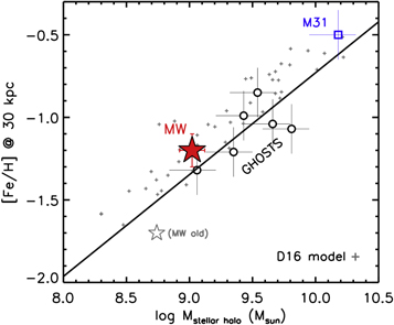
Figure 9. Total stellar halo mass vs. stellar halo metallicity. The metallicity is quoted at a common Galactocentric distance of 30 kpc (although note that the MW gradient is flat so the choice of reference point will not change the location of the MW in this diagram). The MW metallicity is from the present analysis and the adopted stellar halo mass is from Deason et al. (2019). We also show the previous canonical values for the MW halo as a gray star. GHOSTS data are from Harmsen et al. (2017) and the sources of the M31 data are described in the text. Small gray symbols are predictions from the semi-empirical model of Deason et al. (2016) and the solid line is a linear fit to the combined GHOSTS+M31+MW data.
Download figure:
Standard image High-resolution imageThe revised stellar mass and metallicity of the halo places the Galaxy on the locus defined by other galaxies. NGC 4565 from the GHOSTS Survey has a halo most closely resembling that of the Galaxy. Harmsen et al. (2017) quotes a total stellar mass for NGC 4565 of (8 ± 2) × 1010 M⊙, in broad agreement with modern estimates of the total stellar mass of the Galaxy of (5−6) × 1010 M⊙ (Licquia & Newman 2015; Bland-Hawthorn & Gerhard 2016). NGC 4565, an edge-on spiral galaxy, may therefore be a useful MW analog.
6. Summary
In this paper we studied the stellar halo of the Galaxy using data from the H3 Survey. H3 selects targets based solely on Gaia parallaxes and a magnitude cut, which produces the least biased view of the stellar halo to date. We focused on a sample of 4232 kinematically selected halo giants and presented the orbital and chemical properties of halo stars to ≈100 kpc. Our key findings are listed below.
- 1.The stellar halo has a mean metallicity of
![$\langle [\mathrm{Fe}/{\rm{H}}]\rangle \,\approx -1.2$](data:image/png;base64,iVBORw0KGgoAAAANSUhEUgAAAAEAAAABCAQAAAC1HAwCAAAAC0lEQVR42mNkYAAAAAYAAjCB0C8AAAAASUVORK5CYII=) with no discernible gradient from 6–100 kpc. Systematic uncertainties in the metallicity scale suggest that the mean metallicity could be as low as −1.3; lower metallicities are strongly disfavored. The mean metallicity reported here is a significant upward revision in the mean halo metallicity, and is the result of the unbiased selection of spectroscopic targets in the H3 Survey.
with no discernible gradient from 6–100 kpc. Systematic uncertainties in the metallicity scale suggest that the mean metallicity could be as low as −1.3; lower metallicities are strongly disfavored. The mean metallicity reported here is a significant upward revision in the mean halo metallicity, and is the result of the unbiased selection of spectroscopic targets in the H3 Survey. - 2.This upward revision in the mean metallicity of the halo, combined with the recent upward revision in the total stellar mass of the halo by Deason et al. (2019), places the Galactic halo squarely in line with observations of other stellar halos in nearby galaxies. The Galactic halo metallicity is typical for its mass. This higher mean metallicity also alleviates tension between the mass–metallicity relation and recent results favoring a single dominant progenitor contributing to the halo with a stellar mass of ∼109 M⊙ (Belokurov et al. 2018; Helmi et al. 2018).
- 3.The stellar halo is rich in structure in chemical–orbital space, as predicted by hierarchical cosmological models. We clearly identify a component of the halo with thick disk chemistry that is confined to, which we identify as the in situ stellar halo (see also Bonaca et al. 2017; Di Matteo et al. 2019; Haywood et al. 2018; Belokurov et al. 2019). Within ≈30 kpc the halo is dominated by stars on radial orbits and with a mean metallicity of [Fe/H] = −1.2. We associate this with the Gaia–Enceladus/Gaia–Sausage merger remnant (Belokurov et al. 2018; Helmi et al. 2018). At greater distances the halo is comprised of at least two components: a prograde metal-rich component that is the Sagittarius stream, and a retrograde component slightly more metal-poor than the global mean. This latter component is likely associated with the Sequoia merger remnant (Myeong et al. 2019). There is some evidence that the most metal-poor stars ([Fe/H] < −2) are a distinct component; detailed investigation of this possibility is the subject of ongoing work.
- 4.The picture emerging from these data is a stellar halo formed predominantly from the accretion and tidal disruption of multiple dwarf galaxies over cosmic time. The inner halo contains a modest contribution from disk stars subsequently heated to halo-like orbits (the in situ halo).
![$\langle [\mathrm{Fe}/{\rm{H}}]\rangle \,\approx -1.2$](https://content.cld.iop.org/journals/0004-637X/887/2/237/revision1/apjab5710ieqn16.gif)

Ongoing work is exploring the nature of these structures in greater detail in chemical–orbital space along with comparisons to predictions from models (C. J. Carter et al. 2019, in preparation; B. D. Johnson et al. 2019, in preparation; R. P Naidu et al. 2019, in preparation). The full H3 Survey data set will more than double the current sample size and survey footprint. The final data set will therefore more than double the sensitivity to low-mass structures and will deliver a more spatially complete view of the Galactic halo.
We thank Eric Bell and Alis Deason for providing data in electronic format. We thank the Hectochelle operators Chun Ly, ShiAnne Kattner, Perry Berlind, and Mike Calkins, and the CfA and U. Arizona TACs for their continued support of the H3 Survey. Observations reported here were obtained at the MMT Observatory, a joint facility of the Smithsonian Institution and the University of Arizona.
Appendix A: Comparison to Literature Metallicities
In this section we compare the derived metallicities of the H3 data to three independent large spectroscopic stellar surveys: SEGUE, APOGEE, and LAMOST. For SEGUE we use the SSPP parameters from DR14 (Lee et al. 2008; Smolinski et al. 2011), for APOGEE we use the parameters derived in Ting et al. (2019), and for LAMOST we use parameters derived in Xiang et al. (2019). For APOGEE, we use the catalog of Ting et al., which is based on The Payne algorithm, and appears to give more reliable parameters over a larger range of parameter space than the APOGEE DR14 catalog. We have cross-matched the H3 catalog with public catalogs of these three surveys. We focus on giants with log g < 3.5, and apply various quality flags where relevant. For LAMOST we also require S/Ng > 30. This results in 168, 121, and 18 stars with log g < 3.5 in common between H3–LAMOST, H3–SEGUE, and H3–APOGEE.
In Figure 10 we compare the metallicities for these stars in common across the different surveys. The left panel compares H3 to SEGUE and APOGEE, while the right panel compares H3 to LAMOST. The agreement between H3 and APOGEE is excellent, but the small overlap between the samples limits the comparison to −1.5 ≲ [Fe/H] ≲ −0.5. For LAMOST there are many more stars in common and so the comparison extends over a much wider range in metallicities. Here the agreement is quite good over the entire range. At intermediate metallicities (−1.5 ≲ [Fe/H] ≲ −1.0) there is an approximately 0.1 dex offset between H3 and LAMOST such that the former are more metal-rich. At lower metallicities the sign of the offset reverses such that H3 is approximately 0.1 dex more metal-poor than LAMOST. The LAMOST abundance scale in Xiang et al. (2019) is tied to APOGEE via a data-driven model, so the agreement between LAMOST and H3 at some level guarantees good agreement also between H3 and APOGEE.

Figure 10. Comparison between literature and H3 metallicities for giants log g < 3.5. Left panel: comparison between APOGEE, SEGUE, and H3 metallicities. A 1–1 line is shown for comparison, along with dashed lines offset by ±0.2 dex. Overall the agreement is good, although there is some evidence for a mild offset between SEGUE and H3 at −2 < [Fe/H] < −1. Right panel: comparison between LAMOST and H3 metallicities. In this case agreement is good across the entire metallicity range. For SEGUE and LAMOST, typical error bars are shown in the lower right corner of each panel.
Download figure:
Standard image High-resolution imageThe comparison between H3 and SEGUE shows a more complicated picture in part because of the sizable scatter between the two metallicity estimates. At [Fe/H] > −1 the agreement is overall quite good. There is however some evidence for an offset in the range −2 ≲ [Fe/H] ≲ −1 between SEGUE and H3 such that H3 metallicities are ≈0.2 dex higher.
This offset between SEGUE and H3 is puzzling because both surveys have validated their stellar parameter pipelines against globular clusters with low metallicities. Focusing on clusters in the −2 ≲ [Fe/H] ≲ −1 range, Cargile et al. (2019) demonstrated that the H3 pipeline recovers metallicities for M13, M3, and M107 within 0.1 dex. Specifically, for M13 they find [Fe/H] = −1.47 compared to literature estimates ranging from −1.50 to −1.53. For M3 they find [Fe/H] = −1.34 compared to literature values of −1.40 to −1.50. And for M107 they find [Fe/H] = −0.92 compared to a literature value of −1.01. For SEGUE data, Lee et al. (2008) showed that their pipeline recovers metallicities for M2 and M13 of [Fe/H] = −1.52 and −1.59 compared to literature values of −1.62 and −1.54.
It is beyond the scope of this paper to attempt to resolve the tension. We note however that the offset in [Fe/H] is correlated with offsets in the derived [α/Fe] values from each survey. The offset between SEGUE and H3 at low metallicity partially resolves the discrepancy between the mean halo metallicity estimated in this work compared to previous papers based on SEGUE data. An additional factor that explains some of the offset between SEGUE and H3 is discussed in Appendix B.
Appendix B: Selection Effects in the SEGUE K Giant Sample
Prior to Gaia DR2, one of the most efficient means for selecting candidate halo stars for spectroscopic follow-up was through color-cuts designed to identify metal-poor stars. An example of this approach is the SDSS SEGUE spectroscopic sample of stars. Yanny et al. (2009) describe a variety of target selection types meant to identify particular categories of stars. In the context of stellar halo science, one of the most popular has been the K giant target types. These samples were selected via a set of color cuts, including the "l-color," defined as  , where ugri are de-reddened SDSS magnitudes.
One must exercise caution when using samples defined according to a series of color-based selections as these are likely to impart a bias in the final sample. In this Appendix we use the unbiased H3 data to explore the impact of the l-color cut on the derived MDF.
Figure 11 shows the MDF for the H3 Survey, restricted to the kinematically selected halo giants. The overall MDF is compared to those derived when adopting l-color >0.09 and l-color <0.09, which is the main selection adopted by SEGUE-2 to identify K giants (Xue et al. 2015). This figure demonstrates that this particular color-cut imposes a significant bias against the most metal-rich halo stars.

Figure 11. Effect of the SEGUE l-color selection on the MDF. The overall sample of kinematic halo giants from H3 (black line) is compared to subsamples where l-color >0.09 (blue line) and l-color <0.09 (red line). The majority of K giants in the SEGUE sample were selected to have l-color >0.09, which clearly imprints a significant bias toward metal-poor populations. Vertical lines mark the median metallicities for each sample.
Download figure:
Standard image High-resolution image