


Abstract
The metallicity structure of the Milky Way disk stems from the chemodynamical evolutionary history of the Galaxy. We use the National Radio Astronomy Observatory Karl G. Jansky Very Large Array to observe ∼8–10 GHz hydrogen radio recombination line and radio-continuum emission toward 82 Galactic H ii regions. We use these data to derive the electron temperatures and metallicities for these nebulae. Since collisionally excited lines from metals (e.g., oxygen, nitrogen) are the dominant cooling mechanism in H ii regions, the nebular metallicity can be inferred from the electron temperature. Including previous single-dish studies, there are now 167 nebulae with radio-determined electron temperature and either parallax or kinematic distance determinations. The interferometric electron temperatures are systematically 10% larger than those found in previous single-dish studies, likely due to incorrect data analysis strategies, optical depth effects, and/or the observation of different gas by the interferometer. By combining the interferometer and single-dish samples, we find an oxygen abundance gradient across the Milky Way disk with a slope of −0.052 ± 0.004 dex kpc−1. We also find significant azimuthal structure in the metallicity distribution. The slope of the oxygen gradient varies by a factor of ∼2 when Galactocentric azimuths near ∼30° are compared with those near ∼100°. This azimuthal structure is consistent with simulations of Galactic chemodynamical evolution influenced by spiral arms.
Export citation and abstract BibTeX RIS
1. Introduction
The present-day chemical structure of the Milky Way disk is an important constraint on models of Galactic chemodynamical evolution (e.g., Chiappini et al. 2003; Minchev et al. 2014, 2018; Snaith et al. 2015). Radial metallicity gradients, for example, are found in both the Milky Way and other spiral galaxies in studies using collisionally excited lines in ionized star-forming regions (e.g., Searle 1971; Shaver et al. 1983) and stellar abundances (e.g., Bovy et al. 2014; Hayden et al. 2014). These gradients reveal the history of star formation, stellar migration, and chemical enrichment by stars across galactic disks (Minchev et al. 2018). Stellar and gaseous tracers provide complementary information about the chemodynamical history of the Galaxy. The chemical abundances of stars represent the enrichment of the interstellar medium (ISM) when the stars were born, whereas the abundances of gaseous tracers represent the end product of billions of years of stellar evolution and ISM enrichment.
Evidence for azimuthal variations in galactic radial metallicity gradients is observed in both the Milky Way (e.g., Balser et al. 2015, hereafter B15) and other galaxies (e.g., Sánchez-Menguiano et al. 2016, 2017; Ho et al. 2017, 2018). Azimuthal abundance variations in the Milky Way are identified in multiple elements and tracers, such as the oxygen abundances of H ii regions (e.g., B15) and the iron abundances of Cepheids (e.g., Luck et al. 2006; Pedicelli et al. 2009). Such variations are not expected in an old and well-mixed galaxy (Balser et al. 2011), and chemodynamical models of galaxies typically assume axisymmetric metallicity gradients (e.g., Chiappini et al. 2003). Azimuthal variations may be caused by streaming motions and radial migration induced by galactic bars (Di Matteo et al. 2013), spiral arms (Grand et al. 2016; Ho et al. 2017; Mollá et al. 2019b; Spitoni et al. 2019), and/or perturbations from minor galaxy interactions (Bird et al. 2012).
Here we expand the Galactic H ii region metallicity surveys of Quireza et al. (2006b), Balser et al. (2011), and B15 to create a more complete map of metallicity structure in the Milky Way disk and to search for evidence of azimuthal variations in the Galactic radial metallicity gradient. H ii regions are the sites of recent high-mass star formation. These nebulae are an ideal tracer of Galactic metallicity structure because (1) they live for ≲10 Myr, and they therefore reveal the current enrichment of the ISM; (2) their distances can be derived accurately using maser parallax measurements (e.g., Reid et al. 2014) or kinematic techniques (e.g., Wenger et al. 2018); and (3) their metallicities are easily derived using optical and infrared collisionally excited lines or inferred from the nebular electron temperatures. The radio recombination line (RRL) and radio-continuum emission from H ii regions are an extinction-free diagnostic of the nebular electron temperature (Mezger & Henderson 1967), which is empirically related to the H ii region metallicity (Shaver et al. 1983). Radio wavelength observations of H ii regions can reveal metallicity structure across the Milky Way disk due to the lack of dust extinction.
The local thermodynamic equilibrium (LTE) electron temperature of an ionized gas can be derived from the RRL-to-continuum brightness ratio when the nebula is optically thin (B15). The electron temperature surveys of Galactic H ii regions by B15, Balser et al. (2011), and Quireza et al. (2006b) used single-dish telescopes. Although these instruments are extremely sensitive to faint RRL emission, they are not ideal for measuring accurate RRL-to-continuum brightness ratios because of the uncertainties in the continuum brightnesses. The single-dish continuum brightness of an H ii region is measured by scanning the telescope across the source in multiple directions. Then, a baseline fit to the diffuse background continuum emission is removed. The accuracy of the radio-continuum brightness is limited by the ability to accurately remove this diffuse component.
An interferometer is the ideal tool for measuring the RRL-to-continuum brightness ratio of Galactic H ii regions. By their nature, interferometers are not sensitive to large scale, diffuse emission, such as the nonthermal radio-continuum emission that permeates the Galactic plane. We measure the total continuum flux density of nebulae more accurately with an interferometer than with a single-dish telescope if the angular size of the source is smaller than the largest angular scale of the telescope. Too, interferometer data can be constructed as a high angular resolution image or data cube. These images and cubes reduce source confusion and can provide maps of electron temperature variations across a resolved nebula. Finally, interferometers like the National Radio Astronomy Observatory (NRAO) Karl G. Jansky Very Large Array (VLA) simultaneously measure both radio-continuum and RRL emission. Any systematic calibration or weather issues affecting the data will be removed in the RRL-to-continuum flux ratio.
We use the VLA to derive the nebular electron temperatures and metallicities of Galactic H ii regions across the Milky Way disk. A subset of these nebulae overlap with previous single-dish surveys, which allows us to compare the interferometer-derived electron temperatures with those derived from single-dish observations.
2. Target Sample
Recent RRL surveys have more than doubled the number of known Galactic H ii regions (Bania et al. 2010, 2012; Anderson et al. 2014, 2015a, 2015b, 2018; Wenger et al. 2019). The Widefield Infrared Survey Explorer (WISE) Catalog of Galactic H ii Regions (hereafter, WISE Catalog) contains the infrared and radio properties of more than 2000 known nebulae (Anderson et al. 2014). To derive accurate electron temperatures, we require the subset of WISE Catalog nebulae observable by the VLA. Our selection criteria are nebulae with (1) a single RRL velocity component, (2) a maser parallax measurement or an accurate kinematic distance, and (3) a predicted RRL flux density >1.7 mJy beam−1.
When this survey began, the WISE Catalog contained RRL measurements of ∼1200 unique Galactic H ii regions. Many of these nebulae are clustered in H ii region groups or complexes, and a single-dish observation will see the combined emission from multiple discrete sources. These star-forming complexes are the source of ionizing photons, which may leak out into and ionize the diffuse ISM. In these cases, the RRL spectrum of the H ii region will show multiple velocity components from either multiple discrete H ii regions or a mix of H ii regions and diffuse ionized gas. The presence of spectrally confused, or blended, RRL components will limit our ability to derive the nebular RRL flux density accurately. Therefore, we remove ∼100 nebulae with multiple velocity component RRLs in the WISE Catalog.
In order to study Galactic metallicity structure, accurate distances to tracers are needed. Therefore, we further limit the WISE Catalog sample to those nebulae with published maser parallax measurements and/or accurate kinematic distances. We adopt the kinematic distance uncertainty model of Anderson et al. (2012) to estimate the accuracy of kinematic distances in the WISE Catalog. Because we aim to generate a Galactocentric map of the Milky Way metallicity structure, we require kinematic distance accuracies such that the uncertainty in the Galactocentric radius is σR < 2 kpc and the uncertainty in Galactocentric azimuth is σθ < 20°. Out of our sample of ∼1100 single-velocity RRL component nebulae, 107 have an associated maser parallax measurement and 364 have a kinematic distance meeting these accuracy thresholds. This brings our total sample of H ii regions to 471 nebulae.
Finally, we identify the subset of this sample with previously measured RRL flux densities bright enough to be detected by the VLA in a 10 minute observation. The point-source sensitivity of the VLA with this integration time is ∼2 mJy beam−1 per 31.25 kHz channel at ∼9 GHz. By smoothing the spectra to 5 km s−1 resolution and averaging seven RRL transitions, we estimate a spectral rms noise of ∼0.3 mJy beam−1 per channel. We thus require our sample of H ii regions to have a predicted 9 GHz RRL flux density greater than five times this sensitivity limit, ∼1.7 mJy beam−1.
All previously measured RRL flux densities of northern sky H ii regions in the WISE catalog were made with single-dish telescopes around ∼9 GHz. We first scale the observed RRL brightness temperatures to exactly 9 GHz assuming the RRL brightness temperature is proportional to the RRL frequency (B15). We convert these scaled RRL brightness temperatures to point-source flux densities assuming telescope gains of ∼2 K Jy−1 for the Green Bank Observatory (GBO) Green Bank Telescope (GBT; Balser et al. 2011), ∼0.27 K Jy−1 for the NRAO 140 Foot Telescope (hereafter, 140 Foot; Balser et al. 2016), and ∼5 K Jy−1 for the Arecibo Observatory (Bania et al. 2012). Any source with a predicted 9 GHz RRL flux density SL,9 GHz > 1.7 mJy beam−1 fulfills our sensitivity criterion. This threshold removes only 10 nebulae from our sample, bringing the total number of observable H ii regions to 461.
The VLA is not sensitive to emission on scales larger than ∼145'' in the D (most compact) configuration at ∼9 GHz. If we assume that the radio size of an H ii region is approximately one-half of the infrared size (e.g., Bihr et al. 2016), then 30% of the H ii regions in our sample have radio diameters greater than this largest angular scale. Our observations will not be sensitive to these angularly large nebulae if their emission is uniform on such large spatial scales. We expect to detect clumpy emission within these large H ii regions, however, so we do not use any size restriction when defining our sample.
Finally, we select our observing targets from this sample of 461 nebulae to maximize our coverage of the Galactic disk. We divide the Galaxy into 120 bins of size 12° in Galactocentric azimuth, over the azimuth range −30° to 150°, and 2 kpc in Galactocentric radius, up to 18 kpc. Using the maser parallax distance, when available, or the WISE Catalog kinematic distance to compute the Galactocentric radii and azimuths of the nebulae, we identify the two brightest and most compact H ii regions in each bin. Some bins only have one (or zero) nebulae that meet our distance accuracy and predicted RRL flux density requirements. Figure 1 shows the Galactocentric positions of the 128 H ii regions we select using these criteria as well as the 20 nebulae observed in the pilot survey. One H ii region, G032.272-0.226, is observed in both the pilot survey and main survey. Of the 120 position bins, 78 (65%) contain at least one H ii region that meets our selection criteria.
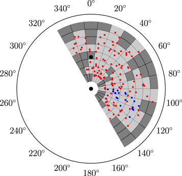
Figure 1. Galactocentric positions and Milky Way disk coverage of the VLA survey H ii regions. The Galactic Center is the black point at the origin and the Sun is the black point 8.34 kpc in the direction θ = 0°. The colored points are the H ii regions in the pilot survey (blue) and main survey (red). The Galactic disk is divided into 120 bins of size 12° in Galactocentric azimuth, over the azimuth range −30° to 150°, and 2 kpc in Galactocentric radius, up to 18 kpc. Bins that contain at least one nebulae are colored light gray, whereas empty bins are dark gray.
Download figure:
Standard image High-resolution imageOur final H ii region target catalog contains 147 unique nebulae. Table 1 lists information about these H ii regions: the WISE Catalog name; the VLA project in which it was observed (13A-030 is the pilot survey and 15B-178 is the main survey); the WISE infrared position; the WISE infrared radius, RIR; the estimated 9 GHz RRL flux density, S9 GHz,L; the telescope and reference for the previous RRL detection; the previously measured RRL-to-continuum brightness ratio, SL/SC, and derived electron temperature, Te; and the reference for the RRL-to-continuum brightness ratio and electron temperature.
Table 1. Survey Targets
| Field | Project | R.A. | Decl. | RIR | S9 GHz,L | Telescopea | RRL | SL/SC | Te | Te |
|---|---|---|---|---|---|---|---|---|---|---|
| J2000 | J2000 | (arcsec) | (mJy | Authorb | (K) | Authorc | ||||
| (hh:mm:ss) | (dd:mm:ss) | beam−1) | ||||||||
| G005.883−0.399 | 15B-178 | 18:00:31.5 | −24:04:18.9 | 22.35 | 844.15 ± 5.77 | 140 Foot | Q06a | ⋯ | ⋯ | ⋯ |
| G009.598+0.199 | 15B-178 | 18:06:11.1 | −20:32:36.5 | 34.09 | 226.92 ± 20.00 | 140 Foot | L89 | ⋯ | ⋯ | ⋯ |
| G010.596−0.381 | 15B-178 | 18:10:24.6 | −19:57:08.4 | 60.00 | 586.69 ± 4.23 | 140 Foot | Q06a | 0.0686 ± 0.0006 | 9810 ± 90 | Q06b;B15 |
| G012.804−0.207 | 15B-178 | 18:14:15.0 | −17:55:56.4 | 21.15 | 3034.62 ± 23.85 | 140 Foot | Q06a | 0.0808 ± 0.0007 | 7620 ± 100 | Q06b;B15 |
| G013.880+0.285 | 15B-178 | 18:14:35.7 | −16:45:09.7 | 144.31 | 587.42 ± 5.00 | 140 Foot | Q06a | 0.1210 ± 0.0012 | 6960 ± 80 | Q06b;B15 |
| G015.212+0.167 | 15B-178 | 18:17:40.0 | −15:38:13.8 | 176.72 | 10.95 ± 0.11 | GBT | A15b | ⋯ | ⋯ | ⋯ |
| G017.336−0.146 | 15B-178 | 18:22:57.2 | −13:54:41.0 | 102.77 | 6.70 ± 0.18 | GBT | A11 | ⋯ | ⋯ | ⋯ |
| G017.928−0.677 | 15B-178 | 18:26:01.7 | −13:38:14.6 | 164.84 | 13.00 ± 0.30 | GBT | A11 | ⋯ | ⋯ | ⋯ |
| G018.584+0.344 | 15B-178 | 18:23:34.9 | −12:34:48.7 | 42.50 | 14.00 ± 0.28 | GBT | A11 | ⋯ | ⋯ | ⋯ |
| G019.030+0.423 | 15B-178 | 18:24:09.0 | −12:08:53.0 | 77.79 | 4.05 ± 0.38 | GBT | A11 | ⋯ | ⋯ | ⋯ |
| G019.716−0.261 | 15B-178 | 18:27:56.0 | −11:51:39.4 | 58.90 | 14.80 ± 0.27 | GBT | A15b | ⋯ | ⋯ | ⋯ |
| G019.728−0.113 | 15B-178 | 18:27:25.2 | −11:46:55.1 | 42.50 | 7.70 ± 0.20 | GBT | A11 | ⋯ | ⋯ | ⋯ |
| G020.227+0.110 | 15B-178 | 18:27:33.8 | −11:14:11.4 | 71.07 | 5.25 ± 0.12 | GBT | A11 | ⋯ | ⋯ | ⋯ |
| G020.363−0.014 | 15B-178 | 18:28:16.1 | −11:10:25.6 | 42.50 | 10.90 ± 0.24 | GBT | A11 | ⋯ | ⋯ | ⋯ |
| G021.386−0.255 | 15B-178 | 18:31:04.0 | −10:22:43.4 | 57.60 | 15.65 ± 0.14 | GBT | A11 | ⋯ | ⋯ | ⋯ |
| G021.603−0.169 | 15B-178 | 18:31:10.0 | −10:08:48.4 | 31.87 | 4.10 ± 0.20 | GBT | A15b | ⋯ | ⋯ | ⋯ |
| G023.041−0.399 | 15B-178 | 18:34:41.3 | −8:58:37.1 | 151.85 | 65.35 ± 0.66 | GBT | A11 | ⋯ | ⋯ | ⋯ |
| G023.423−0.216 | 15B-178 | 18:34:44.5 | −8:33:10.9 | 96.79 | 816.54 ± 3.65 | 140 Foot | Q06a | 0.1162 ± 0.0008 | 6500 ± 55 | Q06b;B15 |
| G023.661−0.252 | 15B-178 | 18:35:18.9 | −8:21:34.2 | 56.59 | 24.30 ± 0.23 | GBT | A11 | ⋯ | ⋯ | ⋯ |
| G023.787+0.223 | 15B-178 | 18:33:50.6 | −8:01:42.3 | 189.71 | 146.15 ± 22.69 | 140 Foot | L89 | ⋯ | ⋯ | ⋯ |
| G024.185+0.211 | 15B-178 | 18:34:37.6 | −7:40:51.3 | 178.07 | 176.92 ± 16.15 | 140 Foot | L89 | ⋯ | ⋯ | ⋯ |
| G024.724−0.084 | 15B-178 | 18:36:41.1 | −7:20:16.7 | 254.14 | 253.85 ± 26.92 | 140 Foot | L89 | ⋯ | ⋯ | ⋯ |
| G024.728+0.159 | 15B-178 | 18:35:49.5 | −7:13:20.1 | 75.57 | 42.20 ± 0.25 | GBT | A11 | ⋯ | ⋯ | ⋯ |
| G024.734+0.087 | 15B-178 | 18:36:05.6 | −7:15:01.3 | 85.58 | 93.95 ± 0.50 | GBT | A11 | ⋯ | ⋯ | ⋯ |
| G025.397+0.033 | 15B-178 | 18:37:30.8 | −6:41:08.8 | 39.69 | 88.46 ± 10.38 | 140 Foot | L89 | ⋯ | ⋯ | ⋯ |
| G025.398+0.562 | 15B-178 | 18:35:37.4 | −6:26:34.0 | 42.50 | 23.25 ± 0.15 | GBT | A11 | ⋯ | ⋯ | ⋯ |
| G025.477+0.040 | 15B-178 | 18:37:38.2 | −6:36:45.1 | 42.50 | 4.60 ± 0.20 | GBT | A11 | ⋯ | ⋯ | ⋯ |
| G026.597−0.024 | 15B-178 | 18:39:55.9 | −5:38:45.0 | 26.61 | 16.65 ± 0.25 | GBT | A15a | ⋯ | ⋯ | ⋯ |
| G027.210+0.282 | 15B-178 | 18:39:58.0 | −4:57:39.4 | 42.50 | 6.00 ± 0.17 | GBT | A15b | ⋯ | ⋯ | ⋯ |
| G027.562+0.084 | 13A-030 | 18:41:19.3 | −4:44:21.4 | 42.50 | 22.60 ± 0.15 | GBT | A11 | 0.1601 ± 0.0021 | 5827 ± 94 | B11;B15 |
| G028.320+1.243 | 15B-178 | 18:38:34.9 | −3:32:04.8 | 60.00 | 2.25 ± 0.10 | GBT | A15b | ⋯ | ⋯ | ⋯ |
| G028.451+0.001 | 15B-178 | 18:43:14.9 | −3:59:11.0 | 28.70 | 9.20 ± 0.20 | GBT | A15b | ⋯ | ⋯ | ⋯ |
| G028.581+0.145 | 15B-178 | 18:42:58.4 | −3:48:18.8 | 42.50 | 6.75 ± 0.10 | GBT | A11 | ⋯ | ⋯ | ⋯ |
| G029.019+0.165 | 15B-178 | 18:43:42.1 | −3:24:19.3 | 106.80 | 14.35 ± 0.19 | GBT | A11 | ⋯ | ⋯ | ⋯ |
| G029.770+0.219 | 15B-178 | 18:44:53.2 | −2:42:49.6 | 42.50 | 7.60 ± 0.10 | GBT | A11 | ⋯ | ⋯ | ⋯ |
| G029.816+2.225 | 15B-178 | 18:37:49.6 | −1:45:17.9 | 168.83 | 9.25 ± 0.16 | GBT | A15b | ⋯ | ⋯ | ⋯ |
| G029.956−0.020 | 15B-178 | 18:46:04.5 | −2:39:25.2 | 94.36 | 896.81 ± 3.69 | 140 Foot | Q06a | 0.0992 ± 0.0064 | 6510 ± 90 | Q06b;B15 |
| G030.211+0.428 | 15B-178 | 18:44:56.7 | −2:13:30.7 | 37.11 | 2.75 ± 0.20 | GBT | A15b | ⋯ | ⋯ | ⋯ |
| G031.269+0.064 | 15B-178 | 18:48:10.6 | −1:27:00.7 | 24.84 | 92.31 ± 10.38 | 140 Foot | L89 | ⋯ | ⋯ | ⋯ |
| G031.274+0.485 | 13A-030 | 18:46:41.9 | −1:15:43.8 | 83.38 | 4.15 ± 0.10 | GBT | A11 | 0.0944 ± 0.0042 | 8690 ± 462 | B11;B15 |
| G031.577+0.103 | 15B-178 | 18:48:35.9 | −1:09:28.0 | 117.27 | 80.77 ± 8.46 | 140 Foot | L89 | ⋯ | ⋯ | ⋯ |
| G032.030+0.048 | 15B-178 | 18:49:37.2 | +0:46:47.7 | 42.50 | 6.35 ± 0.13 | GBT | A11 | ⋯ | ⋯ | ⋯ |
| G032.272−0.226 | 13A-030 | 18:51:02.3 | +0:41:25.4 | 42.50 | 32.90 ± 0.14 | GBT | A11 | 0.0889 ± 0.0008 | 8238 ± 104 | B11;B15 |
| G032.272−0.226 | 15B-178 | 18:51:02.3 | +0:41:25.4 | 42.50 | 32.90 ± 0.14 | GBT | A11 | 0.0889 ± 0.0008 | 8238 ± 104 | B11;B15 |
| G032.733+0.209 | 13A-030 | 18:50:19.9 | +0:04:54.3 | 42.50 | 11.95 ± 0.27 | GBT | A11 | 0.1638 ± 0.0037 | 5856 ± 156 | B11;B15 |
| G032.876−0.423 | 13A-030 | 18:52:50.7 | +0:14:57.6 | 126.62 | 15.20 ± 0.32 | GBT | A11 | 0.1817 ± 0.0043 | 6074 ± 176 | B11;B15 |
| G032.928+0.607 | 13A-030 | 18:49:16.4 | +0:16:22.3 | 65.68 | 25.60 ± 0.09 | GBT | A11 | 0.0680 ± 0.0006 | 9843 ± 170 | B11;B15 |
| G032.976−0.334 | 13A-030 | 18:52:44.0 | +0:06:31.4 | 131.80 | 12.50 ± 0.20 | GBT | A11 | 0.1485 ± 0.0040 | 6411 ± 207 | B11;B15 |
| G033.643−0.229 | 15B-178 | 18:53:32.9 | +0:31:44.7 | 42.50 | 3.35 ± 0.16 | GBT | A11 | ⋯ | ⋯ | ⋯ |
| G034.041+0.053 | 13A-030 | 18:53:16.4 | +1:00:40.2 | 42.50 | 19.45 ± 0.20 | GBT | A11 | 0.1384 ± 0.0021 | 6105 ± 120 | B11;B15 |
| G034.133+0.471 | 13A- 030 | 18:51:57.1 | +1:17:01.3 | 42.50 | 58.55 ± 0.18 | GBT | A11 | 0.1021 ± 0.0005 | 7655 ± 63 | B11;B15 |
| G034.686+0.068 | 13A-030 | 18:54:23.8 | +1:35:31.5 | 42.50 | 21.75 ± 0.15 | GBT | A11 | 0.1492 ± 0.0026 | 5335 ± 112 | B11;B15 |
| G035.126−0.755 | 15B-178 | 18:58:07.6 | +1:36:30.0 | 169.39 | 36.85 ± 0.26 | GBT | A15b | ⋯ | ⋯ | ⋯ |
| G035.948−0.149 | 15B-178 | 18:57:28.4 | +2:37:01.0 | 42.50 | 3.35 ± 0.21 | GBT | A11 | ⋯ | ⋯ | ⋯ |
| G036.918+0.482 | 15B-178 | 18:56:59.9 | +3:46:04.5 | 29.02 | 6.25 ± 0.17 | GBT | A11 | ⋯ | ⋯ | ⋯ |
| G037.445−0.212 | 15B-178 | 19:00:26.2 | +3:55:11.2 | 124.08 | 17.35 ± 0.15 | GBT | A11 | ⋯ | ⋯ | ⋯ |
| G037.469−0.105 | 15B-178 | 19:00:05.9 | +3:59:22.0 | 41.03 | 5.14 ± 0.10 | Arecibo | B12 | ⋯ | ⋯ | ⋯ |
| G038.550+0.163 | 13A-030 | 19:01:07.7 | +5:04:22.6 | 42.50 | 15.50 ± 0.20 | GBT | A11 | 0.1008 ± 0.0016 | 8216 ± 167 | B11;B15 |
| G038.643−0.227 | 15B-178 | 19:02:41.5 | +4:58:37.5 | 42.50 | 5.30 ± 0.09 | GBT | A11 | ⋯ | ⋯ | ⋯ |
| G038.651+0.087 | 13A-030 | 19:01:35.3 | +5:07:43.9 | 42.50 | 8.70 ± 0.07 | GBT | A11 | 0.0738 ± 0.0015 | 9428 ± 245 | B11;B15 |
| G038.738−0.140 | 15B-178 | 19:02:33.4 | +5:06:05.0 | 105.52 | 9.75 ± 0.10 | GBT | A11 | ⋯ | ⋯ | ⋯ |
| G038.840+0.497 | 13A-030 | 19:00:28.5 | +5:28:58.5 | 84.39 | 7.45 ± 0.07 | GBT | A11 | 0.0734 ± 0.0020 | 9221 ± 317 | B11;B15 |
| G038.875+0.308 | 13A-030 | 19:01:12.5 | +5:25:41.8 | 42.50 | 27.05 ± 0.12 | GBT | A11 | 0.0822 ± 0.0008 | 8384 ± 116 | B11;B15 |
| G039.183−1.422 | 15B-178 | 19:07:56.9 | +4:54:31.2 | 60.00 | 4.95 ± 0.16 | GBT | A15b | ⋯ | ⋯ | ⋯ |
| G039.196+0.224 | 15B-178 | 19:02:05.8 | +5:40:32.2 | 60.00 | 2.32 ± 0.10 | Arecibo | B12 | ⋯ | ⋯ | ⋯ |
| G039.869+0.645 | 13A-030 | 19:01:49.3 | +6:27:45.5 | 68.19 | 10.80 ± 0.09 | GBT | A11 | 0.0708 ± 0.0013 | 9373 ± 214 | B11;B15 |
| G041.750+0.034 | 15B-178 | 19:07:29.9 | +7:51:27.3 | 121.00 | 2.90 ± 0.10 | GBT | A15b | ⋯ | ⋯ | ⋯ |
| G041.762+1.479 | 15B-178 | 19:02:19.9 | +8:31:54.0 | 268.99 | 2.35 ± 0.09 | GBT | A15b | ⋯ | ⋯ | ⋯ |
| G043.149+0.028 | 15B-178 | 19:10:07.7 | +9:05:47.0 | 35.18 | 3129.19 ± 10.23 | 140 Foot | Q06a | ⋯ | ⋯ | ⋯ |
| G043.240+0.131 | 15B-178 | 19:09:55.7 | +9:13:28.1 | 42.50 | 5.40 ± 0.17 | GBT | A11 | ⋯ | ⋯ | ⋯ |
| G043.432+0.521 | 13A-030 | 19:08:54.1 | +9:34:22.2 | 74.33 | 11.25 ± 0.15 | GBT | A11 | 0.1021 ± 0.0019 | 8338 ± 198 | B11;B15 |
| G043.523−0.648 | 15B-178 | 19:13:15.5 | +9:06:54.0 | 88.57 | 2.20 ± 0.18 | GBT | A11 | ⋯ | ⋯ | ⋯ |
| G043.818+0.393 | 13A-030 | 19:10:03.7 | +9:51:31.6 | 108.26 | 14.80 ± 0.09 | GBT | A11 | 0.0781 ± 0.0013 | 8802 ± 196 | B11;B15 |
| G043.818+0.395 | 15B-178 | 19:10:03.7 | +9:51:31.6 | 108.26 | 14.80 ± 0.09 | GBT | A11 | 0.0781 ± 0.0013 | 8802 ± 196 | B11;B15 |
| G043.968+0.993 | 15B-178 | 19:08:11.3 | +10:16:04.7 | 50.84 | 5.55 ± 0.25 | GBT | A15b | ⋯ | ⋯ | ⋯ |
| G044.417+0.536 | 13A-030 | 19:10:41.0 | +10:27:22.6 | 84.69 | 6.55 ± 0.08 | GBT | A11 | 0.0926 ± 0.0026 | 8492 ± 299 | B11;B15 |
| G044.501+0.335 | 13A-030 | 19:11:34.3 | +10:26:07.5 | 50.65 | 24.25 ± 0.12 | GBT | A11 | 0.1017 ± 0.0017 | 8350 ± 153 | B11;B15 |
| G045.197+0.738 | 13A-030 | 19:11:24.5 | +11:14:28.3 | 80.49 | 9.35 ± 0.10 | GBT | A11 | 0.0556 ± 0.0010 | 10841 ± 245 | B11;B15 |
| G045.391−0.725 | 15B-178 | 19:17:03.7 | +10:43:57.9 | 191.48 | 26.50 ± 0.26 | GBT | A11 | ⋯ | ⋯ | ⋯ |
| G046.173+0.533 | 15B-178 | 19:14:00.4 | +12:00:39.7 | 60.00 | 2.04 ± 0.04 | Arecibo | B12 | ⋯ | ⋯ | ⋯ |
| G048.719+1.147 | 15B-178 | 19:16:38.2 | +14:32:58.9 | 82.92 | 6.30 ± 0.32 | GBT | A15b | ⋯ | ⋯ | ⋯ |
| G049.399−0.490 | 15B-178 | 19:23:55.6 | +14:22:54.6 | 51.68 | 68.15 ± 0.23 | GBT | A11 | ⋯ | ⋯ | ⋯ |
| G049.690−0.166 | 15B-178 | 19:23:19.0 | +14:47:29.5 | 178.62 | 76.92 ± 7.69 | 140 Foot | L96 | ⋯ | ⋯ | ⋯ |
| G050.032+0.605 | 15B-178 | 19:21:09.8 | +15:27:24.2 | 139.55 | 5.50 ± 0.20 | GBT | A15b | ⋯ | ⋯ | ⋯ |
| G052.001+1.602 | 15B-178 | 19:21:21.4 | +17:39:45.1 | 49.60 | 2.00 ± 0.07 | GBT | A15b | ⋯ | ⋯ | ⋯ |
| G052.098+1.042 | 15B-178 | 19:23:37.1 | +17:29:01.8 | 122.52 | 38.40 ± 0.17 | GBT | A11 | ⋯ | ⋯ | ⋯ |
| G052.160+0.708 | 15B-178 | 19:24:58.5 | +17:22:49.6 | 67.26 | 7.00 ± 0.20 | GBT | A11 | ⋯ | ⋯ | ⋯ |
| G052.256+0.702 | 15B-178 | 19:25:11.2 | +17:27:43.9 | 120.73 | 5.30 ± 0.08 | Arecibo | B12 | ⋯ | ⋯ | ⋯ |
| G054.093+1.748 | 15B-178 | 19:24:58.5 | +19:34:32.6 | 81.06 | 2.60 ± 0.10 | GBT | A15b | ⋯ | ⋯ | ⋯ |
| G054.490+0.930 | 15B-178 | 19:28:49.9 | +19:32:08.0 | 245.76 | 4.95 ± 0.09 | GBT | A11 | ⋯ | ⋯ | ⋯ |
| G054.490+1.579 | 15B-178 | 19:26:24.4 | +19:50:41.1 | 87.52 | 3.50 ± 0.10 | GBT | A15b | ⋯ | ⋯ | ⋯ |
| G055.114+2.422 | 15B-178 | 19:24:29.9 | +20:47:33.2 | 146.16 | 28.75 ± 0.17 | GBT | A15b | 0.0423 ± 0.0003 | 13126 ± 144 | B11;B15 |
| G059.796+0.241 | 15B-178 | 19:42:32.9 | +23:50:02.4 | 159.46 | 53.38 ± 0.41 | GBT | B11 | 0.0975 ± 0.0008 | 9068 ± 120 | B11;B15 |
| G060.592+1.572 | 15B-178 | 19:39:11.2 | +25:10:59.4 | 126.28 | 13.05 ± 0.13 | GBT | A15b | ⋯ | ⋯ | ⋯ |
| G061.431+2.081 | 15B-178 | 19:39:02.7 | +26:09:52.0 | 143.57 | 3.65 ± 0.17 | GBT | A15b | ⋯ | ⋯ | ⋯ |
| G061.720+0.863 | 15B-178 | 19:44:23.6 | +25:48:44.2 | 72.00 | 9.30 ± 0.10 | GBT | A11 | ⋯ | ⋯ | ⋯ |
| G062.577+2.389 | 15B-178 | 19:40:21.9 | +27:18:45.9 | 141.52 | 31.60 ± 0.18 | GBT | A15b | ⋯ | ⋯ | ⋯ |
| G068.144+0.915 | 15B-178 | 19:59:09.7 | +31:21:32.3 | 160.08 | 23.91 ± 0.27 | GBT | B11 | 0.0697 ± 0.0009 | 10834 ± 207 | B11;B15 |
| G070.280+1.583 | 15B-178 | 20:01:47.8 | +33:31:33.4 | 53.06 | 328.08 ± 1.75 | GBT | B11 | ⋯ | ⋯ | ⋯ |
| G070.673+1.190 | 15B-178 | 20:04:24.0 | +33:38:59.2 | 120.63 | 2.65 ± 0.13 | GBT | A15b | ⋯ | ⋯ | ⋯ |
| G070.765+1.820 | 15B-178 | 20:02:03.9 | +34:03:47.8 | 86.97 | 12.10 ± 0.14 | GBT | A15b | ⋯ | ⋯ | ⋯ |
| G071.150+0.397 | 15B-178 | 20:08:50.5 | +33:37:30.8 | 144.06 | 33.75 ± 0.10 | GBT | A15b | ⋯ | ⋯ | ⋯ |
| G073.878+1.023 | 15B-178 | 20:13:34.7 | +36:15:00.4 | 71.21 | 7.80 ± 0.10 | GBT | A15b | ⋯ | ⋯ | ⋯ |
| G074.155+1.646 | 15B-178 | 20:11:45.0 | +36:49:26.5 | 95.39 | 3.70 ± 0.11 | GBT | A15b | ⋯ | ⋯ | ⋯ |
| G074.753+0.912 | 15B-178 | 20:16:27.5 | +36:54:57.7 | 91.43 | 6.40 ± 0.12 | GBT | A15b | ⋯ | ⋯ | ⋯ |
| G075.175−0.593 | 15B-178 | 20:23:50.1 | +36:24:39.5 | 306.78 | 8.80 ± 0.14 | GBT | A15b | ⋯ | ⋯ | ⋯ |
| G075.768+0.344 | 15B-178 | 20:21:41.2 | +37:26:02.9 | 197.80 | 273.60 ± 0.56 | GBT | B11 | 0.0790 ± 0.0004 | 8590 ± 47 | B11;B15 |
| G078.174−0.550 | 15B-178 | 20:32:30.2 | +38:52:15.1 | 160.63 | 10.20 ± 0.15 | GBT | A15b | ⋯ | ⋯ | ⋯ |
| G078.886+0.709 | 15B-178 | 20:29:24.7 | +40:11:18.7 | 174.84 | 9.75 ± 0.23 | GBT | A15b | ⋯ | ⋯ | ⋯ |
| G080.191+0.534 | 15B-178 | 20:34:13.7 | +41:08:14.5 | 53.88 | 4.85 ± 0.12 | GBT | A15b | ⋯ | ⋯ | ⋯ |
| G091.113+1.580 | 15B-178 | 21:09:36.0 | +50:13:22.5 | 278.16 | 37.75 ± 0.17 | GBT | A15b | ⋯ | ⋯ | ⋯ |
| G093.518+2.611 | 15B-178 | 21:15:22.5 | +52:40:39.6 | 107.51 | 4.45 ± 0.16 | GBT | A15b | ⋯ | ⋯ | ⋯ |
| G094.263−0.414 | 15B-178 | 21:32:32.7 | +51:02:19.3 | 100.14 | 2.10 ± 0.10 | GBT | A15b | ⋯ | ⋯ | ⋯ |
| G096.289+2.593 | 15B-178 | 21:28:42.4 | +54:37:05.8 | 193.20 | 23.60 ± 0.11 | GBT | A15b | 0.0570 ± 0.0009 | 11039 ± 314 | B11;B15 |
| G096.434+1.324 | 15B-178 | 21:35:20.3 | +53:47:14.1 | 91.59 | 5.05 ± 0.14 | GBT | A15b | ⋯ | ⋯ | ⋯ |
| G097.444+3.083 | 15B-178 | 21:32:14.7 | +55:45:52.4 | 95.94 | 2.00 ± 0.18 | GBT | A15b | ⋯ | ⋯ | ⋯ |
| G097.515+3.173 | 15B-178 | 21:32:10.8 | +55:52:44.6 | 122.86 | 33.60 ± 0.18 | GBT | A15b | ⋯ | ⋯ | ⋯ |
| G101.016+2.590 | 15B-178 | 21:54:19.5 | +57:43:06.4 | 101.64 | 3.40 ± 0.18 | GBT | A15b | ⋯ | ⋯ | ⋯ |
| G104.700+2.784 | 15B-178 | 22:16:25.9 | +60:03:01.8 | 102.78 | 6.25 ± 0.18 | GBT | A15b | ⋯ | ⋯ | ⋯ |
| G109.104−0.347 | 15B-178 | 22:59:09.0 | +59:28:36.7 | 95.34 | 6.00 ± 0.12 | GBT | A15b | ⋯ | ⋯ | ⋯ |
| G111.802+0.526 | 15B-178 | 23:16:32.4 | +61:19:49.6 | 96.95 | 5.10 ± 0.20 | GBT | A15b | ⋯ | ⋯ | ⋯ |
| G118.276+2.490 | 15B-178 | 00:07:14.9 | +64:57:44.9 | 239.84 | 2.35 ± 0.17 | GBT | A15b | ⋯ | ⋯ | ⋯ |
| G118.592+2.828 | 15B-178 | 00:09:40.8 | +65:20:50.2 | 161.64 | 3.30 ± 0.18 | GBT | A15b | ⋯ | ⋯ | ⋯ |
| G124.637+2.535 | 15B-178 | 01:07:47.3 | +65:21:12.5 | 165.16 | 18.30 ± 0.21 | GBT | A15b | 0.0576 ± 0.0012 | 10758 ± 288 | B11;B15 |
| G125.092+0.778 | 15B-178 | 01:10:51.9 | +63:34:06.7 | 136.99 | 2.85 ± 0.17 | GBT | A15b | ⋯ | ⋯ | ⋯ |
| G135.188+2.701 | 15B-178 | 02:42:24.6 | +62:54:07.3 | 142.05 | 6.05 ± 0.12 | GBT | A15b | ⋯ | ⋯ | ⋯ |
| G136.119+2.118 | 15B-178 | 02:47:33.7 | +61:58:48.1 | 127.23 | 3.30 ± 0.13 | GBT | A15b | ⋯ | ⋯ | ⋯ |
| G136.884+0.911 | 15B-178 | 02:48:55.9 | +60:33:38.8 | 805.95 | 69.23 ± 8.08 | 140 Foot | L89 | 0.0995 ± 0.0025 | 8204 ± 257 | B11;B15 |
| G141.084−1.063 | 15B-178 | 03:10:16.0 | +56:50:04.3 | 249.15 | 7.80 ± 0.12 | GBT | A15b | ⋯ | ⋯ | ⋯ |
| G148.474+1.982 | 15B-178 | 04:05:41.7 | +54:54:55.2 | 104.17 | 2.55 ± 0.14 | GBT | A15b | ⋯ | ⋯ | ⋯ |
| G150.859−1.115 | 15B-178 | 04:03:50.6 | +51:00:57.9 | 123.28 | 2.85 ± 0.13 | GBT | A15b | ⋯ | ⋯ | ⋯ |
| G154.646+2.438 | 15B-178 | 04:36:48.8 | +50:52:42.5 | 370.38 | 25.02 ± 0.33 | GBT | B11 | 0.0673 ± 0.0009 | 9734 ± 175 | B11;B15 |
| G189.830+0.417 | 15B-178 | 06:08:58.1 | +20:38:29.2 | 199.15 | 82.62 ± 1.35 | 140 Foot | Q06a | ⋯ | ⋯ | ⋯ |
| G192.638−0.008 | 15B-178 | 06:13:07.5 | +17:58:33.5 | 174.27 | 52.91 ± 0.44 | GBT | B11 | 0.0971 ± 0.0010 | 8833 ± 107 | B11;B15 |
| G196.448−1.673 | 15B-178 | 06:14:37.3 | +13:50:02.6 | 302.50 | 30.80 ± 0.37 | GBT | B11 | 0.0773 ± 0.0010 | 9945 ± 164 | B11;B15 |
| G201.535+1.597 | 15B-178 | 06:36:11.8 | +10:51:56.8 | 790.64 | 12.79 ± 0.26 | GBT | B11 | 0.0713 ± 0.0015 | 10063 ± 283 | B11;B15 |
| G212.021−1.309 | 15B-178 | 06:45:07.1 | +0:12:49.8 | 1075.77 | 50.00 ± 5.38 | 140 Foot | L96 | ⋯ | ⋯ | ⋯ |
| G218.737+1.850 | 15B-178 | 07:08:39.2 | −4:18:55.1 | 215.23 | 35.22 ± 0.28 | GBT | B11 | 0.0509 ± 0.0005 | 14578 ± 195 | B11;B15 |
| G224.158+1.213 | 15B-178 | 07:16:29.0 | −9:24:51.3 | 558.98 | 8.35 ± 0.12 | GBT | A15b | ⋯ | ⋯ | ⋯ |
| G227.760−0.127 | 15B-178 | 07:18:30.6 | −13:13:29.4 | 324.34 | 7.54 ± 0.09 | GBT | B11 | 0.0485 ± 0.0007 | 12495 ± 249 | B11;B15 |
| G231.481−4.401 | 15B-178 | 07:09:54.3 | −18:29:53.7 | 511.74 | 21.11 ± 0.49 | GBT | B11 | 0.1011 ± 0.0024 | 9098 ± 286 | B11;B15 |
| G233.753−0.193 | 15B-178 | 07:30:04.6 | −18:32:03.8 | 311.06 | 27.16 ± 0.41 | GBT | B11 | 0.0822 ± 0.0015 | 9482 ± 209 | B11;B15 |
| G243.244+0.406 | 15B-178 | 07:52:42.5 | −26:29:00.1 | 941.61 | 49.06 ± 0.47 | GBT | B11 | 0.0764 ± 0.0012 | 10220 ± 110 | Q06b;B15 |
| G253.694−0.414 | 15B-178 | 08:15:34.9 | −35:45:30.3 | 1540.80 | 42.31 ± 4.23 | 140 Foot | L89 | ⋯ | ⋯ | ⋯ |
| G341.207−0.232 | 15B-178 | 16:52:20.7 | −44:28:06.8 | 58.11 | 90.60 ± 0.45 | GBT | A15b | ⋯ | ⋯ | ⋯ |
| G348.691−0.826 | 15B-178 | 17:19:06.6 | −38:51:37.7 | 1328.28 | 3132.27 ± 13.38 | 140 Foot | Q06a | ⋯ | ⋯ | ⋯ |
| G351.246+0.673 | 15B-178 | 17:20:17.7 | −35:54:29.2 | 131.55 | 2251.35 ± 7.73 | 140 Foot | Q06a | 0.0896 ± 0.0006 | 8560 ± 70 | Q06b;B15 |
| G351.311+0.663 | 15B-178 | 17:20:31.2 | −35:51:37.7 | 119.03 | 3356.38 ± 10.69 | 140 Foot | Q06a | ⋯ | ⋯ | ⋯ |
Notes.
aOriginal RRL detection telescope. bOriginal RRL detection reference. cRRL-to-continuum flux ratio measurement and electron temperature derivation referenceReferences. L89, Lockman (1989); L96, Lockman et al. (1996); Q06a, Quireza et al. (2006a); Q06b, Quireza et al. (2006b); A11, Anderson et al. (2011); B11, Balser et al. (2011); B12, Bania et al. (2012); A15a, Anderson et al. (2015a); A15b, Anderson et al. (2015b); B15, Balser et al. (2015).
3. Observations and Data Reduction
We used the VLA to simultaneously observe radio-continuum and RRL emission toward our sample of 147 Galactic H ii regions. The data were acquired in the most compact (D) antenna configuration as part of two projects: the pilot survey (13A-030; 5 hr) in Feb and Apr 2013, and the main survey (15B-178; 30 hr) in Oct and Nov 2015. A summary of the observations is in Table 2.
Table 2. Observation Summary
| 13A-030 | 15B-178 | |
|---|---|---|
| Dates | 2013 Feb and Apr | 2015 Oct and Nov |
| Observing Time (hr) | 5 | 30 |
| H ii Region Targets | 20 | 128 |
| Primary Calibrators | 3C286 | 3C286, 3C48 |
| Secondary Calibrators | J1733−1304, J1822−0938 | J0019+7327, J0102+5824 |
| J1824+1044, J1922+1530 | J0244+6228, J0349+4609 | |
| J0358+5606, J0625+1440 | ||
| J0653−0625, J0735−1735 | ||
| J0804−2749, J1604−4441 | ||
| J1744−3116, J1820−2528 | ||
| J1822v0938, J1824+1044 | ||
| J1922+1530, J1924+3329 | ||
| J1925+2106, J2007+4029 | ||
| J2025+3343, J2137+5101 | ||
| J2137+5101 | ||
| J2148+6107 |
Download table as: ASCIITypeset image
The VLA X-band receiver covers the frequency range ∼8–12 GHz. We used the Wideband Interferometric Digital ARchitecture (WIDAR) correlator in the 8-bit sampler mode to simultaneously measure ∼8–10 GHz radio-continuum emission and eight hydrogen RRL transitions in both linear polarizations. The continuum data were measured by 16 low spectral resolution spectral windows (hereafter, continuum windows) covering 7.8–8.9 GHz and 9–10 GHz continuously. The RRL spectra were measured by eight high-spectral resolution (31.25 kHz) spectral windows (hereafter, spectral line windows), each with 16 MHz of frequency coverage. There are only seven Hα RRL transitions in this frequency range (H87α to H93α), so we tuned one of the spectral line windows to H109β. The native velocity resolution ranges from 0.9 km s−1 at H87α to 1.2 km s−1 at H93α, with a velocity coverage ranging from 488 km s−1 to 600 km s−1 for these transitions, respectively. In one observing session of the pilot survey, the spectral line window for H88α was mistuned, so we exclude that spectral window from these analyses. Table 3 lists the following properties for each spectral window: the center frequency, νcenter; the bandwidth; the number of channels; the channel width, Δν; the targeted RRL transition; and the RRL rest frequency, νRRL.
Table 3. Correlator Setup
| Window | νcenter | Bandwidth | Channels | Δν | RRL | νRRL |
|---|---|---|---|---|---|---|
| (MHz) | (MHz) | (kHz) | (MHz) | |||
| 0 | 7949.3 | 128 | 128 | 1000 | ⋯ | ⋯ |
| 1 | 8049.1 | 128 | 128 | 1000 | ⋯ | ⋯ |
| 2 | 8049.1 | 16 | 512 | 31.25 | H93α | 8045.605 |
| 3 | 8205.3 | 128 | 128 | 1000 | ⋯ | ⋯ |
| 4 | 8333.3 | 128 | 128 | 1000 | ⋯ | ⋯ |
| 5 | 8313.0 | 16 | 512 | 31.25 | H92α | 8309.385 |
| 6 | 8461.3 | 128 | 128 | 1000 | ⋯ | ⋯ |
| 7 | 8589.3 | 128 | 128 | 1000 | ⋯ | ⋯ |
| 8 | 8588.5 | 16 | 512 | 31.25 | H91α | 8584.823 |
| 9 | 8717.3 | 128 | 128 | 1000 | ⋯ | ⋯ |
| 10 | 8845.3 | 128 | 128 | 1000 | ⋯ | ⋯ |
| 11 | 8876.4 | 16 | 512 | 31.25 | H90α | 8872.571 |
| 12 | 9082.3 | 128 | 128 | 1000 | ⋯ | ⋯ |
| 13 | 9210.3 | 128 | 128 | 1000 | ⋯ | ⋯ |
| 14 | 9177.3 | 16 | 512 | 1000 | H89α | 9173.323 |
| 15 | 9338.3 | 128 | 128 | 1000 | ⋯ | ⋯ |
| 16 | 9466.3 | 128 | 128 | 1000 | ⋯ | ⋯ |
| 17 | 9491.9 | 16 | 512 | 31.25 | H88α | 9487.824 |
| 18 | 9594.3 | 128 | 128 | 1000 | ⋯ | ⋯ |
| 19 | 9722.3 | 128 | 128 | 1000 | ⋯ | ⋯ |
| 20 | 9850.3 | 128 | 128 | 1000 | ⋯ | ⋯ |
| 21a | 9821.1 | 16 | 512 | 31.25 | H87α | 9816.867 |
| 22 | 9887.3 | 16 | 512 | 31.25 | H109β | 9883.083 |
| 23 | 9978.3 | 128 | 128 | 1000 | ⋯ | ⋯ |
Note.
aSpectral window 21 was mistuned for one observing session in 13A-030.Download table as: ASCIITypeset image
Our targets are clustered into 12 observing sessions based on position, with ∼10 H ii regions per group. Every observing session begins with a ∼15 minute integration on a primary calibrator, which is used for the absolute flux, delay, and bandpass calibration, followed by a ∼10 minute integration on a secondary calibrator located near the H ii region science targets, which is used for the complex gain calibration. These calibrators are listed in Table 2. We observe each science target for 10–15 minutes to reach the necessary spectral sensitivity, then we return to the secondary calibrator for ∼5 more minutes. During each observing session, we repeat this process for each science target.
We use the Wenger Interferometry Software Package (WISP) to calibrate, reduce, and analyze these data (Wenger 2018). WISP is a Python wrapper for the Common Astronomy Software Applications package (CASA; McMullin et al. 2007). Although WISP was developed to reduce Australia Telescope Compact Array data for the Southern H ii Region Discovery Survey (Wenger et al. 2019), its modular framework can be applied to any radio interferometric data set. We follow the Wenger et al. (2019) data reduction process, which we briefly describe here.
3.1. Calibration
The WISP calibration pipeline derives calibration solution tables using the calibrator source data, flags radio frequency interference (RFI) and other bad data, and applies the calibration solutions to the science target data. We inspect both the calibration solutions and calibrated data to assess the quality of the calibration solutions and to manually flag bad data that was missed by the WISP automatic flagging routines. The most common issues we flag are (1) antennas with poor calibration solutions, (2) broad-frequency RFI that contaminates an entire spectral window, and (3) shadowed antennas. In rare cases, RFI can compromise nearly one-half of all of our spectral windows.
3.2. Imaging
We use the WISP imaging pipeline to automatically generate and clean images from the calibrated visibility data. We begin by regridding all of the data to a common kinematic local standard of rest (LSR) velocity frame with a channel width ΔvLSR = 1.2 km s−1. Using the TCLEAN task in CASA, we generate several images and data cubes: (1) a multi-scale, multifrequency synthesis (MS-MFS) continuum image of the combined continuum spectral windows, (2) an MS-MFS image of each continuum and spectral line window, and (3) a multi-scale data cube of each spectral line window. Following the strategy of Wenger et al. (2019), we use CLEAN masks from each spectral line window MS-MFS image to CLEAN the data cube for that spectral window.
Many of our observed H ii regions are spatially resolved. We increase our surface brightness sensitivity to resolved emission by uv-tapering our visibilities when generating images. This process, however, reduces our point-source sensitivity and worsens our angular resolution. Therefore, we generate both non-tapered and uv-tapered images/data cubes for each field. The latter are tapered to a synthesized half-power beamwidth (HPBW) of 15'', which is about twice the native VLA resolution at X band.
4. Data Analysis
The data analysis process for this survey closely follows the Wenger et al. (2019) strategy. Because multiple nebulae may be observed in a single VLA pointing, we first identify unique WISE Catalog sources in each 8–10 GHz MS-MFS continuum image. Emission is associated with the WISE Catalog nebulae as long as the peak continuum brightness pixel is within a circle centered on the WISE Catalog position with a radius equal to the WISE Catalog infrared radius. We manually locate these peak continuum brightness pixels for each nebula with detected radio-continuum emission.
Unlike Wenger et al. (2019), we wish to derive the total fluxes of extended sources in addition to their peak fluxes. We use a watershed segmentation algorithm to identify the pixels associated with the manually identified continuum peaks in our images and data cubes. This algorithm considers an image as a three-dimensional topological surface, where the image brightness corresponds to the "depth" of the surface. The algorithm identifies the basins that would be filled by flooding the surface from a given starting point (see Bertrand 2005). In cases where multiple starting points will flood the same basin (i.e., in confused fields), the algorithm divides the basin into separate regions for each flooding source. Hereafter, we will use "watershed region" to describe the regions identified by the watershed segmentation algorithm.
We set the manually identified continuum brightness peak locations as the flooding sources for the watershed segmentation algorithm. Using the MS-MFS images clipped at five times the spatial rms noise, we run the algorithm to identify the watershed regions associated with each continuum source. Figure 2 shows an example region identified by this algorithm. We use the clipped continuum images to avoid low-brightness noise spikes in the watershed regions, but, as a result, we also miss faint emission associated with the nebulae. Therefore, our total continuum fluxes are systematically underestimated, especially for faint sources.

Figure 2. Watershed regions in a ∼2 GHz combined MS-MFS continuum image. This field is centered on G019.728−0.113 and contains three WISE Catalog H ii regions. The black contours are at 5, 10, 20, and 50 times the spatial rms noise (∼0.6 mJy beam−1 at the field center), and the yellow dashed circles represent the position and infrared radii of the WISE Catalog nebulae. The manually identified peak continuum brightness pixels are indicated by the colored plus symbols, and the watershed regions by the colored contours. These regions were created using the MS-MFS image clipped at five times the spatial rms noise to avoid including noise spikes in the watershed regions. These nebulae are examples of continuum quality factors (QF) A, B, and C, as indicated in the legend (see Section 5.1).
Download figure:
Standard image High-resolution imageFor each continuum source we measure the brightness and total flux at the location of the peak brightness and within the watershed region, respectively. The uncertainty of the peak continuum brightness is derived as the spatial rms of the CLEAN residual image divided by the VLA primary beam response at the peak continuum brightness position. To compute the uncertainty on the total continuum flux, we must consider that the spatial noise in an interferometric image is correlated on the scale of the synthesized beam. The variance in the sum of the brightnesses of N pixels within a region is
where σi is the spatial rms of the CLEAN residual image divided by the VLA primary beam response at the position of the ith pixel, ρij is the correlation coefficient between the ith and jth pixels, and the sums are taken over all N pixels within the region. We use the two-dimensional Gaussian synthesized beam to define the correlation coefficient:

where
Δx and Δy are the angular separations between the ith and jth pixels in the east–west and north–south directions, respectively, and θmaj, θmin, and ϕ are the synthesized beam major axis, minor axis, and north-through-east position angle, respectively. In the simple case where σi ≃ σj ≃ σ (i.e., the noise is constant across the source), Equation (1) reduces to

where Nbeam is the number of synthesized beams contained within the region. Many of our sources are extended or located near the edge of the primary beam, such that the primary beam response and noise varies across the source. Therefore, we use Equation (1) to derive the total continuum flux uncertainties.
We maximize our sensitivity to the faint RRL emission by averaging each observed Hnα RRL transition and both polarizations. This average spectrum is denoted by  . For non-tapered images, we extract spectra from each line spectral window data cube at the location of the peak continuum brightness. The
  spectrum is computed as the weighted average of the individual RRL transitions. The weights are given by
  where SC,i is the continuum brightness and rmsi is the spectral rms noise of the ith spectral window, both measured in the line-free region of the spectrum. For uv-tapered images, we spatially smooth the data cubes to a common beam size, then extract the spectra and compute the
  spectrum in the same fashion.
The total RRL emission within the watershed regions is extracted from the data cubes differently than for the peak position. For each pixel in the region, we measure the median continuum brightness in the line-free region of the spectrum, SC,i. Then we sum each pixel's spectrum, SL,i, weighted by the median continuum brightness in that pixel. The final extracted spectrum for this spectral window is normalized by the ratio of the median non-weighted sum and median weighted sum:
This complicated procedure correctly weights the final spectrum by the continuum level in each pixels' spectra, thereby maximizing the signal-to-noise ratio of the RRL and ensuring that the final spectrum has the correct flux density. The watershed region  spectrum is then computed using the same weighted average of the individual RRL transitions as for the peak positions.
Finally, we measure the  RRL properties. We first identify the line-free regions of the spectrum to estimate the spectral rms noise and to fit and remove a third-order polynomial baseline. Then we fit a Gaussian to the baseline-subtracted spectrum and measure the RRL brightness, the FWHM line width, and the LSR velocity.
5. Results
5.1. VLA Data Products
Our goal is to derive an accurate nebular electron temperature for as many of the observed Galactic H ii regions as possible. Given that some of these nebulae will be extremely faint, spatially resolved, and/or in confusing fields, no single data analysis method will work for each nebula. For each source, we therefore employ a suite of different analysis methods and then we pick the combination of non-tapered or uv-tapered images and peak position  or watershed region
  spectra that maximizes our RRL sensitivity and minimizes our electron temperature uncertainty.
We detect radio-continuum emission in 88 (59%) of the 148 observed fields. This low detection rate is a result of the relatively poor surface brightness sensitivity of the VLA. Many of the fields, however, contain multiple WISE Catalog H ii regions and/or H ii region candidates. We detect radio-continuum emission toward 114 known or candidate H ii regions. Table 4 lists the measured radio-continuum properties of these nebulae: the WISE Catalog source name; the MS-MFS synthesized frequency of the combined continuum spectral windows, νC; the peak continuum flux density,  a quality factor (QF) for the peak flux density,
  a column indicating whether the peak flux density was measured using the non-tapered (N) or uv-tapered (Y) image; the total flux density within the watershed region,
  a QF for the total flux density,
  and a column indicating whether the peak flux density was measured using the non-tapered or uv-tapered image. The MS-MFS synthesized frequency varies slightly for each field due to differences in data flagging. We select either non-tapered or uv-tapered based on which gives the smallest fractional uncertainty in the final electron temperature derivation (if the source also has a RRL detection), or which has the smallest fractional uncertainty in the continuum flux density. For resolved nebulae, the uv-tapered images typically have a smaller fractional electron temperature or continuum flux density uncertainty.
Table 4. Continuum Data Products
| Name | νC |

|

|
TaperPa |

|

|
TaperPa |
|---|---|---|---|---|---|---|---|
| (MHz) | (mJy beam−1) | (mJy) | |||||
| G005.885−00.393 | 8962.2 | 4516.01 ± 13.31 | A | N | 5254.49 ± 35.45 | A | N |
| G010.596−00.381 | 8962.2 | 395.02 ± 6.66 | A | Y | 907.08 ± 18.66 | A | Y |
| G013.880+00.285 | 8962.2 | 1696.64 ± 3.26 | A | Y | 3368.06 ± 10.64 | B | N |
| G017.336−00.146 | 8962.1 | 10.91 ± 0.29 | B | Y | 51.38 ± 0.84 | B | N |
| G017.928−00.677 | 8962.1 | 14.48 ± 0.37 | B | Y | 57.76 ± 1.07 | B | N |
| G018.584+00.344 | 8962.1 | 22.53 ± 0.82 | A | Y | 46.79 ± 1.20 | A | N |
| G018.630+00.309 | 8962.1 | 13.01 ± 4.37 | C | Y | 0.04 ± 0.18 | C | N |
| G019.677−00.134 | 8962.1 | 163.19 ± 3.36 | C | Y | 469.63 ± 7.10 | C | N |
| G019.728−00.113 | 8962.1 | 24.23 ± 0.40 | A | N | 27.24 ± 0.68 | A | N |
| G019.754−00.129 | 8962.1 | 46.45 ± 0.59 | B | N | 45.73 ± 1.01 | B | N |
| G020.227+00.110 | 8962.1 | 8.61 ± 0.13 | B | Y | 41.72 ± 0.36 | B | N |
| G020.363−00.014 | 8962.1 | 50.30 ± 0.09 | A | N | 58.28 ± 0.23 | A | N |
| G020.387−00.018 | 8962.1 | 8.58 ± 0.16 | B | Y | 26.85 ± 0.46 | B | Y |
| G021.386−00.255 | 8962.1 | 122.94 ± 0.12 | A | N | 136.88 ± 0.45 | A | N |
| G021.596−00.161 | 8962.2 | 5.70 ± 0.16 | A | N | 6.77 ± 0.26 | A | N |
| G021.603−00.169 | 8962.2 | 19.32 ± 0.15 | A | N | 27.62 ± 0.34 | A | N |
| G023.661−00.252 | 8962.2 | 30.11 ± 0.46 | B | Y | 152.51 ± 1.16 | B | N |
| G024.153+00.163 | 8962.2 | 10.94 ± 1.62 | C | N | 4.60 ± 1.14 | C | N |
| G024.166+00.250 | 8962.2 | 16.56 ± 0.79 | B | N | 17.44 ± 1.11 | B | N |
| G024.195+00.242 | 8962.2 | 9.77 ± 0.57 | B | N | 47.78 ± 1.69 | B | N |
| G024.713−00.125 | 8962.2 | 32.51 ± 2.11 | C | N | 138.58 ± 5.73 | C | N |
| G025.397+00.033 | 8962.2 | 229.49 ± 0.56 | B | N | 494.08 ± 2.57 | B | N |
| G025.398+00.562 | 8962.1 | 203.74 ± 0.36 | A | Y | 221.10 ± 1.21 | A | N |
| G025.401+00.021 | 8962.2 | 54.54 ± 0.60 | B | N | 150.97 ± 1.87 | B | N |
| G027.562+00.084 | 8898.2 | 47.71 ± 0.23 | A | N | 111.74 ± 0.71 | A | N |
| G028.320+01.243 | 8962.1 | 21.17 ± 0.04 | A | N | 30.22 ± 0.11 | A | N |
| G028.438+00.014 | 8962.2 | 4.01 ± 0.35 | A | N | 11.73 ± 0.74 | A | N |
| G028.451+00.001 | 8962.2 | 36.09 ± 0.30 | A | N | 84.81 ± 1.30 | A | N |
| G028.581+00.145 | 8962.2 | 25.87 ± 0.18 | A | N | 39.68 ± 0.41 | A | N |
| G029.770+00.219 | 8962.2 | 35.40 ± 0.16 | A | N | 72.53 ± 0.45 | A | N |
| G029.956−00.020 | 8962.2 | 1770.38 ± 4.48 | A | N | 4299.65 ± 22.54 | A | N |
| G030.211+00.428 | 8962.2 | 15.61 ± 0.04 | A | N | 25.81 ± 0.12 | A | N |
| G031.269+00.064 | 8962.2 | 2.70 ± 0.34 | A | N | 1.00 ± 0.22 | A | N |
| G031.279+00.061 | 8962.2 | 125.29 ± 0.35 | A | N | 306.72 ± 1.15 | A | N |
| G031.580+00.074 | 8962.2 | 13.41 ± 0.21 | B | N | 15.17 ± 0.38 | B | N |
| G032.030+00.048 | 8962.2 | 17.10 ± 0.19 | A | N | 25.83 ± 0.40 | A | N |
| G032.057+00.077 | 8962.2 | 13.36 ± 1.03 | C | Y | 94.17 ± 2.13 | C | N |
| G032.272−00.226 | 8962.2 | 147.87 ± 0.18 | A | N | 330.84 ± 0.75 | A | N |
| G032.928+00.606 | 8898.2 | 173.86 ± 0.27 | A | N | 336.64 ± 1.38 | A | N |
| G033.643−00.229 | 8962.2 | 6.37 ± 0.09 | A | Y | 10.85 ± 0.15 | A | N |
| G034.041+00.052 | 8962.2 | 25.97 ± 0.48 | A | Y | 83.27 ± 1.08 | A | N |
| G034.089+00.438 | 8962.2 | 34.42 ± 2.87 | C | N | 83.68 ± 7.38 | C | Y |
| G034.133+00.471 | 8962.2 | 378.58 ± 1.10 | A | Y | 517.00 ± 2.35 | A | N |
| G034.686+00.068 | 8962.2 | 55.42 ± 0.60 | A | Y | 107.24 ± 0.95 | A | N |
| G035.126−00.755 | 8962.2 | 123.85 ± 0.43 | A | Y | 241.91 ± 0.71 | A | N |
| G035.948−00.149 | 8962.2 | 12.05 ± 0.03 | A | N | 26.66 ± 0.08 | A | N |
| G036.870+00.462 | 8962.2 | 3.03 ± 0.31 | C | N | 9.77 ± 0.67 | C | N |
| G036.877+00.498 | 8962.2 | 1.22 ± 0.17 | C | N | 1.90 ± 0.22 | C | N |
| G036.918+00.482 | 8962.2 | 6.21 ± 0.08 | A | N | 7.56 ± 0.15 | A | N |
| G038.550+00.163 | 8962.2 | 54.11 ± 0.25 | A | N | 122.86 ± 0.77 | A | N |
| G038.643−00.227 | 8962.3 | 18.70 ± 0.05 | A | N | 24.79 ± 0.18 | A | N |
| G038.652+00.087 | 8962.2 | 19.77 ± 0.24 | A | N | 49.91 ± 0.96 | A | N |
| G038.840+00.495 | 8962.2 | 4.49 ± 0.09 | B | N | 84.27 ± 0.66 | B | N |
| G038.875+00.308 | 8962.2 | 279.04 ± 0.43 | A | N | 320.84 ± 1.04 | A | N |
| G039.183−01.422 | 8962.3 | 20.75 ± 0.15 | A | Y | 57.82 ± 0.30 | A | N |
| G039.196+00.224 | 8962.3 | 62.54 ± 0.06 | A | N | 67.11 ± 0.19 | A | N |
| G039.213+00.202 | 8962.3 | 5.13 ± 0.09 | B | N | 5.85 ± 0.16 | B | N |
| G039.864+00.645 | 8962.3 | 67.52 ± 0.51 | A | Y | 103.48 ± 0.79 | A | N |
| G043.146+00.013 | 8962.3 | 1434.45 ± 126.49 | B | Y | 1427.47 ± 158.00 | B | Y |
| G043.165−00.031 | 8962.3 | 2330.17 ± 78.58 | C | N | 3341.55 ± 144.37 | C | N |
| G043.168+00.019 | 8962.3 | 332.86 ± 17.06 | B | N | 600.24 ± 31.78 | B | N |
| G043.170−00.004 | 8962.3 | 4331.44 ± 149.88 | B | Y | 11158.53 ± 398.42 | B | Y |
| G043.432+00.516 | 8962.3 | 11.08 ± 0.35 | B | Y | 82.31 ± 0.83 | B | N |
| G043.523−00.648 | 8962.3 | 5.84 ± 0.04 | A | Y | 13.22 ± 0.09 | A | N |
| G043.818+00.395 | 8962.3 | 21.54 ± 0.97 | B | Y | 94.69 ± 1.89 | B | N |
| G043.968+00.993 | 8962.2 | 47.26 ± 0.07 | A | N | 49.81 ± 0.20 | A | N |
| G043.999+00.978 | 8962.2 | 22.23 ± 0.22 | C | N | 25.05 ± 0.42 | C | N |
| G044.501+00.332 | 8962.3 | 21.92 ± 1.24 | B | Y | 135.68 ± 2.23 | B | N |
| G044.503+00.349 | 8962.3 | 7.16 ± 0.36 | A | N | 8.58 ± 0.54 | A | N |
| G045.197+00.740 | 8962.3 | 7.76 ± 0.18 | B | N | 140.36 ± 1.42 | B | N |
| G048.719+01.147 | 8962.4 | 37.12 ± 0.10 | A | Y | 69.80 ± 0.29 | A | N |
| G049.399−00.490 | 8962.4 | 166.98 ± 7.12 | A | Y | 232.47 ± 8.75 | A | N |
| G052.098+01.042 | 8962.3 | 287.77 ± 0.50 | A | Y | 432.07 ± 0.89 | A | N |
| G052.232+00.735 | 8962.4 | 68.65 ± 4.32 | C | Y | 162.56 ± 5.42 | C | N |
| G054.093+01.748 | 8962.3 | 18.84 ± 0.03 | A | Y | 34.60 ± 0.08 | A | Y |
| G054.490+01.579 | 8962.3 | 24.30 ± 0.06 | A | Y | 44.24 ± 0.13 | A | N |
| G054.543+01.560 | 8962.3 | 3.73 ± 0.26 | C | Y | 3.52 ± 0.21 | C | N |
| G055.114+02.422 | 8962.3 | 138.55 ± 1.25 | A | Y | 618.76 ± 2.79 | B | N |
| G060.592+01.572 | 8962.3 | 55.66 ± 0.22 | A | Y | 166.35 ± 0.51 | A | N |
| G061.720+00.863 | 8962.7 | 90.28 ± 0.16 | A | N | 97.51 ± 0.38 | A | N |
| G062.577+02.389 | 8962.7 | 51.31 ± 0.28 | B | N | 359.10 ± 1.71 | B | N |
| G068.144+00.915 | 8962.7 | 42.25 ± 1.61 | B | Y | 302.02 ± 4.24 | B | N |
| G070.280+01.583 | 8962.6 | 542.61 ± 15.70 | A | Y | 1930.78 ± 37.24 | A | N |
| G070.293+01.599 | 8962.6 | 3550.27 ± 9.03 | A | N | 5690.67 ± 39.20 | A | N |
| G070.304+01.595 | 8962.6 | 245.05 ± 9.37 | A | N | 1829.40 ± 41.28 | A | N |
| G070.329+01.589 | 8962.6 | 1067.39 ± 23.78 | B | N | 2670.68 ± 65.51 | B | N |
| G070.673+01.190 | 8962.6 | 260.40 ± 0.72 | A | Y | 407.26 ± 1.43 | A | N |
| G070.765+01.820 | 8962.6 | 28.79 ± 0.52 | A | Y | 173.85 ± 1.36 | B | N |
| G071.150+00.397 | 8962.7 | 208.43 ± 0.25 | A | N | 392.62 ± 0.92 | A | N |
| G073.878+01.023 | 8962.6 | 75.77 ± 0.09 | A | N | 120.61 ± 0.26 | A | N |
| G074.155+01.646 | 8962.6 | 10.25 ± 0.04 | A | N | 37.97 ± 0.21 | A | N |
| G074.753+00.912 | 8962.6 | 55.70 ± 0.07 | A | N | 74.69 ± 0.20 | A | N |
| G075.768+00.344 | 8962.6 | 1059.58 ± 10.20 | A | Y | 4104.53 ± 20.67 | B | N |
| G078.114−00.550 | 8962.6 | 14.17 ± 3.03 | C | Y | 0.04 ± 0.10 | C | N |
| G078.174−00.550 | 8962.6 | 4.21 ± 0.19 | B | N | 23.01 ± 0.72 | B | N |
| G078.886+00.709 | 8962.6 | 83.02 ± 0.08 | A | N | 110.14 ± 0.25 | A | N |
| G080.191+00.534 | 8962.6 | 5.14 ± 0.09 | A | N | 40.72 ± 0.45 | A | N |
| G094.263−00.414 | 8963.1 | 4.40 ± 0.04 | B | Y | 18.73 ± 0.14 | B | N |
| G096.289+02.593 | 8963.1 | 27.93 ± 0.32 | B | N | 442.24 ± 2.68 | B | N |
| G096.434+01.324 | 8963.1 | 23.34 ± 0.10 | A | N | 36.94 ± 0.25 | A | N |
| G097.515+03.173 | 8963.1 | 131.05 ± 0.65 | A | Y | 508.47 ± 1.73 | B | N |
| G097.528+03.184 | 8963.1 | 41.23 ± 0.29 | A | N | 49.32 ± 0.55 | A | N |
| G101.016+02.590 | 8963.0 | 17.71 ± 0.06 | A | Y | 21.24 ± 0.14 | A | N |
| G104.700+02.784 | 8963.0 | 9.00 ± 0.17 | A | Y | 39.99 ± 0.36 | A | N |
| G109.104−00.347 | 8963.0 | 7.10 ± 0.07 | A | N | 19.36 ± 0.20 | A | N |
| G124.637+02.535 | 8963.4 | 252.56 ± 0.20 | A | N | 293.16 ± 0.62 | A | N |
| G125.092+00.778 | 8963.5 | 6.70 ± 0.02 | A | Y | 20.65 ± 0.07 | B | N |
| G135.188+02.701 | 8963.4 | 19.82 ± 0.09 | A | Y | 65.47 ± 0.18 | B | N |
| G141.084−01.063 | 8963.8 | 12.17 ± 0.19 | A | Y | 62.35 ± 0.37 | B | N |
| G150.859−01.115 | 8963.8 | 11.73 ± 0.10 | A | Y | 18.02 ± 0.15 | A | N |
| G196.448−01.673 | 8964.0 | 10.93 ± 0.47 | B | N | 350.13 ± 4.13 | B | N |
| G218.737+01.850 | 8964.1 | 202.41 ± 0.69 | A | Y | 554.43 ± 1.73 | A | N |
| G351.246+00.673 | 8962.2 | 7191.06 ± 24.43 | A | Y | 11722.85 ± 66.92 | A | N |
| G351.311+00.663 | 8962.2 | 2809.89 ± 29.27 | A | Y | 5561.39 ± 64.30 | A | N |
Note.
a"N" if non-tapered image measurement; "Y" if uv-tapered image measurement.The QF is a qualitative assessment of the accuracy of the continuum flux measurement. QF A detections are isolated, unresolved, and near the center of the primary beam, QF B detections are slightly resolved, in crowded fields, and/or are located off center from the primary beam, QF C detections are well-resolved, in very crowded fields, and/or are located near the edge of the primary beam. Any continuum sources that are confused/blended are assigned QF D. These nebulae are excluded from the tables and all subsequent analysis since we are unable to measure their continuum fluxes accurately. The three nebulae in Figure 2 are examples of each continuum QF: G019.728−00.113 is a QF A detection, G019.754−00.129 is a QF B detection because it is off center, and G019.677−00.134 is a QF C detection because it is resolved and near the edge of the primary beam.
We detect  RRL emission toward 82 (72%) of our 114 continuum sources. All RRL detections are toward previously known H ii regions. Figure 3 shows representative
  RRL detections with different signal-to-noise ratios. Our typical spectral rms noise is ∼1 mJy beam−1, about three times greater than what we estimated using the VLA sensitivity calculator. This decease in sensitivity is likely due to RFI that compromised entire spectral line spectral windows. We may be able to further increase our spectral line sensitivity by self-calibration.
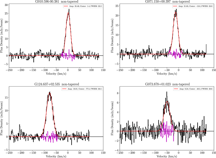
Figure 3. Representative  stacked spectra. The spectra for G010.596−00.381 (top left), G071.150+00.397 (top right), G124.637+02.535 (bottom left), and G073.878+01.023 (bottom right) span the range of typical RRL detection signal-to-noise ratios. The black histogram is the data, the red curve is the Gaussian fit with parameters listed in the legend, and the magenta curve is the fit residuals. These spectra were extracted from the non-tapered data cubes at the location of the peak continuum brightness.
Download figure:
Standard image High-resolution imageTable 5 lists the measured  RRL properties of our detections: the WISE Catalog source name; the weighted average frequency of the
  spectrum, νL, where the weights are the same as those used to average the individual RRL transitions (see Section 4); the amplitude of the Gaussian fit to the spectrum extracted from the location of peak continuum brightness,
  the spectral rms at this position, rmsP; the center LSR velocity of the fitted Gaussian,
  the FWHM line width of the fitted Gaussian, ΔVP; a column indicating whether the spectrum was extracted from the non-tapered (N) or uv-tapered (Y) image; the amplitude of the Gaussian fit to the spectrum summed within the watershed region,
  the spectral rms in this region, rmsT; the center LSR velocity of the fitted Gaussian,
  the FWHM line width of the fitted Gaussian, ΔVT; and a column indicating whether the spectrum was extracted from the non-tapered or uv-tapered image. As before, we use either the non-tapered or uv-tapered image, depending on which gives the smallest fractional uncertainty in the derived electron temperature. Unlike B15, we do not assign QFs to our RRL detections. Our spectral baselines are always flat and well modeled by a third-order polynomial, therefore, no qualitative assessment is necessary. Two nebulae, G005.885−00.393 and G070.293+01.599, are excluded from Table 5 because they have blended, non-Gaussian line profiles.
Table 5. RRL Data Products
| Name | νL |

|
rmsP |

|
ΔVP | TaperPa |

|
rmsT |

|
ΔVT | TaperTa |
|---|---|---|---|---|---|---|---|---|---|---|---|
| (MHz) | (mJy | (mJy | (km s−1) | (km s−1) | (mJy) | (mJy) | (km s−1) | (km s−1) | |||
| beam−1) | beam−1) | ||||||||||
| G009.612+00.205 | 8862.2 | 5.53 ± 0.39 | 1.19 | 2.5 ± 0.8 | 22.2 ± 1.9 | N | 2.71 ± 0.08 | 0.24 | 3.2 ± 0.3 | 22.1 ± 0.8 | N |
| G009.613+00.200 | 8786.3 | 81.07 ± 0.67 | 1.97 | 4.0 ± 0.1 | 20.4 ± 0.2 | Y | 133.99 ± 1.12 | 3.29 | 3.8 ± 0.1 | 20.5 ± 0.2 | N |
| G010.596−00.381 | 8816.4 | 59.07 ± 0.60 | 1.87 | 1.1 ± 0.1 | 23.3 ± 0.3 | Y | 107.40 ± 0.98 | 3.06 | 1.1 ± 0.1 | 23.1 ± 0.2 | Y |
| G010.621−00.380 | 8789.6 | 80.22 ± 0.52 | 1.67 | −0.5 ± 0.1 | 24.8 ± 0.2 | N | 3.61 ± 0.03 | 0.10 | −0.7 ± 0.1 | 24.9 ± 0.2 | N |
| G010.623−00.385 | 8737.2 | 175.69 ± 1.08 | 4.12 | 1.1 ± 0.1 | 35.0 ± 0.2 | Y | 182.71 ± 0.99 | 4.03 | 0.9 ± 0.1 | 39.9 ± 0.2 | N |
| G012.805−00.196 | 8779.1 | 1097.15 ± 3.02 | 11.78 | 36.3 ± 0.0 | 36.4 ± 0.1 | Y | 2079.31 ± 5.80 | 22.02 | 36.7 ± 0.0 | 34.5 ± 0.1 | Y |
| G012.813−00.200 | 8767.2 | 199.79 ± 1.44 | 4.85 | 30.2 ± 0.1 | 27.2 ± 0.2 | N | 74.74 ± 0.65 | 2.20 | 30.4 ± 0.1 | 27.7 ± 0.3 | N |
| G013.880+00.285 | 8806.2 | 267.42 ± 0.64 | 1.90 | 52.4 ± 0.0 | 21.5 ± 0.1 | Y | 530.66 ± 1.35 | 4.06 | 52.0 ± 0.0 | 21.6 ± 0.1 | Y |
| G017.928−00.677 | 8738.1 | ⋯ | ⋯ | ⋯ | ⋯ | ⋯ | 10.52 ± 1.04 | 3.06 | 38.4 ± 1.0 | 21.1 ± 2.5 | Y |
| G018.584+00.344 | 8806.1 | 3.57 ± 0.35 | 1.09 | 14.4 ± 1.2 | 24.1 ± 3.0 | Y | 7.58 ± 0.60 | 1.80 | 14.3 ± 0.9 | 22.2 ± 2.1 | Y |
| G019.677−00.134 | 8595.3 | 18.57 ± 1.27 | 4.14 | 54.7 ± 0.9 | 27.0 ± 2.4 | Y | 50.04 ± 2.52 | 8.33 | 55.6 ± 0.7 | 26.6 ± 1.6 | N |
| G019.728−00.113 | 8883.1 | 4.09 ± 0.34 | 1.08 | 53.6 ± 1.0 | 25.3 ± 2.5 | Y | 3.29 ± 0.25 | 0.81 | 52.9 ± 0.9 | 25.0 ± 2.3 | N |
| G020.363−00.014 | 8832.6 | 7.16 ± 0.32 | 0.98 | 55.1 ± 0.5 | 22.3 ± 1.2 | N | 7.90 ± 0.34 | 1.05 | 55.5 ± 0.5 | 22.5 ± 1.1 | N |
| G021.603−00.169 | 8886.8 | 2.67 ± 0.30 | 0.87 | −4.9 ± 1.3 | 23.0 ± 3.8 | Y | ⋯ | ⋯ | ⋯ | ⋯ | ⋯ |
| G023.661−00.252 | 8885.9 | 5.28 ± 0.34 | 1.03 | 66.5 ± 0.7 | 22.2 ± 1.7 | Y | 26.59 ± 1.08 | 3.17 | 67.2 ± 0.4 | 20.5 ± 1.0 | Y |
| G024.195+00.242 | 8819.2 | 3.38 ± 0.50 | 1.53 | 33.0 ± 1.8 | 24.3 ± 4.8 | Y | 3.52 ± 0.55 | 1.72 | 31.9 ± 1.9 | 25.1 ± 5.0 | N |
| G025.397+00.033 | 8826.1 | 20.71 ± 0.28 | 0.94 | −14.0 ± 0.2 | 28.0 ± 0.4 | N | 35.95 ± 0.56 | 1.88 | −14.0 ± 0.2 | 27.3 ± 0.5 | N |
| G025.398+00.562 | 8775.9 | 15.47 ± 0.27 | 0.98 | 11.7 ± 0.3 | 32.0 ± 0.6 | Y | 15.69 ± 0.29 | 1.07 | 11.5 ± 0.3 | 31.3 ± 0.7 | N |
| G025.401+00.021 | 8867.2 | 10.30 ± 0.55 | 1.73 | −10.7 ± 0.6 | 24.3 ± 1.5 | Y | 12.38 ± 0.51 | 1.54 | −10.2 ± 0.4 | 22.4 ± 1.1 | N |
| G026.597−00.024 | 8892.9 | 7.09 ± 0.21 | 0.80 | 17.3 ± 0.5 | 34.6 ± 1.2 | N | 15.57 ± 0.51 | 1.78 | 18.6 ± 0.5 | 30.0 ± 1.1 | Y |
| G027.562+00.084 | 8542.6 | 15.65 ± 0.53 | 1.55 | 88.2 ± 0.3 | 20.4 ± 0.8 | Y | 18.08 ± 0.59 | 1.74 | 88.2 ± 0.3 | 20.8 ± 0.8 | N |
| G028.320+01.243 | 8893.2 | 1.77 ± 0.26 | 0.65 | −40.5 ± 1.1 | 15.0 ± 2.7 | N | 1.76 ± 0.30 | 0.86 | −39.6 ± 4.5 | 34.1 ± 21.9 | N |
| G028.451+00.001 | 8840.4 | 5.07 ± 0.32 | 1.10 | −7.2 ± 0.9 | 28.7 ± 2.2 | Y | 5.96 ± 0.36 | 1.20 | −6.9 ± 0.8 | 27.2 ± 1.9 | N |
| G028.581+00.145 | 8860.3 | 2.84 ± 0.24 | 0.76 | −13.1 ± 1.0 | 24.4 ± 2.5 | N | 3.58 ± 0.28 | 0.94 | −13.0 ± 1.0 | 26.9 ± 2.6 | N |
| G029.770+00.219 | 8778.8 | 5.85 ± 0.38 | 1.15 | −30.9 ± 0.7 | 21.6 ± 1.7 | Y | 7.10 ± 0.47 | 1.39 | −30.9 ± 0.7 | 21.4 ± 1.6 | N |
| G030.211+00.428 | 8715.8 | 2.83 ± 0.37 | 0.97 | −10.8 ± 1.1 | 16.6 ± 2.6 | Y | 3.00 ± 0.38 | 1.02 | −11.5 ± 1.1 | 17.6 ± 2.6 | N |
| G031.580+00.074 | 8828.1 | 3.51 ± 0.46 | 1.04 | 100.4 ± 0.8 | 12.0 ± 1.8 | N | 3.27 ± 0.39 | 0.93 | 100.8 ± 0.8 | 13.5 ± 1.9 | N |
| G032.030+00.048 | 8848.2 | 5.13 ± 0.39 | 0.99 | 89.8 ± 0.6 | 15.3 ± 1.3 | Y | 4.81 ± 0.31 | 0.80 | 90.3 ± 0.5 | 16.1 ± 1.2 | N |
| G032.272−00.226 | 8819.0 | 21.61 ± 0.40 | 1.32 | 22.9 ± 0.2 | 26.5 ± 0.6 | Y | 27.01 ± 0.49 | 1.63 | 22.9 ± 0.2 | 26.9 ± 0.6 | N |
| G032.928+00.606 | 8590.7 | 13.70 ± 0.29 | 1.00 | −37.9 ± 0.3 | 28.9 ± 0.7 | N | 20.89 ± 0.49 | 1.63 | −38.2 ± 0.3 | 26.9 ± 0.7 | N |
| G034.041+00.052 | 8776.4 | 4.10 ± 0.40 | 1.26 | 36.9 ± 1.1 | 23.6 ± 2.7 | Y | 12.60 ± 0.91 | 2.80 | 37.7 ± 0.8 | 22.7 ± 1.9 | Y |
| G034.133+00.471 | 8801.3 | 42.46 ± 0.44 | 1.41 | 36.1 ± 0.1 | 24.6 ± 0.3 | Y | 56.32 ± 0.58 | 1.86 | 36.1 ± 0.1 | 24.6 ± 0.3 | N |
| G034.686+00.068 | 8724.2 | 7.06 ± 0.37 | 1.15 | 50.5 ± 0.6 | 23.8 ± 1.4 | Y | 14.29 ± 0.63 | 1.94 | 50.4 ± 0.5 | 22.4 ± 1.1 | Y |
| G035.126−00.755 | 8814.3 | 17.99 ± 0.40 | 1.17 | 35.0 ± 0.2 | 20.0 ± 0.5 | Y | 34.45 ± 0.71 | 2.05 | 35.3 ± 0.2 | 19.9 ± 0.5 | N |
| G035.948−00.149 | 8872.5 | 1.87 ± 0.24 | 0.74 | 51.4 ± 1.4 | 22.6 ± 3.6 | N | 3.15 ± 0.41 | 1.19 | 49.3 ± 1.4 | 21.0 ± 3.6 | N |
| G038.550+00.163 | 8758.9 | 11.79 ± 0.37 | 1.18 | 27.6 ± 0.4 | 23.7 ± 0.9 | Y | 14.88 ± 0.46 | 1.46 | 27.7 ± 0.4 | 23.8 ± 0.9 | N |
| G038.643−00.227 | 8762.5 | 2.70 ± 0.41 | 1.12 | 69.4 ± 1.4 | 18.5 ± 3.5 | Y | 3.81 ± 0.64 | 1.61 | 68.4 ± 1.3 | 15.6 ± 3.3 | Y |
| G038.840+00.495 | 8764.1 | ⋯ | ⋯ | ⋯ | ⋯ | ⋯ | 7.57 ± 0.98 | 2.80 | −42.8 ± 1.3 | 20.3 ± 3.2 | Y |
| G038.875+00.308 | 8808.9 | 25.36 ± 0.26 | 0.89 | −13.4 ± 0.1 | 27.8 ± 0.3 | N | 27.91 ± 0.31 | 1.07 | −13.8 ± 0.2 | 28.3 ± 0.4 | N |
| G039.196+00.224 | 8787.5 | 4.51 ± 0.24 | 0.84 | −21.7 ± 0.8 | 28.7 ± 1.9 | N | 4.88 ± 0.27 | 0.95 | −21.1 ± 0.8 | 29.2 ± 2.0 | N |
| G039.864+00.645 | 8738.8 | 5.21 ± 0.34 | 1.14 | −41.3 ± 0.9 | 27.3 ± 2.1 | Y | 8.57 ± 0.51 | 1.72 | −42.0 ± 0.8 | 27.6 ± 2.0 | N |
| G043.146+00.013 | 8708.1 | 134.45 ± 0.75 | 2.67 | 8.7 ± 0.1 | 30.2 ± 0.2 | Y | 101.01 ± 0.52 | 1.86 | 8.5 ± 0.1 | 31.1 ± 0.2 | Y |
| G043.151+00.011 | 8695.6 | 62.31 ± 0.51 | 1.84 | 5.8 ± 0.1 | 31.8 ± 0.3 | N | 48.52 ± 0.35 | 1.27 | 6.0 ± 0.1 | 31.9 ± 0.3 | N |
| G043.162+00.005 | 8768.7 | 42.28 ± 0.66 | 2.22 | 6.5 ± 0.2 | 27.0 ± 0.5 | N | 15.82 ± 0.21 | 0.70 | 6.2 ± 0.2 | 27.1 ± 0.4 | N |
| G043.165−00.031 | 8665.8 | 154.87 ± 2.24 | 8.99 | 6.8 ± 0.3 | 38.8 ± 0.7 | N | 128.59 ± 1.59 | 6.41 | 7.5 ± 0.2 | 39.0 ± 0.6 | N |
| G043.168+00.019 | 8762.5 | 46.09 ± 0.53 | 1.69 | 9.9 ± 0.1 | 24.1 ± 0.3 | N | 20.67 ± 0.22 | 0.70 | 9.8 ± 0.1 | 24.1 ± 0.3 | N |
| G043.170−00.004 | 8670.2 | 223.40 ± 0.87 | 3.38 | 7.8 ± 0.1 | 36.0 ± 0.2 | Y | 851.52 ± 2.80 | 10.04 | 4.5 ± 0.0 | 30.7 ± 0.1 | Y |
| G043.175+00.025 | 8739.0 | 40.65 ± 0.58 | 2.02 | 14.9 ± 0.2 | 28.7 ± 0.5 | N | 22.55 ± 0.27 | 0.95 | 14.9 ± 0.2 | 29.6 ± 0.4 | N |
| G043.432+00.516 | 8896.0 | ⋯ | ⋯ | ⋯ | ⋯ | ⋯ | 6.81 ± 0.97 | 2.92 | −11.8 ± 1.8 | 25.1 ± 5.6 | Y |
| G043.818+00.395 | 8881.8 | ⋯ | ⋯ | ⋯ | ⋯ | ⋯ | 8.70 ± 0.60 | 2.11 | −8.5 ± 1.0 | 31.0 ± 2.6 | Y |
| G043.968+00.993 | 8789.7 | 3.87 ± 0.24 | 0.87 | −25.5 ± 1.0 | 31.9 ± 2.5 | N | 3.92 ± 0.26 | 0.94 | −25.4 ± 1.0 | 31.2 ± 2.6 | N |
| G044.501+00.332 | 8806.0 | 2.80 ± 0.29 | 0.85 | −41.6 ± 1.1 | 22.0 ± 2.8 | Y | 6.46 ± 0.37 | 1.05 | −43.4 ± 0.5 | 19.7 ± 1.3 | Y |
| G048.719+01.147 | 8828.4 | 3.70 ± 0.32 | 1.05 | −25.6 ± 1.1 | 26.5 ± 2.8 | Y | 6.51 ± 0.55 | 1.79 | −25.9 ± 1.1 | 26.6 ± 2.8 | N |
| G049.399−00.490 | 8880.6 | 21.50 ± 0.43 | 1.34 | 62.7 ± 0.2 | 22.7 ± 0.5 | Y | 24.46 ± 0.40 | 1.28 | 61.5 ± 0.2 | 24.1 ± 0.5 | Y |
| G052.098+01.042 | 8835.7 | 24.43 ± 0.33 | 1.15 | 37.5 ± 0.2 | 29.3 ± 0.5 | Y | 36.72 ± 0.47 | 1.63 | 37.3 ± 0.2 | 28.7 ± 0.4 | N |
| G052.232+00.735 | 8756.0 | 5.54 ± 0.90 | 2.72 | −1.1 ± 2.2 | 26.2 ± 6.9 | Y | 19.84 ± 1.48 | 4.37 | −2.3 ± 0.8 | 20.8 ± 1.8 | Y |
| G055.114+02.422 | 8859.8 | 6.60 ± 0.30 | 1.08 | −73.6 ± 0.7 | 32.8 ± 1.8 | Y | 29.62 ± 0.78 | 2.87 | −74.8 ± 0.4 | 32.6 ± 1.0 | Y |
| G060.592+01.572 | 8864.6 | 3.93 ± 0.32 | 1.05 | −50.2 ± 1.1 | 27.2 ± 2.7 | Y | 11.25 ± 0.76 | 2.50 | −48.5 ± 0.9 | 26.8 ± 2.2 | Y |
| G061.720+00.863 | 8808.8 | 7.00 ± 0.67 | 2.11 | −69.6 ± 1.2 | 25.9 ± 3.3 | N | 7.39 ± 0.78 | 2.42 | −68.4 ± 1.3 | 24.5 ± 3.3 | N |
| G062.577+02.389 | 8747.3 | 8.53 ± 0.98 | 2.95 | −71.2 ± 1.3 | 22.3 ± 3.2 | Y | 24.80 ± 2.49 | 7.44 | −72.0 ± 1.1 | 22.0 ± 2.7 | Y |
| G070.280+01.583 | 8782.7 | 49.01 ± 0.86 | 2.68 | −23.6 ± 0.2 | 23.4 ± 0.5 | Y | 186.56 ± 1.83 | 5.95 | −25.1 ± 0.1 | 25.3 ± 0.3 | Y |
| G070.304+01.595 | 8763.0 | 72.95 ± 1.10 | 3.53 | −18.2 ± 0.2 | 24.5 ± 0.4 | Y | 51.50 ± 0.84 | 2.63 | −17.6 ± 0.2 | 23.4 ± 0.4 | N |
| G070.329+01.589 | 8694.4 | 157.24 ± 2.52 | 8.96 | −18.4 ± 0.2 | 30.4 ± 0.6 | Y | 123.82 ± 1.89 | 6.77 | −17.8 ± 0.2 | 30.6 ± 0.5 | N |
| G070.765+01.820 | 8843.3 | ⋯ | ⋯ | ⋯ | ⋯ | ⋯ | 13.56 ± 1.53 | 4.85 | −78.1 ± 1.4 | 24.9 ± 3.4 | N |
| G071.150+00.397 | 8783.3 | 34.14 ± 0.49 | 1.56 | −12.2 ± 0.2 | 24.2 ± 0.4 | Y | 38.36 ± 0.62 | 1.99 | −12.2 ± 0.2 | 24.6 ± 0.5 | Y |
| G073.878+01.023 | 8815.2 | 6.24 ± 0.32 | 1.12 | −49.5 ± 0.7 | 29.6 ± 1.8 | N | 8.50 ± 0.41 | 1.47 | −50.3 ± 0.7 | 30.8 ± 1.8 | N |
| G074.155+01.646 | 8798.0 | 4.15 ± 0.46 | 1.18 | −32.2 ± 0.9 | 15.9 ± 2.0 | Y | 5.86 ± 0.74 | 1.88 | −31.6 ± 1.0 | 15.7 ± 2.3 | Y |
| G074.753+00.912 | 8840.0 | 5.45 ± 0.33 | 1.04 | −48.9 ± 0.7 | 23.7 ± 1.7 | N | 6.42 ± 0.37 | 1.25 | −49.6 ± 0.8 | 27.9 ± 1.9 | N |
| G075.768+00.344 | 8789.4 | 100.01 ± 0.64 | 2.09 | −8.6 ± 0.1 | 25.5 ± 0.2 | Y | 364.25 ± 1.98 | 6.65 | −8.7 ± 0.1 | 27.0 ± 0.2 | Y |
| G078.886+00.709 | 8821.1 | 12.24 ± 0.37 | 1.04 | −1.9 ± 0.3 | 19.1 ± 0.7 | N | 15.90 ± 0.46 | 1.31 | −1.9 ± 0.3 | 19.5 ± 0.7 | N |
| G096.289+02.593 | 8873.2 | 4.36 ± 0.29 | 0.97 | −87.5 ± 0.9 | 26.8 ± 2.1 | Y | 27.37 ± 0.93 | 3.18 | −97.7 ± 0.5 | 28.3 ± 1.1 | Y |
| G096.434+01.324 | 8856.1 | 3.89 ± 0.28 | 0.85 | −77.8 ± 0.8 | 21.8 ± 1.9 | Y | 4.08 ± 0.29 | 0.88 | −77.9 ± 0.8 | 21.8 ± 1.8 | N |
| G097.515+03.173 | 8865.1 | 9.56 ± 0.29 | 1.00 | −76.8 ± 0.4 | 28.0 ± 1.0 | Y | 35.06 ± 0.79 | 2.72 | −74.4 ± 0.3 | 28.2 ± 0.7 | Y |
| G097.528+03.184 | 8901.3 | 4.34 ± 0.26 | 0.79 | −71.6 ± 0.7 | 23.1 ± 1.6 | N | 4.55 ± 0.25 | 0.79 | −72.0 ± 0.7 | 24.1 ± 1.6 | N |
| G101.016+02.590 | 8896.8 | 2.57 ± 0.36 | 0.92 | −70.2 ± 1.1 | 16.3 ± 2.7 | Y | 2.85 ± 0.38 | 1.00 | −70.2 ± 1.1 | 16.8 ± 2.7 | N |
| G109.104−00.347 | 8852.5 | 2.98 ± 0.29 | 0.90 | −44.1 ± 1.1 | 22.7 ± 2.6 | Y | 3.60 ± 0.34 | 1.09 | −44.4 ± 1.2 | 25.7 ± 2.9 | N |
| G124.637+02.535 | 8817.1 | 16.81 ± 0.27 | 0.96 | −77.5 ± 0.2 | 30.5 ± 0.6 | N | 18.35 ± 0.33 | 1.18 | −77.6 ± 0.3 | 30.7 ± 0.6 | N |
| G135.188+02.701 | 8974.4 | 2.61 ± 0.37 | 1.06 | −73.2 ± 1.4 | 19.9 ± 3.3 | Y | 6.42 ± 0.88 | 2.59 | −72.2 ± 2.8 | 31.9 ± 12.6 | Y |
| G141.084−01.063 | 8853.2 | ⋯ | ⋯ | ⋯ | ⋯ | ⋯ | 8.50 ± 1.15 | 3.15 | −25.2 ± 1.3 | 18.8 ± 3.2 | Y |
| G196.448−01.673 | 8872.6 | 4.71 ± 0.37 | 1.08 | 10.9 ± 0.8 | 20.8 ± 1.9 | Y | 27.00 ± 0.98 | 3.00 | 12.5 ± 0.4 | 22.6 ± 0.9 | Y |
| G351.246+00.673 | 8789.9 | 851.65 ± 2.69 | 8.64 | −0.4 ± 0.0 | 24.7 ± 0.1 | Y | 1474.38 ± 3.93 | 12.75 | −0.1 ± 0.0 | 25.1 ± 0.1 | Y |
| G351.311+00.663 | 8839.3 | 356.60 ± 1.81 | 5.76 | −6.9 ± 0.1 | 24.2 ± 0.1 | Y | 774.71 ± 2.46 | 7.79 | −6.2 ± 0.0 | 24.1 ± 0.1 | Y |
Note.
a"N" if non-tapered image measurement; "Y" if uv-tapered image measurement.5.2. Electron Temperatures
Thermal bremsstrahlung (free–free) emission is the primary source of H ii region radio-continuum emission. Its intensity depends on the plasma electron temperature, the plasma electron density, and the stellar ionizing photon rate. The free–free opacity of an H ii region in LTE is well-approximated by
where Te is the plasma electron temperature, EM is the emission measure, and ν is the frequency (Mezger & Henderson 1967). The emission measure is the integral of the squared electron number density, ne2, along the line-of-sight path through the nebula:  . An optically thin H ii region has a continuum brightness temperature TC ≃ τCTe. Without an independent determination of the emission measure, we are unable to use the continuum emission alone to derive the nebular electron temperature.
The RRL intensity and line width reveal the physical characteristics of an H ii region. The line center opacity of an H ii region in LTE is approximated by

where Δν is the full-width half-maximum (FWHM) line width in frequency units (Kardashev 1959; Mezger & Hoglund 1967). Similar to the continuum, we need an independent measurement of the emission measure in order to use the RRL properties to derive the electron temperature.
The typical hydrogen RRL line width for Galactic H ii regions is ∼25 km s−1 (Wenger et al. 2019). There are four physical effects that contribute to the RRL FWHM line width: (1) intrinsic broadening, due to the uncertainty principle; (2) collisional broadening, due to the collisions of the emitting atoms; (3) thermal Doppler broadening, due to the Maxwellian velocity distribution of emitting atoms in the plasma; and (4) nonthermal Doppler broadening. Of these, thermal and nonthermal Doppler broadening are the most significant contributors to the width of RRLs. The nonthermal (i.e., turbulent) components can only be constrained with additional information. RRL line width measurements for nebular plasma atoms other than hydrogen are needed, since atoms with different masses have different Maxwellian velocity distributions. Alternatively, the thermal contribution to the RRL line width can be determined by deriving the plasma temperature.
We derive the nebular electron temperature from the RRL-to-continuum brightness ratio. For an H ii region in LTE that is optically thin to both continuum and RRL emission, the ratio of the radio-continuum brightness temperature to the RRL peak brightness temperature is equal to the ratio of the continuum opacity to the line center opacity. This ratio is independent of the emission measure. A complete derivation of the electron temperature equation is in the Appendix. For RRLs near H90α, assuming the continuum and RRL emission originate in the same volume of gas, we find
where νL is the RRL frequency, SC is the continuum flux density, SL is the RRL center flux density, ΔV is the RRL FWHM line width in velocity units, and y+ is the ratio of the number density of singly ionized helium to hydrogen.
We use Equation (7) to derive the electron temperatures of the 72 nebulae in our sample with a VLA  RRL detection and a continuum QF A, B, or C. We only detect helium RRLs in a few, bright sources, so we assume y+ = 0.08 for all VLA detections, following Balser et al. (2011) and B15. Equation (7) is only weakly dependent on y+. A 10% increase from y+ = 0.08 results in a mere 0.6% increase in Te. We do not consider uncertainties in y+ in the subsequent analyses because the electron temperature uncertainties are typically much greater than 0.6%. Furthermore, we assume non-LTE effects and collisional broadening are negligible at these frequencies (see Balser et al. 1999). The RRL flux density, RRL FWHM line width, and continuum flux density are measured in the
  stacked spectrum, and the RRL frequency is the weighted average frequency of the individual RRL transitions. Again, the frequency weights are the same as those used to average the individual RRL transitions (see Section 4). In the Appendix, we show that this strategy can produce accurate electron temperatures.
Table 6 lists the WISE Catalog source name, the telescope used for the observation, the measured RRL-to-continuum flux ratios, the RRL FWHM line widths, and the derived electron temperatures for the B15 single dish and our VLA H ii region samples. This table only lists the highest quality electron temperature derivations; we remove all QF D sources from the B15 and VLA samples. The electron temperature uncertainties are computed by propagating the RRL-to-continuum flux ratio and FWHM line width uncertainties through Equation (7). For VLA sources, the "Type" column indicates whether the position of peak continuum brightness (P) or watershed region (T) is used to measure the RRL-to-continuum flux ratio. The "Taper" column identifies which data cube is used (N for non-tapered and Y for uv-tapered). We select the combination of "Type" and "Taper" that minimizes the fractional uncertainty in the derived electron temperature. In cases where the same source is detected in multiple surveys, we only list the VLA values, if available. If the source is not observed or detected in the VLA survey, we list the GBT values. If the source is not in the VLA survey nor the GBT survey, we list the 140 Foot values. Table 6 also includes information about the H ii region distances, which is discussed in Section 5.4.
Table 6. H ii Region Distances and Properties
| Name | Telescope | SL/SC | ΔV | Te | Typea | Taperb | d | R | Distancec | Distance |
|---|---|---|---|---|---|---|---|---|---|---|
| (km s−1) | (K) | (kpc) | (kpc) | Method | Reference | |||||
| G000.666−00.036 | 140 Foot | 0.0569 ± 0.0033 | 40.5 ± 0.4 | 8170 ± 180 | ⋯ | ⋯ |

|

|
P | R09c |
| G001.125−00.106 | 140 Foot | 0.1070 ± 0.0018 | 24.5 ± 0.2 | 7130 ± 70 | ⋯ | ⋯ | ⋯d | ⋯d | K | ⋯ |
| G003.266−00.061 | 140 Foot | 0.0978 ± 0.0100 | 25.3 ± 0.4 | 7440 ± 280 | ⋯ | ⋯ | ⋯d | ⋯d | K | ⋯ |
| G005.900−00.431 | 140 Foot | 0.0691 ± 0.0006 | 22.5 ± 0.2 | 11130 ± 170 | ⋯ | ⋯ |

|

|
P | S14 |
| G005.987−01.191 | 140 Foot | 0.0840 ± 0.0008 | 26.5 ± 0.2 | 8180 ± 70 | ⋯ | ⋯ | ⋯d | ⋯d | K | ⋯ |
| G008.137+00.232 | 140 Foot | 0.1019 ± 0.0007 | 25.4 ± 0.1 | 7090 ± 60 | ⋯ | ⋯ | ⋯d | ⋯d | K | ⋯ |
| G010.160−00.350 | 140 Foot | 0.0911 ± 0.0005 | 31.2 ± 0.2 | 6830 ± 30 | ⋯ | ⋯ | ⋯d | ⋯d | K | ⋯ |
| G010.308−00.150 | 140 Foot | 0.0874 ± 0.0005 | 31.6 ± 0.2 | 6800 ± 40 | ⋯ | ⋯ | ⋯d | ⋯d | K | ⋯ |
| G010.596−00.381 | VLA | 0.1506 ± 0.0015 | 23.1 ± 0.2 | 5704 ± 72 | T | Y |

|

|
P | Sa14 |
| G012.804−00.207 | 140 Foot | 0.0808 ± 0.0007 | 30.7 ± 0.3 | 7620 ± 100 | ⋯ | ⋯ |

|

|
P | I13 |
| G013.880+00.285 | VLA | 0.1568 ± 0.0004 | 21.5 ± 0.1 | 5848 ± 19 | P | Y |

|

|
P | S14 |
| G015.097−00.729 | 140 Foot | 0.0938 ± 0.0008 | 35.3 ± 0.3 | 5720 ± 60 | ⋯ | ⋯ |

|

|
P | X11 |
| G016.993+00.873 | 140 Foot | 0.0928 ± 0.0006 | 23.6 ± 0.1 | 6890 ± 60 | ⋯ | ⋯ |

|

|
K | ⋯ |
| G017.928−00.677 | VLA | 0.1461 ± 0.0158 | 21.1 ± 2.5 | 6269 ± 877 | T | Y |

|

|
K | ⋯ |
| G018.144−00.281 | 140 Foot | 0.1052 ± 0.0008 | 25.2 ± 0.2 | 7180 ± 70 | ⋯ | ⋯ |

|

|
K | ⋯ |
| G018.584+00.344 | VLA | 0.1547 ± 0.0135 | 22.2 ± 2.1 | 5712 ± 645 | T | Y |

|

|
K | ⋯ |
| G018.669+01.965 | 140 Foot | 0.0907 ± 0.0006 | 28.4 ± 0.2 | 7210 ± 60 | ⋯ | ⋯ |

|

|
K | ⋯ |
| G019.064−00.282 | 140 Foot | 0.2916 ± 0.0052 | 25.2 ± 0.3 | 5440 ± 70 | ⋯ | ⋯ |

|

|
K | ⋯ |
| G019.677−00.134 | VLA | 0.1166 ± 0.0063 | 26.6 ± 1.6 | 6141 ± 429 | T | N |

|

|
K | ⋯ |
| G019.728−00.113 | VLA | 0.1363 ± 0.0115 | 25.0 ± 2.3 | 5813 ± 629 | T | N |

|

|
K | ⋯ |
| G020.363−00.014 | VLA | 0.1416 ± 0.0067 | 22.5 ± 1.1 | 6150 ± 367 | T | N |

|

|
K | ⋯ |
| G020.728−00.105 | 140 Foot | 0.1249 ± 0.0035 | 26.5 ± 0.1 | 5590 ± 90 | ⋯ | ⋯ |

|

|
K | ⋯ |
| G021.603−00.169 | VLA | 0.1039 ± 0.0121 | 23.0 ± 3.8 | 7959 ± 1399 | P | Y |

|

|
K | ⋯ |
| G023.423−00.216 | 140 Foot | 0.1162 ± 0.0008 | 24.3 ± 0.1 | 6500 ± 55 | ⋯ | ⋯ |

|

|
P | B09 |
| G023.661−00.252 | VLA | 0.1737 ± 0.0079 | 20.5 ± 1.0 | 5583 ± 318 | T | Y |

|

|
K | ⋯ |
| G023.713+00.175 | 140 Foot | 0.1027 ± 0.0015 | 26.8 ± 0.4 | 6840 ± 110 | ⋯ | ⋯ |

|

|
K | ⋯ |
| G024.195+00.242 | VLA | 0.1190 ± 0.0187 | 24.3 ± 4.8 | 6692 ± 1465 | P | Y | ⋯d |

|
K | ⋯ |
| G024.456+00.489 | 140 Foot | 0.1020 ± 0.0008 | 29.2 ± 0.5 | 6370 ± 80 | ⋯ | ⋯ |

|

|
K | ⋯ |
| G024.844+00.093 | 140 Foot | 0.1326 ± 0.0012 | 24.9 ± 0.2 | 5860 ± 90 | ⋯ | ⋯ |

|

|
K | ⋯ |
| G025.382−00.151 | 140 Foot | 0.0974 ± 0.0027 | 25.6 ± 0.1 | 7460 ± 70 | ⋯ | ⋯ |

|

|
K | ⋯ |
| G025.397+00.033 | VLA | 0.0853 ± 0.0012 | 28.0 ± 0.4 | 7893 ± 142 | P | N |

|

|
K | ⋯ |
| G025.398+00.562 | VLA | 0.0774 ± 0.0014 | 32.0 ± 0.6 | 7610 ± 177 | P | Y |

|

|
K | ⋯ |
| G025.401+00.021 | VLA | 0.1074 ± 0.0046 | 22.4 ± 1.1 | 7871 ± 438 | T | N |

|

|
K | ⋯ |
| G025.867+00.118 | 140 Foot | 0.1189 ± 0.0016 | 27.3 ± 0.4 | 6120 ± 100 | ⋯ | ⋯ |

|

|
K | ⋯ |
| G027.562+00.084 | VLA | 0.1594 ± 0.0057 | 20.8 ± 0.8 | 5765 ± 261 | T | N |

|

|
K | ⋯ |
| G028.320+01.243 | VLA | 0.0819 ± 0.0125 | 15.0 ± 2.7 | 14189 ± 2932 | P | N |

|

|
K | ⋯ |
| G028.451+00.001 | VLA | 0.0923 ± 0.0058 | 27.2 ± 1.9 | 7576 ± 629 | T | N |

|

|
K | ⋯ |
| G028.581+00.145 | VLA | 0.0946 ± 0.0079 | 26.9 ± 2.6 | 7490 ± 837 | T | N |

|

|
K | ⋯ |
| G028.746+03.458 | GBT | 0.1106 ± 0.0007 | 21.0 ± 0.1 | 8399 ± 73 | ⋯ | ⋯ |

|

|
K | ⋯ |
| G029.770+00.219 | VLA | 0.1029 ± 0.0071 | 21.4 ± 1.6 | 8465 ± 755 | T | N |

|

|
K | ⋯ |
| G029.956−00.020 | 140 Foot | 0.0992 ± 0.0064 | 29.8 ± 0.1 | 6510 ± 90 | ⋯ | ⋯ |

|

|
P | Z14 |
| G030.211+00.428 | VLA | 0.1263 ± 0.0168 | 17.6 ± 2.6 | 8355 ± 1446 | T | N |

|

|
K | ⋯ |
| G030.758−00.047 | GBT | 0.0908 ± 0.0003 | 33.5 ± 0.1 | 6567 ± 30 | ⋯ | ⋯ |

|

|
K | ⋯ |
| G031.268+00.478 | GBT | 0.0944 ± 0.0042 | 23.2 ± 1.0 | 8690 ± 462 | ⋯ | ⋯ |

|

|
K | ⋯ |
| G031.580+00.074 | VLA | 0.2544 ± 0.0357 | 13.5 ± 1.9 | 5769 ± 992 | T | N |

|

|
P | Z14 |
| G032.030+00.048 | VLA | 0.2159 ± 0.0159 | 16.1 ± 1.2 | 5720 ± 519 | T | N |

|

|
P | S14 |
| G032.272−00.226 | VLA | 0.0850 ± 0.0016 | 26.9 ± 0.6 | 8207 ± 200 | T | N |

|

|
K | ⋯ |
| G032.733+00.209 | GBT | 0.1638 ± 0.0037 | 21.0 ± 0.4 | 5856 ± 156 | ⋯ | ⋯ |

|

|
K | ⋯ |
| G032.800+00.190 | GBT | 0.0750 ± 0.0004 | 29.5 ± 0.1 | 8625 ± 49 | ⋯ | ⋯ |

|

|
K | ⋯ |
| G032.870−00.427 | GBT | 0.1817 ± 0.0043 | 18.2 ± 0.4 | 6074 ± 176 | ⋯ | ⋯ |

|

|
K | ⋯ |
| G032.928+00.606 | VLA | 0.0723 ± 0.0016 | 28.9 ± 0.7 | 8641 ± 244 | P | N |

|

|
K | ⋯ |
| G032.982−00.338 | GBT | 0.1485 ± 0.0040 | 20.9 ± 0.5 | 6411 ± 207 | ⋯ | ⋯ |

|

|
K | ⋯ |
| G034.041+00.052 | VLA | 0.1489 ± 0.0119 | 22.7 ± 1.9 | 5809 ± 591 | T | Y |

|

|
K | ⋯ |
| G034.133+00.471 | VLA | 0.1140 ± 0.0013 | 24.6 ± 0.3 | 6858 ± 96 | T | N |

|

|
K | ⋯ |
| G034.256+00.136 | GBT | 0.0999 ± 0.0006 | 24.4 ± 0.1 | 8084 ± 55 | ⋯ | ⋯ |

|

|
K | ⋯ |
| G034.686+00.068 | VLA | 0.1232 ± 0.0058 | 22.4 ± 1.1 | 6876 ± 418 | T | Y |

|

|
K | ⋯ |
| G035.126−00.755 | VLA | 0.1428 ± 0.0032 | 19.9 ± 0.5 | 6793 ± 193 | T | N |

|

|
K | ⋯ |
| G035.197−01.756 | GBT | 0.0947 ± 0.0005 | 23.6 ± 0.0 | 8603 ± 40 | ⋯ | ⋯ |

|

|
P | Z09 |
| G035.948−00.149 | VLA | 0.1419 ± 0.0202 | 22.6 ± 3.6 | 6148 ± 1143 | P | N |

|

|
K | ⋯ |
| G037.754+00.560 | GBT | 0.1170 ± 0.0028 | 23.4 ± 0.8 | 7163 ± 246 | ⋯ | ⋯ |

|

|
K | ⋯ |
| G038.550+00.163 | VLA | 0.1149 ± 0.0038 | 23.8 ± 0.9 | 7019 ± 299 | T | N |

|

|
K | ⋯ |
| G038.643−00.227 | VLA | 0.1262 ± 0.0204 | 18.5 ± 3.5 | 7992 ± 1725 | P | Y |

|

|
K | ⋯ |
| G038.652+00.087 | GBT | 0.0738 ± 0.0015 | 27.0 ± 0.6 | 9428 ± 245 | ⋯ | ⋯ |

|

|
K | ⋯ |
| G038.840+00.495 | VLA | 0.0900 ± 0.0120 | 20.3 ± 3.2 | 9919 ± 1792 | T | Y |

|

|
K | ⋯ |
| G038.875+00.308 | VLA | 0.0882 ± 0.0009 | 27.8 ± 0.3 | 7719 ± 107 | P | N |

|

|
K | ⋯ |
| G039.196+00.224 | VLA | 0.0726 ± 0.0041 | 28.7 ± 1.9 | 8853 ± 658 | P | N |

|

|
K | ⋯ |
| G039.728−00.396 | GBT | 0.0874 ± 0.0020 | 25.7 ± 0.7 | 8503 ± 255 | ⋯ | ⋯ |

|

|
K | ⋯ |
| G039.864+00.645 | VLA | 0.0780 ± 0.0048 | 27.6 ± 2.0 | 8606 ± 707 | T | N |

|

|
K | ⋯ |
| G040.503+02.537 | GBT | 0.1074 ± 0.0006 | 22.4 ± 0.1 | 8223 ± 55 | ⋯ | ⋯ |

|

|
K | ⋯ |
| G043.146+00.013 | VLA | 0.0868 ± 0.0005 | 31.1 ± 0.2 | 6942 ± 48 | T | Y |

|

|
K | ⋯ |
| G043.165−00.031 | VLA | 0.0542 ± 0.0007 | 39.0 ± 0.6 | 8648 ± 144 | T | N |

|

|
P | Z13 |
| G043.168+00.019 | VLA | 0.1280 ± 0.0015 | 24.1 ± 0.3 | 6282 ± 92 | T | N |

|

|
P | Z13 |
| G043.170−00.004 | VLA | 0.0768 ± 0.0003 | 30.7 ± 0.1 | 7876 ± 35 | T | Y |

|

|
P | Z13 |
| G043.432+00.516 | VLA | 0.0930 ± 0.0138 | 25.1 ± 5.6 | 8119 ± 1883 | T | Y |

|

|
K | ⋯ |
| G043.818+00.395 | VLA | 0.0788 ± 0.0056 | 31.0 ± 2.6 | 7806 ± 750 | T | Y |

|

|
K | ⋯ |
| G043.968+00.993 | VLA | 0.0822 ± 0.0054 | 31.9 ± 2.5 | 7255 ± 647 | P | N |

|

|
K | ⋯ |
| G044.418+00.535 | GBT | 0.0926 ± 0.0026 | 24.3 ± 0.7 | 8492 ± 299 | ⋯ | ⋯ |

|

|
K | ⋯ |
| G044.501+00.332 | VLA | 0.1064 ± 0.0063 | 19.7 ± 1.3 | 9044 ± 694 | T | Y |

|

|
K | ⋯ |
| G045.197+00.740 | GBT | 0.0556 ± 0.0010 | 30.5 ± 0.6 | 10841 ± 245 | ⋯ | ⋯ |

|

|
K | ⋯ |
| G045.453+00.044 | GBT | 0.0871 ± 0.0007 | 27.6 ± 0.1 | 8026 ± 63 | ⋯ | ⋯ |

|

|
P | W14 |
| G046.495−00.241 | 140 Foot | 0.1989 ± 0.0071 | 20.1 ± 0.2 | 4860 ± 80 | ⋯ | ⋯ |

|

|
K | ⋯ |
| G048.719+01.147 | VLA | 0.0943 ± 0.0083 | 26.6 ± 2.8 | 7606 ± 900 | T | N |

|

|
K | ⋯ |
| G048.922−00.285 | 140 Foot | 0.0805 ± 0.0005 | 26.7 ± 0.2 | 8440 ± 60 | ⋯ | ⋯ |

|

|
P | W14 |
| G049.002−00.303 | 140 Foot | 0.1859 ± 0.0017 | 24.4 ± 0.2 | 8170 ± 50 | ⋯ | ⋯ |

|

|
P | W14 |
| G049.201−00.365 | 140 Foot | 0.0650 ± 0.0003 | 30.3 ± 0.1 | 9070 ± 70 | ⋯ | ⋯ |

|

|
P | W14 |
| G049.384−00.298 | 140 Foot | 0.0786 ± 0.0006 | 31.6 ± 0.3 | 8585 ± 65 | ⋯ | ⋯ |

|

|
K | ⋯ |
| G049.399−00.490 | VLA | 0.1167 ± 0.0021 | 24.1 ± 0.5 | 6675 ± 151 | T | Y |

|

|
P | W14 |
| G049.489−00.378 | GBT | 0.0903 ± 0.0003 | 30.2 ± 0.0 | 7166 ± 25 | ⋯ | ⋯ |

|

|
K | ⋯ |
| G052.098+01.042 | VLA | 0.0854 ± 0.0011 | 28.7 ± 0.4 | 7725 ± 134 | T | N |

|

|
P | O10 |
| G052.232+00.735 | VLA | 0.1083 ± 0.0085 | 20.8 ± 1.8 | 8258 ± 841 | T | Y |

|

|
K | ⋯ |
| G052.766+00.333 | GBT | 0.0841 ± 0.0011 | 25.4 ± 0.4 | 8970 ± 186 | ⋯ | ⋯ |

|

|
K | ⋯ |
| G055.114+02.422 | VLA | 0.0484 ± 0.0013 | 32.6 ± 1.0 | 11357 ± 409 | T | Y |

|

|
K | ⋯ |
| G059.796+00.241 | GBT | 0.0975 ± 0.0008 | 21.8 ± 0.2 | 9068 ± 120 | ⋯ | ⋯ |

|

|
K | ⋯ |
| G060.592+01.572 | VLA | 0.0692 ± 0.0048 | 26.8 ± 2.2 | 9883 ± 922 | T | Y |

|

|
K | ⋯ |
| G060.881−00.135 | GBT | 0.1229 ± 0.0010 | 21.2 ± 0.2 | 7463 ± 77 | ⋯ | ⋯ |

|

|
K | ⋯ |
| G061.473+00.094 | GBT | 0.0846 ± 0.0004 | 26.0 ± 0.1 | 8857 ± 43 | ⋯ | ⋯ |

|

|
K | ⋯ |
| G061.720+00.863 | VLA | 0.0777 ± 0.0076 | 25.9 ± 3.3 | 9170 ± 1282 | P | N |

|

|
K | ⋯ |
| G062.577+02.389 | VLA | 0.0766 ± 0.0079 | 22.0 ± 2.7 | 10626 ± 1470 | T | Y |

|

|
K | ⋯ |
| G063.164+00.449 | GBT | 0.0994 ± 0.0011 | 25.1 ± 0.1 | 7760 ± 90 | ⋯ | ⋯ |

|

|
K | ⋯ |
| G064.130−00.475 | GBT | 0.0973 ± 0.0005 | 23.9 ± 0.1 | 8452 ± 58 | ⋯ | ⋯ |

|

|
K | ⋯ |
| G068.144+00.915 | GBT | 0.0697 ± 0.0009 | 24.7 ± 0.3 | 10834 ± 207 | ⋯ | ⋯ |

|

|
K | ⋯ |
| G069.922+01.511 | GBT | 0.0712 ± 0.0003 | 27.0 ± 0.1 | 9703 ± 50 | ⋯ | ⋯ |

|

|
K | ⋯ |
| G070.280+01.583 | VLA | 0.0901 ± 0.0009 | 25.3 ± 0.3 | 8214 ± 109 | T | Y |

|

|
K | ⋯ |
| G070.293+01.599 | GBT | 0.0505 ± 0.0005 | 37.0 ± 0.2 | 10297 ± 121 | ⋯ | ⋯ |

|

|
K | ⋯ |
| G070.304+01.595 | VLA | 0.0992 ± 0.0017 | 23.4 ± 0.4 | 8211 ± 182 | T | N |

|

|
K | ⋯ |
| G070.329+01.589 | VLA | 0.0745 ± 0.0012 | 30.6 ± 0.5 | 8244 ± 170 | T | N |

|

|
K | ⋯ |
| G070.765+01.820 | VLA | 0.0896 ± 0.0105 | 24.9 ± 3.4 | 8412 ± 1317 | T | N |

|

|
K | ⋯ |
| G071.150+00.397 | VLA | 0.1035 ± 0.0016 | 24.2 ± 0.4 | 7551 ± 147 | P | Y |

|

|
K | ⋯ |
| G073.878+01.023 | VLA | 0.0744 ± 0.0037 | 30.8 ± 1.8 | 8177 ± 545 | T | N |

|

|
K | ⋯ |
| G074.155+01.646 | VLA | 0.1929 ± 0.0238 | 15.9 ± 2.0 | 6327 ± 980 | P | Y |

|

|
K | ⋯ |
| G074.753+00.912 | VLA | 0.0923 ± 0.0056 | 27.9 ± 1.9 | 7386 ± 592 | T | N |

|

|
K | ⋯ |
| G075.768+00.344 | VLA | 0.0900 ± 0.0005 | 27.0 ± 0.2 | 7743 ± 57 | T | Y |

|

|
P | A11 |
| G075.842+00.404 | GBT | 0.0751 ± 0.0003 | 30.5 ± 0.1 | 8363 ± 32 | ⋯ | ⋯ |

|

|
P | R12 |
| G076.155−00.286 | GBT | 0.0651 ± 0.0005 | 30.9 ± 0.2 | 9498 ± 119 | ⋯ | ⋯ |

|

|
K | ⋯ |
| G076.384−00.621 | GBT | 0.0407 ± 0.0002 | 42.0 ± 0.2 | 11245 ± 92 | ⋯ | ⋯ |

|

|
P | X13 |
| G078.032+00.606 | GBT | 0.0832 ± 0.0005 | 27.2 ± 0.2 | 8567 ± 86 | ⋯ | ⋯ |

|

|
P | R12 |
| G078.147+01.820 | GBT | 0.0910 ± 0.0008 | 24.6 ± 0.2 | 8596 ± 107 | ⋯ | ⋯ |

|

|
P | R12 |
| G078.886+00.709 | VLA | 0.1525 ± 0.0048 | 19.5 ± 0.7 | 6530 ± 260 | T | N |

|

|
P | R12 |
| G079.270+02.488 | GBT | 0.1161 ± 0.0021 | 20.8 ± 0.6 | 7977 ± 222 | ⋯ | ⋯ |

|

|
P | R12 |
| G079.293+01.296 | GBT | 0.0729 ± 0.0007 | 30.0 ± 0.1 | 8693 ± 86 | ⋯ | ⋯ |

|

|
K | ⋯ |
| G080.350+00.718 | GBT | 0.0699 ± 0.0007 | 26.5 ± 0.3 | 10250 ± 155 | ⋯ | ⋯ |

|

|
K | ⋯ |
| G080.362+01.212 | GBT | 0.1058 ± 0.0030 | 23.0 ± 0.7 | 7921 ± 294 | ⋯ | ⋯ |

|

|
P | R12 |
| G080.938−00.129 | GBT | 0.0774 ± 0.0004 | 28.7 ± 0.1 | 8853 ± 62 | ⋯ | ⋯ |

|

|
P | R12 |
| G081.681+00.540 | GBT | 0.0608 ± 0.0002 | 35.9 ± 0.1 | 8829 ± 36 | ⋯ | ⋯ |

|

|
P | R12 |
| G082.566+00.362 | GBT | 0.1038 ± 0.0011 | 23.4 ± 0.2 | 8030 ± 128 | ⋯ | ⋯ |

|

|
P | R12 |
| G083.792+03.269 | GBT | 0.0943 ± 0.0012 | 23.1 ± 0.3 | 8643 ± 184 | ⋯ | ⋯ |

|

|
P | R12 |
| G085.241+00.021 | GBT | 0.0799 ± 0.0011 | 26.9 ± 0.3 | 8824 ± 177 | ⋯ | ⋯ |

|

|
K | ⋯ |
| G092.920+02.823 | 140 Foot | 0.1308 ± 0.0028 | 24.8 ± 0.5 | 10840 ± 270 | ⋯ | ⋯ |

|

|
K | ⋯ |
| G096.289+02.593 | VLA | 0.0634 ± 0.0022 | 28.3 ± 1.1 | 10169 ± 464 | T | Y |

|

|
K | ⋯ |
| G096.434+01.324 | VLA | 0.1125 ± 0.0085 | 21.8 ± 1.8 | 7745 ± 762 | T | N |

|

|
K | ⋯ |
| G097.515+03.173 | VLA | 0.0711 ± 0.0017 | 28.2 ± 0.7 | 9226 ± 281 | T | Y |

|

|
P | H15 |
| G097.528+03.184 | VLA | 0.1029 ± 0.0060 | 24.1 ± 1.6 | 7726 ± 584 | T | N |

|

|
P | H15 |
| G101.016+02.590 | VLA | 0.1510 ± 0.0218 | 16.8 ± 2.7 | 7600 ± 1434 | T | N |

|

|
K | ⋯ |
| G108.191+00.586 | GBT | 0.0759 ± 0.0004 | 25.8 ± 0.1 | 9590 ± 59 | ⋯ | ⋯ |

|

|
P | C14 |
| G108.375−01.056 | GBT | 0.0806 ± 0.0009 | 26.1 ± 0.3 | 8992 ± 131 | ⋯ | ⋯ |

|

|
K | ⋯ |
| G108.764−00.952 | GBT | 0.0706 ± 0.0004 | 29.6 ± 0.2 | 9404 ± 81 | ⋯ | ⋯ |

|

|
K | ⋯ |
| G109.104−00.347 | VLA | 0.1998 ± 0.0222 | 25.7 ± 2.9 | 4061 ± 554 | T | N |

|

|
K | ⋯ |
| G110.099+00.042 | GBT | 0.0543 ± 0.0003 | 38.0 ± 0.2 | 9240 ± 75 | ⋯ | ⋯ |

|

|
K | ⋯ |
| G111.558+00.804 | GBT | 0.0829 ± 0.0005 | 27.1 ± 0.1 | 8483 ± 51 | ⋯ | ⋯ |

|

|
P | M09 |
| G111.612+00.371 | GBT | 0.0885 ± 0.0005 | 26.8 ± 0.1 | 8428 ± 68 | ⋯ | ⋯ |

|

|
K | ⋯ |
| G112.212+00.229 | GBT | 0.0777 ± 0.0008 | 28.8 ± 0.2 | 8641 ± 118 | ⋯ | ⋯ |

|

|
K | ⋯ |
| G115.785−01.561 | GBT | 0.0806 ± 0.0017 | 26.8 ± 0.6 | 8794 ± 242 | ⋯ | ⋯ |

|

|
K | ⋯ |
| G118.345+04.856 | 140 Foot | 0.0911 ± 0.0193 | 20.7 ± 0.3 | 9540 ± 1050 | ⋯ | ⋯ |

|

|
K | ⋯ |
| G124.637+02.535 | VLA | 0.0659 ± 0.0011 | 30.5 ± 0.6 | 9181 ± 198 | P | N |

|

|
K | ⋯ |
| G124.894+00.323 | GBT | 0.0781 ± 0.0031 | 27.0 ± 1.2 | 8975 ± 460 | ⋯ | ⋯ |

|

|
K | ⋯ |
| G128.772+02.009 | GBT | 0.0854 ± 0.0028 | 20.9 ± 0.7 | 10361 ± 427 | ⋯ | ⋯ |

|

|
K | ⋯ |
| G132.156−00.729 | GBT | 0.0769 ± 0.0006 | 24.9 ± 0.2 | 9785 ± 123 | ⋯ | ⋯ |

|

|
K | ⋯ |
| G133.712+01.221 | GBT | 0.0760 ± 0.0003 | 27.7 ± 0.0 | 8977 ± 38 | ⋯ | ⋯ |

|

|
P | X06;H06 |
| G133.781+01.428 | GBT | 0.0785 ± 0.0005 | 27.5 ± 0.1 | 8752 ± 74 | ⋯ | ⋯ |

|

|
P | X06;H06 |
| G135.188+02.701 | VLA | 0.1347 ± 0.0204 | 19.9 ± 3.3 | 7259 ± 1414 | P | Y |

|

|
K | ⋯ |
| G136.884+00.911 | GBT | 0.0995 ± 0.0025 | 23.5 ± 0.6 | 8204 ± 257 | ⋯ | ⋯ |

|

|
P | X06;H06 |
| G138.494+01.634 | GBT | 0.0969 ± 0.0014 | 23.8 ± 0.3 | 8302 ± 131 | ⋯ | ⋯ |

|

|
K | ⋯ |
| G141.084−01.063 | VLA | 0.1400 ± 0.0203 | 18.8 ± 3.2 | 7300 ± 1431 | T | Y |

|

|
K | ⋯ |
| G150.596−00.955 | GBT | 0.0671 ± 0.0005 | 27.8 ± 0.1 | 10016 ± 83 | ⋯ | ⋯ |

|

|
K | ⋯ |
| G151.609−00.233 | GBT | 0.0543 ± 0.0004 | 31.7 ± 0.2 | 10795 ± 98 | ⋯ | ⋯ |

|

|
K | ⋯ |
| G154.646+02.438 | GBT | 0.0673 ± 0.0009 | 28.6 ± 0.4 | 9734 ± 175 | ⋯ | ⋯ |

|

|
K | ⋯ |
| G155.372+02.613 | GBT | 0.0703 ± 0.0013 | 25.6 ± 0.5 | 10253 ± 309 | ⋯ | ⋯ |

|

|
K | ⋯ |
| G169.180−00.905 | GBT | 0.0872 ± 0.0013 | 23.1 ± 0.4 | 9345 ± 179 | ⋯ | ⋯ | ⋯d | ⋯d | K | ⋯ |
| G173.599+02.803 | GBT | 0.1060 ± 0.0013 | 20.9 ± 0.3 | 8612 ± 137 | ⋯ | ⋯ | ⋯d | ⋯d | K | ⋯ |
| G173.937+00.298 | GBT | 0.0935 ± 0.0014 | 23.0 ± 0.3 | 8829 ± 158 | ⋯ | ⋯ | ⋯d | ⋯d | K | ⋯ |
| G192.638−00.008 | GBT | 0.0971 ± 0.0010 | 22.1 ± 0.2 | 8833 ± 107 | ⋯ | ⋯ |

|

|
P | R10 |
| G196.448−01.673 | VLA | 0.0928 ± 0.0035 | 22.6 ± 0.9 | 8884 ± 435 | T | Y |

|

|
P | H07 |
| G209.037−19.377 | GBT | 0.0878 ± 0.0007 | 26.1 ± 0.0 | 8322 ± 55 | ⋯ | ⋯ |

|

|
P | S07;M07;K08 |
| G213.076−02.213 | GBT | 0.0564 ± 0.0006 | 28.6 ± 0.3 | 11343 ± 162 | ⋯ | ⋯ |

|

|
K | ⋯ |
| G213.703−12.601 | GBT | 0.0750 ± 0.0004 | 29.8 ± 0.1 | 8986 ± 65 | ⋯ | ⋯ |

|

|
K | ⋯ |
| G218.737+01.850 | GBT | 0.0702 ± 0.0007 | 24.6 ± 0.3 | 10671 ± 143 | ⋯ | ⋯ |

|

|
K | ⋯ |
| G220.524−02.759 | GBT | 0.0473 ± 0.0021 | 31.8 ± 1.7 | 12037 ± 725 | ⋯ | ⋯ |

|

|
K | ⋯ |
| G225.470−02.587 | GBT | 0.1141 ± 0.0020 | 22.6 ± 0.4 | 7537 ± 158 | ⋯ | ⋯ |

|

|
K | ⋯ |
| G227.760−00.127 | GBT | 0.0485 ± 0.0007 | 28.9 ± 0.4 | 12495 ± 249 | ⋯ | ⋯ |

|

|
K | ⋯ |
| G231.481−04.401 | GBT | 0.1011 ± 0.0024 | 20.5 ± 0.6 | 9098 ± 286 | ⋯ | ⋯ |

|

|
K | ⋯ |
| G233.753−00.193 | GBT | 0.0822 ± 0.0015 | 24.1 ± 0.4 | 9482 ± 209 | ⋯ | ⋯ |

|

|
K | ⋯ |
| G243.244+00.406 | GBT | 0.0793 ± 0.0014 | 22.3 ± 0.2 | 10477 ± 214 | ⋯ | ⋯ |

|

|
K | ⋯ |
| G345.284+01.463 | 140 Foot | 0.0891 ± 0.0006 | 24.1 ± 0.2 | 8530 ± 640 | ⋯ | ⋯ | ⋯d | ⋯d | K | ⋯ |
| G345.410−00.953 | 140 Foot | 0.1036 ± 0.0004 | 26.3 ± 0.1 | 6960 ± 50 | ⋯ | ⋯ | ⋯d | ⋯d | K | ⋯ |
| G348.249−00.971 | 140 Foot | 0.0918 ± 0.0005 | 28.2 ± 0.2 | 6610 ± 100 | ⋯ | ⋯ | ⋯d | ⋯d | K | ⋯ |
| G348.710−01.044 | 140 Foot | 0.1067 ± 0.0008 | 24.6 ± 0.2 | 7150 ± 90 | ⋯ | ⋯ |

|

|
P | W12 |
| G351.130+00.449 | 140 Foot | 0.1272 ± 0.0015 | 22.1 ± 0.2 | 6650 ± 70 | ⋯ | ⋯ | ⋯d | ⋯d | K | ⋯ |
| G351.170+00.704 | 140 Foot | 0.1283 ± 0.0009 | 25.9 ± 0.1 | 5610 ± 20 | ⋯ | ⋯ | ⋯d | ⋯d | K | ⋯ |
| G351.246+00.673 | VLA | 0.1131 ± 0.0003 | 25.1 ± 0.1 | 6772 ± 24 | T | Y |

|

|
P | W14 |
| G351.311+00.663 | VLA | 0.1301 ± 0.0004 | 24.1 ± 0.1 | 6230 ± 27 | T | Y |

|

|
P | W14 |
| G351.367+00.640 | 140 Foot | 0.1151 ± 0.0012 | 23.9 ± 0.1 | 6840 ± 40 | ⋯ | ⋯ |

|

|
P | W14 |
| G351.472−00.458 | 140 Foot | 0.1067 ± 0.0012 | 23.3 ± 0.5 | 7460 ± 120 | ⋯ | ⋯ | ⋯d | ⋯d | K | ⋯ |
| G351.646−01.252 | 140 Foot | 0.0848 ± 0.0005 | 28.1 ± 0.1 | 7620 ± 30 | ⋯ | ⋯ | ⋯d | ⋯d | K | ⋯ |
| G351.688−01.169 | 140 Foot | 0.1029 ± 0.0006 | 23.6 ± 0.1 | 7560 ± 90 | ⋯ | ⋯ | ⋯d | ⋯d | K | ⋯ |
| G352.597−00.188 | 140 Foot | 0.1172 ± 0.0025 | 20.9 ± 0.9 | 7560 ± 240 | ⋯ | ⋯ | ⋯d | ⋯d | K | ⋯ |
| G353.038+00.581 | 140 Foot | 0.1040 ± 0.0012 | 28.6 ± 0.1 | 6250 ± 30 | ⋯ | ⋯ | ⋯d | ⋯d | K | ⋯ |
| G353.092+00.857 | 140 Foot | 0.2296 ± 0.0024 | 28.7 ± 0.1 | 5630 ± 40 | ⋯ | ⋯ | ⋯d | ⋯d | K | ⋯ |
| G353.195+00.910 | 140 Foot | 0.0826 ± 0.0006 | 30.8 ± 0.2 | 7100 ± 40 | ⋯ | ⋯ | ⋯d | ⋯d | K | ⋯ |
| G353.408−00.381 | 140 Foot | 0.0912 ± 0.0008 | 24.0 ± 0.2 | 8480 ± 60 | ⋯ | ⋯ | ⋯d | ⋯d | K | ⋯ |
Notes.
a"P" if measured at the location of peak continuum brightness; "T" if measured within the watershed segmentation region b"N" if non-tapered image measurement; "Y" if uv-tapered image measurement c"K" for Monte Carlo kinematic distance; "P" for parallax distance dKinematic distances are unreliable in the direction of the Galactic center and anti-centerReferences. A11, Ando et al. (2011); B09, Brunthaler et al. (2009); C14, Choi et al. (2014); H06, Hachisuka et al. (2006); H07, Honma et al. (2007); H15, Hachisuka et al. (2015); I13, Immer et al. (2013); K08, Kim et al. (2008); M07, Menten et al. (2007); M09, Moscadelli et al. (2009); O10, Oh et al. (2010); RD09, Roman-Duval et al. (2009); R09a, Reid et al. (2009a); R09c, Reid et al. (2009b); R10, Rygl et al. (2010); R12, Rygl et al. (2012); S07, Sandstrom et al. (2007); S10, Sato et al. (2010); S14, Sato et al. (2014); Sa14, Sanna et al. (2014); U12, Urquhart et al. (2012); W12, Wu et al. (2012); W14, Wu et al. (2014); X06, Xu et al. (2006); X11, Xu et al. (2011); X13, Xu et al. (2013); Z09, Zhang et al. (2009); Z13, Zhang et al. (2013); Z14, Zhang et al. (2014).
In total, there are now 189 Galactic H ii regions with accurate electron temperature determinations. This is an increase of 99 nebulae (110%) over the B15 sample. A fraction of these nebulae have inaccurate distances, however, and cannot be used to investigate Galactic metallicity structure.
5.3. Comparison with Single Dish
Our sample combines measurements from three telescopes: the 140 Foot, the GBT, and the VLA. Each of these telescopes may be affected by systematics that lead to discrepancies between the derived electron temperatures because each is sampling a different volume of gas within and surrounding the H ii regions. For example, diffuse foreground and background emission may affect the single-dish observations, but such extended emission is filtered out by the VLA. In principle, there may be differences between the different single-dish measurements as well. Balser et al. (2011) find no significant difference between the derived electron temperatures for 16 nebulae observed by both the 140 Foot and the GBT. Here we compare the single-dish and VLA observations of 22 nebulae in common between the B15 single-dish catalog and our VLA catalog.
We first compare the fitted LSR velocity of these nebulae. The top panel of Figure 4 shows the difference between the single-dish RRL LSR velocity and that measured by the VLA for the 22 nebulae observed by the VLA and either the GBT or the 140 Foot. Here and in all subsequent analyses, we use the "best" combination of non-tapered or uv-tapered data cubes and continuum peak brightness location or watershed region for spectral extraction. "Best" means the combination of tapering and spectral extraction technique that minimizes the fractional uncertainty in the derived electron temperature. The single-dish and VLA LSR velocities are in good agreement, with a weighted mean difference of −0.09 ± 0.34 km s−1 (the error here is the uncertainty of the mean), a median difference of −1.28 km s−1, and a standard deviation of 1.59 km s−1. Throughout these analyses, we use the reciprocal variances of the fitted Gaussian parameters as the weights in the averages.
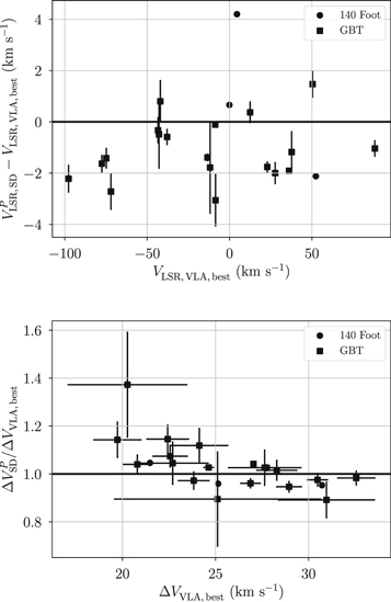
Figure 4. Difference between single-dish and VLA RRL LSR velocities (top) and ratio of single-dish to VLA RRL FWHM line widths (bottom) as a function of the VLA values for 22 nebulae also observed by the GBT (squares) or 140 Foot (circles). We use the "best" VLA images and spectral extraction technique, which minimizes the fractional uncertainty of the derived electron temperature. The weighted mean LSR velocity difference is −0.09 ± 0.34 km s−1 and the weighted mean FWHM line width ratio is 0.99 ± 0.02, where the weights are the reciprocal variances in the differences or ratios derived from the fitted Gaussian parameter uncertainties.
Download figure:
Standard image High-resolution imageNext, we compare the single-dish and VLA RRL FWHMs. The bottom panel of Figure 4 shows the ratio of the single-dish RRL line width to that measured by the VLA for the overlapping nebulae. The weighted mean of the line width ratios is 0.99 ± 0.02, the median ratio is 1.03, and the standard deviation is 0.10. For the narrowest RRLs, the VLA line widths are ∼5%–10% smaller than those measured by the single-dish telescopes. This trend is likely due to the fact that the VLA is probing a denser and less turbulent component of the nebulae.
Finally, we compare the measured RRL-to-continuum brightness ratios and derived electron temperatures between the single-dish and VLA surveys. Figure 5 shows the ratio of the single-dish and VLA measured RRL-to-continuum flux ratios (top) and electron temperatures (bottom). The single-dish RRL-to-continuum brightness ratios are systematically ∼10% less than the VLA brightness ratios. The weighted mean of these ratios is 0.86 ± 0.03 with a median of 0.90 and a standard deviation of 0.12. Consequently, the single-dish electron temperatures are ∼10% greater than the VLA electron temperatures. The weighted mean of the electron temperature ratios is 1.12 ± 0.03 with a median of 1.10 and a standard deviation of 0.12.
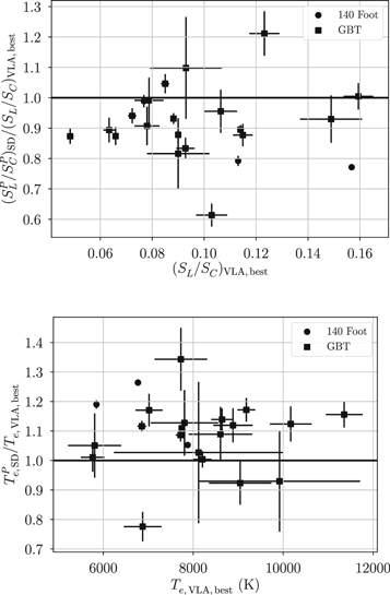
Figure 5. Ratio of single-dish to VLA RRL-to-continuum brightness ratios (top) and electron temperatures (bottom) as a function of the VLA values for the same nebulae as in Figure 4. The weighted mean ratio of the single-dish and VLA RRL-to-continuum brightness ratios is 0.86 ± 0.03 and the weighted mean electron temperature ratio is 1.12 ± 0.03, where the weights are the reciprocal variances in the ratios derived from the fitted Gaussian parameter uncertainties.
Download figure:
Standard image High-resolution imageThe cause of the systematic difference between the single-dish and VLA RRL-to-continuum brightness ratios and electron temperatures is unclear. The difference may be due to a problem with the derivation of the RRL-to-continuum brightness ratio or perhaps due to a fundamental difference in the RRL and/or continuum emission measured by the different telescopes. We know that there are a few issues with how the single-dish RRL-to-continuum ratios are derived. B15 measured the continuum flux densities of their nebulae at νC = 8556 MHz, whereas the average frequency of their observed RRL transitions is  . In the Appendix, we show that the B15 strategy overestimates the true electron temperature by ∼6%. Furthermore, we do not scale the single-dish and VLA RRL-to-continuum brightness ratios to a common frequency because each survey observed similar RRL transitions. The typical VLA
  weighted frequency is within 2% of the B15 average RRL frequency. Neither of these two effects can fully explain the observed 10% difference between the single-dish and VLA RRL-to-continuum brightness ratios.
There are several factors that might affect the measured continuum and/or RRL flux densities: the single-dish continuum flux densities are uncertain due to poor continuum background subtraction; the single-dish telescopes are not pointed at the center of the continuum source during the RRL observation; the VLA is not sensitive to extended emission associated with the H ii region; and/or the VLA is seeing more optically thick gas. (1) The continuum flux densities are the largest source of uncertainty in the single-dish electron temperature derivation (see B15). If the continuum background level is poorly constrained, then the single-dish continuum flux densities will be inaccurate. We limit our analysis to high-continuum QF single-dish nebulae, however, so these problems should be minimal. Furthermore, random errors in the single-dish continuum background levels would not cause the observed systematic difference in single-dish versus interferometric electron temperatures. (2) The single-dish RRL spectra must be measured at the location of the peak continuum brightness. If the telescope is not pointed properly, then the RRL flux densities will be underestimated. This is also not a likely explanation for the discrepancy because B15 peaked on source for their RRL observations. (3) The VLA is not sensitive to diffuse emission. If the source of such emission has a different density and/or temperature, the VLA electron temperatures will differ from the single-dish values. (4) Finally, the nebulae may be optically thick, and/or the compact emission visible to the VLA is more optically thick than the diffuse emission missed by the VLA. Optical depth effects such as these would lead to an underestimation of the VLA continuum flux densities and electron temperatures. Some or all of these issues may be contributing to the remaining 4% discrepancy between the single-dish and VLA RRL-to-continuum brightness ratios.
We wish to use as much data as possible to constrain the metallicity structure of the Galactic disk. Therefore, in subsequent analyses that combine the single-dish and VLA electron temperatures, we multiply the single-dish electron temperatures by 0.9 to accommodate the systematic offset between the VLA and single-dish data.
5.4. Distances
Distances to Galactic H ii regions are derived in three main ways: (1) spectrophotometrically, (2) geometrically, and (3) kinematically. Spectrophotometric distances are only available for optically unobscured nebulae. Since most of the nebulae in our sample are very distant with lines of sight passing through the Galactic plane, we do not consider spectrophotometric distances in this analysis. The extremely fine angular resolution provided by very long baseline interferometry (VLBI) is used to measure the parallaxes and proper motions of masers associated with high-mass star-forming regions (e.g., Reid & Honma 2014). Several hundred maser parallax measurements have been made as part of the Bar and Spiral Structure Legacy (BeSSeL) Survey,8 the Japanese VLBI Exploration of Radio Astrometry (VERA),9 and various European VLBI Network (EVN)10 projects. The vast majority of Galactic H ii regions, however, lack parallax measurements. We must therefore rely on kinematic techniques to derive the distances to nebulae without a geometric distance determination.
Of the 189 Galactic H ii regions in our sample with accurate electron temperature determinations, 46 (24%) have a maser parallax measurement. As in Wenger et al. (2018), we derive the parallax distance and distance uncertainties by Monte Carlo resampling the measured parallax within its uncertainties. We generate 5000 samples of the parallax distance, then we fit a kernel density estimator (KDE) to the distance distribution to calculate a probability distribution function (PDF). The peak of the PDF is the derived parallax distance, and the width of the PDF characterizes the parallax distance uncertainty (see Wenger et al. 2018).
Kinematic distances are computed by measuring the line-of-sight velocity of an object and assuming that object follows some Galactic rotation model (GRM). We use the Wenger et al. (2018) Monte Carlo kinematic distance method and the Reid et al. (2014) GRM to derive the kinematic distances to our sample of Galactic H ii regions. This method computes the distances and distance uncertainties by resampling the observed LSR velocities, the solar motion parameters, which define the LSR, and the GRM parameters to determine the kinematic distance PDFs. Wenger et al. (2018) find that the Monte Carlo kinematic distances are reasonably accurate when compared to the parallax distances for a sample of 75 Galactic high-mass star-forming regions. The median difference between the kinematic and parallax distances for these nebulae is 17% (0.42 kpc).
Within the Solar circle, there exists a kinematic distance ambiguity (KDA). An axisymmetric GRM yields the same LSR velocity at two distances, and additional information must be used to break this degeneracy. The WISE Catalog lists the KDA resolutions (KDAR) for a subset of the known Galactic H ii regions. As in Wenger et al. (2018), we use the WISE Catalog KDARs for nebulae with LSR velocities farther than 20 km s−1 from the tangent point velocity. All nebulae within 20 km s−1 of the tangent point velocity are assigned to the tangent point distance.
Due to line-of-sight velocity crowding, kinematic distances are inaccurate in the direction of the Galactic center and anti-center. Following Wenger et al. (2018), we remove all kinematic distance nebulae located within the zones −15° < ℓ < 15° and 160° < ℓ < 200°. After removing these nebulae, we are left with 121 Galactic H ii regions with kinematic distances. Our final catalog contains 167 nebulae with accurate electron temperatures and either a parallax (46) or kinematic (121) distance. Table 6 lists the relevant distance parameters for each nebulae: the heliocentric distance d; the Galactocentric radius, R; the distance method ("P" for parallax and "K" for kinematic); and the maser parallax observation reference, if any. Nebulae with accurate electron temperatures, without a parallax measurement, and in the direction of the Galactic center/anti-center are also included in this table for completeness. These nebulae are, however, excluded from all subsequent analyses.
5.5. Metallicity Structure
H ii region electron temperatures are a proxy for their nebular metallicities (e.g., Churchwell & Walmsley 1975). The H ii region electron temperature structure across the Galactic disk thus reveals structure in metallicity. Shaver et al. (1983) derived an empirical relationship between H ii region metallicities, determined using optical collisionally excited lines to derive the oxygen and hydrogen column densities, and electron temperatures, determined from RRLs:
where Te is the nebular electron temperature.
We begin our investigation of Galactic chemical structure by measuring the radial electron temperature and metallicity gradients. Figure 6 shows the nebular electron temperature and metallicity gradients using the electron temperatures and Galactocentric radii from Table 6 and metallicities derived using Equation (8). The metallicity uncertainties are determined by propagating the electron temperature uncertainties through Equation (8). We use a robust least-squares routine to fit a linear model to both distributions. The least-squares fit is robust because we dampen the effect of outliers by minimizing a "soft" loss function,  , where z is the squared residuals. This routine does not consider the uncertainties of the data because (1) there are uncertainties in both the dependent and independent variables and (2) the Galactocentric radius uncertainties are asymmetric. Nonetheless, the best-fit linear model to the nebular electron temperature distribution is Te/K = (4345 ± 68) + (374 ± 12)R/kpc, and the best fit for the nebular metallicity distribution is 12+log10(O/H) = (9.148 ± 0.038) − (0.054 ± 0.004)R/kpc. Within the errors, these gradients are consistent with the gradients found by B15 using their "best" distances and Green Bank sample: Te/K ∝ (402 ± 33)R/kpc and 12 + log10(O/H) ∝ (−0.058 ± 0.004)R/kpc.

Figure 6. The nominal radial electron temperature (top) and metallicity (bottom) gradients. The abscissa error bars are the 1σ uncertainties in the parallax or kinematic distances derived from our Monte Carlo distance analysis, and the ordinate error bars are the 1σ uncertainties in the electron temperature or metallicity derived from the continuum and RRL uncertainties. The lines are the robust least-squares linear model fits to the data as defined in the legends.
Download figure:
Standard image High-resolution imageA simple least-squares fitting method cannot account for asymmetric uncertainties in both the abscissas (i.e., Galactocentric radii) and the ordinates (i.e., electron temperatures). Therefore, we estimate the true variance of the linear model by Monte Carlo resampling the data 1000 times. The electron temperatures are drawn from a Gaussian distribution centered at the derived electron temperature and with a width equal to the derived electron temperature uncertainty. The Galactocentric radii are drawn from the parallax or kinematic distance PDFs. For each realization of the data, we fit a robust least-squares linear model. Similar to the Monte Carlo kinematic distance method in Wenger et al. (2018), we estimate the most likely linear model parameters by fitting a KDE to the PDFs of each model parameter. The peak of this KDE is the most likely parameter, and the 1σ confidence interval is derived from the bounds of the PDF such that (1) the PDF evaluated at the lower bound is equal to the PDF evaluated at the upper bound and (2) the integral of the normalized PDF between the bounds is 68.3%. Figures 7 and 8 show, respectively, the most likely linear model parameters derived from this Monte Carlo method and the covariance between the model parameters for the electron temperature and metallicity gradients. The most likely fits are  and
and  . These gradients are within 1σ of the nominal least-squares values, and the asymmetric uncertainties are more accurate given the uncertainties in the derived electron temperatures and distances.
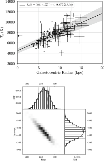
Figure 7. The most likely electron temperature gradient determined by Monte Carlo resampling the derived electron temperatures and Galactocentric radii. The top panel shows the data and the most likely linear model (black line) as defined in the legend. The error bars are the same as in Figure 6. The shaded region represents the range of fits from 1000 Monte Carlo realizations of the data. The bottom panel shows the covariances between the linear model parameters (slope, with units of K kpc−1, and intercept, with units of K). The histograms are the PDFs of the Monte Carlo fit parameters, and the black curves are KDE fits to the PDFs. The solid lines are the peaks of the PDFs (the most likely fit parameters), and the dotted lines represent the 1σ confidence intervals. The dashed lines are the nominal values of the fit parameters derived from the robust least-squares fit to the data (i.e., without Monte Carlo resampling, as in Figure 6).
Download figure:
Standard image High-resolution image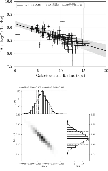
Figure 8. Same as Figure 7 for the radial metallicity gradient. The most likely linear model is defined in the legend. The covariance slope has units of dex kpc−1 and the intercept has units of dex.
Download figure:
Standard image High-resolution imageTo visualize the variations in nebular electron temperature in the Galactic disk, we use kriging to spatially interpolate between discrete nebulae (see also B15). The kriging method computes the average semivariance of the data as a function of the spatial separation between the data points. The average semivariance is measured in many separation bins, known as "lags," and the semivariogram (average semivariance as a function of lag) is fitted with a model. The expected value of the data at any position is derived from this semivariogram model (see Feigelson & Babu 2012).
We compute the nominal kriging map of nebular electron temperatures using the Table 6 electron temperatures and distances. Figure 9 shows this electron temperature map, where we use a linear semivariogram model to interpolate between the discrete H ii region positions. The top panel is the kriging result and the bottom panel is the standard deviation of the kriging interpolation. This standard deviation map characterizes the intrinsic scatter of the data across the Galactic disk. The H ii region points are colored by their electron temperature to highlight the differences between the actual nebular electron temperature and the interpolated value at that position. Figure 10 shows the same kriging results with a linear semivariogram model for the H ii region metallicities. Qualitatively, these figures are similar to the electron temperature and metallicity maps in B15. It is clear from these figures that the radial gradients have a strong dependence on Galactocentric azimuth.
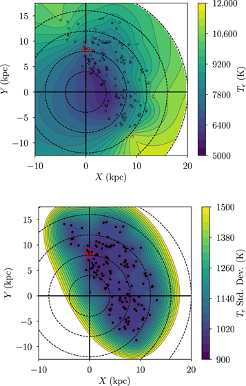
Figure 9. Kriging map of nebular electron temperatures. The top panel shows the kriging interpolation in a face-on view of the Galactic disk. The points are the H ii regions in our sample, colored by their derived electron temperatures. The bottom panel shows the kriging standard deviation. The Galactic Center is located at the origin and the Sun is located at the red cross. The dashed circles are 4, 8, 12, 16, and 20 kpc in radius. White areas are outside R = 20 kpc or have data values beyond the range shown on the color bar.
Download figure:
Standard image High-resolution image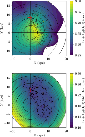
Figure 10. Same as Figure 9 for the nebular metallicities.
Download figure:
Standard image High-resolution imageThese kriging results consider neither the uncertainties in the nebular electron temperatures and metallicities nor the H ii region distance uncertainties. We estimate the most likely kriging map of nebular electron temperatures and metallicities using a Monte Carlo technique in the same way as we determined the most likely radial gradients. We Monte Carlo resample the data within their uncertainties 1000 times, and, for each realization of the data, we generate a kriging map. At each pixel of the kriging map, we construct a PDF of the interpolation values, fit a KDE, and locate the peak and bounds of the KDE. The peak is the most likely kriging value at that position, and the bounds represent the 1σ confidence interval, as before.
Figures 11 and 12 show the most likely kriging interpolation map, most likely standard deviation map, and the upper and lower 1σ confidence interval bound maps for the nebular electron temperatures and metallicities, respectively. The qualitative structure in the Monte Carlo kriging interpolation maps is similar to that in the nominal kriging maps, though the 1σ confidence interval bound maps reveal where the kriging interpolation is ill constrained. For most of the Galactic disk, the most likely kriging values have 1σ bounds ≲500 K in electron temperature and ≲0.8 dex in metallicity. These uncertainties are significantly less than the most likely kriging standard deviations of ∼1000 K and ∼0.25 dex, which suggests that the intrinsic scatter in the nebular electron temperatures and metallicities exceeds the formal uncertainties.
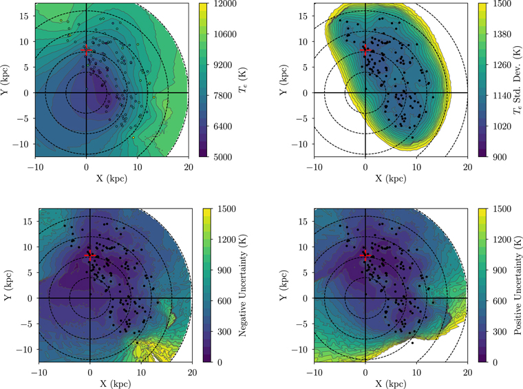
Figure 11. Most likely kriging map of nebular electron temperatures determined by Monte Carlo resampling the derived electron temperatures and distances. Shown are the most likely kriging interpolation values (top left), most likely kriging standard deviation values (top right), lower 1σ bounds (bottom left), and upper 1σ bounds (bottom right) on the kriging interpolation confidence intervals. The features in each plot are the same as in Figure 9.
Download figure:
Standard image High-resolution image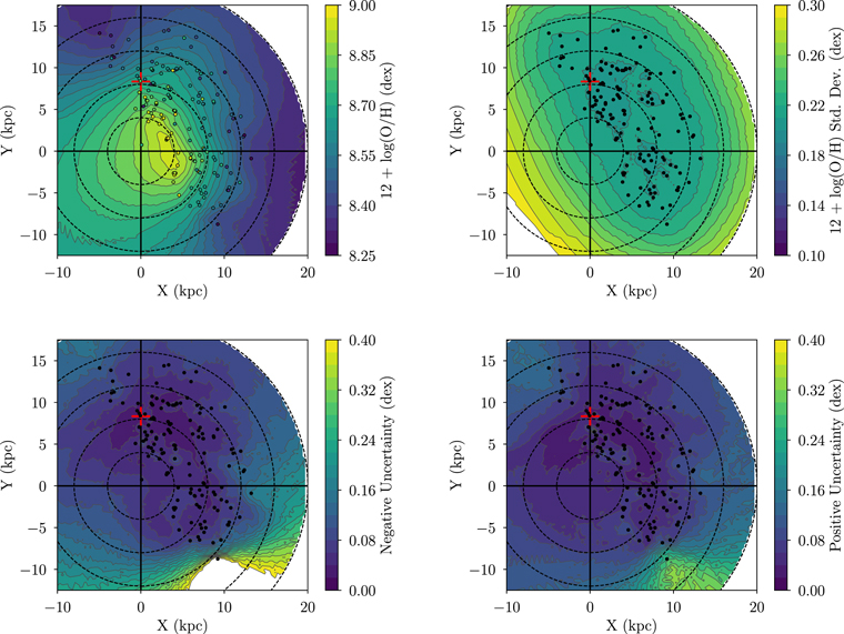
Figure 12. Same as Figure 11 for the nebular metallicities.
Download figure:
Standard image High-resolution image6. Discussion
The radial gradient is the most prominent feature in the metallicity structure of the Galactic disk. Our Monte Carlo analysis of nebular metallicities results in a most likely H ii region oxygen gradient of −0.052 ± 0.004 dex kpc−1. Mollá et al. (2019a) list the oxygen abundance gradients derived from a variety of tracers (see their Table 2). The derived gradients range from about −0.05 dex kpc−1 for H ii regions and Cepheids to about 0 dex kpc−1 for old stellar populations. Our H ii region oxygen gradient is consistent with those found using Cepheids (e.g., −0.0529 ± 0.0083 dex kpc−1 from Korotin et al. 2014), other H ii region samples (e.g., −0.0525 ± 0.0189 dex kpc−1 from Fernández-Martín et al. 2017), and the Mollá et al. (2019a) binned H ii region sample (−0.048 ± 0.005 dex kpc−1).
The large variance in the measured radial metallicity gradients of different tracers is likely due to two primary effects: (1) changes in the metallicity gradient with time and (2) dynamical evolution of stellar populations. The radial gradient as traced by stars is flatter at larger heights above the Galactic midplane (Cheng et al. 2012; Anders et al. 2017). There is evidence that the stellar metallicity gradient also flattens in the inner galaxy (Hayden et al. 2015). These stellar populations are likely older, and thus their metallicity gradient reflects that of a younger Galaxy. Radial migration also plays an important role in stellar metallicity gradients (Sellwood & Binney 2002). The dynamical influence of non-axisymmetric features, like spiral arms and bars, can cause stars to migrate from their birth locations. Some studies have found that radial migration significantly affects the observed stellar metallicity gradients (e.g., Minchev et al. 2013, 2014), whereas others find only an increase in the stellar metallicity dispersion at all Galactocentric radii (e.g., Grand et al. 2014). These effects should have little impact on the H ii region metallicity gradient because these nebulae are very young (≲10 Myr) compared to the dynamical timescale of the Galaxy (∼250 Myr). For example, Grand et al. (2014) use a chemodynamical simulation of a Milky Way-size galaxy to show that, over time, the gas metallicity maintains a low dispersion at all radii, whereas the dispersion of the stellar metallicity increases due to radial migration.
Evidence for azimuthal variations in the radial electron temperature and metallicity gradients has been found in the Milky Way (e.g., B15) and other galaxies (e.g., Ho et al. 2017). Here we expand upon the B15 analysis by using a larger sample of Galactic H ii regions and a more accurate kinematic distance derivation technique. Evidence for azimuthal structure is already apparent in Figures 9–12, and here we test the statistical significance of these azimuthal variations.
To quantify the azimuthal structure in the nebular electron temperature and metallicity radial gradients, we divide the Galaxy into azimuthal bins and compute the radial gradients within each bin. Following B15, we use bins of size 30° in Galactocentric azimuth centered every 5° from −50° to 200°. Using the nebulae in each bin, we make a robust least-squares linear fit to their derived electron temperatures and metallicities as a function of their Galactocentric radii. Figure 13 shows the best-fit linear model slopes as a function of Galactocentric azimuth for the nebular electron temperature and metallicity gradients. Unlike B15, we do not exclude bins with only a few nebulae, nor those with nebulae spanning a small range of Galactocentric radii. The uncertainties in these bins will be correctly determined in the subsequent Monte Carlo analysis. In this simple least-squares analysis, however, the best-fit parameters and their uncertainties are unreliable in sparsely populated bins, such as those below ∼0° and above ∼120°. Nonetheless, we find a similar structure in the electron temperature and metallicity gradient slopes as found by B15. The electron temperature and metallicity slopes vary by a factor of 2 and 3, respectively, between Galactocentric azimuths of ∼20° and ∼100°. These variations are slightly less in magnitude than those found by B15, probably because of our much larger sample size near 100° in Galactocentric azimuth.

Figure 13. Nominal variations in the radial electron temperature (top) and metallicity (bottom) gradients as a function of Galactocentric azimuth. The Galaxy is divided into 30° bins spaced every 5° in Galactocentric azimuth. The points are the slopes of the robust least-squares linear model fit to the data in each bin, and the error bars are the 1σ uncertainties in the fitted slopes. Bins below ∼0° and above ∼120° are sparsely populated and their slopes are unreliable.
Download figure:
Standard image High-resolution imageMultiple sources of uncertainty affect the apparent azimuthal variations shown in Figure 13. These sources include the derived electron temperature uncertainties and the distance uncertainties, which affect both the derived Galactocentric radii and azimuths of the nebulae. To better quantify these sources of uncertainty and to test the statistical significance of the apparent azimuthal variations, we perform yet another Monte Carlo analysis. We Monte Carlo resample the nebular electron temperatures, metallicities, and distances to generate 1000 realizations of the data. As before, the electron temperatures and metallicities are drawn from a Gaussian distribution, whereas the distances are drawn from the parallax or kinematic distance PDFs. For each realization of the data, we fit the radial gradients in each of the several Galactocentric azimuth bins. Finally, we fit a KDE to the linear model parameter PDFs to estimate the most likely parameters and their confidence intervals.
Figure 14 shows the most likely electron temperature and metallicity gradients from our Monte Carlo analysis. The most obvious difference between this and the nominal gradients in Figure 13 is the larger error bars. This Monte Carlo analysis properly accounts for the uncertainties in both the nebular electron temperatures/metallicities and distances, so these error bars more accurately reflect the uncertainties in the gradients within each azimuth bin. Despite the larger uncertainties, the azimuthal variations in the radial gradients remain statistically significant. The electron temperature gradient ranges from ∼250 K kpc−1 at ∼30° to ∼500 K kpc−1 at ∼100°, a factor of ∼2 increase, and the metallicity gradient ranges from about −0.035 dex kpc−1 to about −0.075 dex kpc−1 over the same range, a factor of ∼2 decrease.
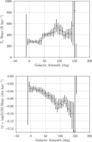
Figure 14. Same as Figure 13 for the most likely gradients derived from our Monte Carlo analysis. The error bars are the 1σ confidence intervals on the most likely slopes.
Download figure:
Standard image High-resolution imageThe derived electron temperatures and metallicities are the largest source of error in the radial gradient determinations. Figure 15 shows the radial metallicity gradients in each Galactocentric azimuth bin where we Monte Carlo resample only the metallicity (top) or only the distances (bottom). The gradient uncertainties are a factor of ∼2 larger when we resample only the metallicities.
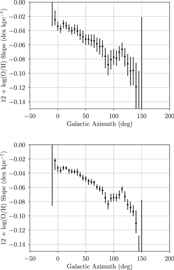
Figure 15. Same as the metallicity gradients in Figure 14, except we only Monte Carlo resample the derived metallicities (top) or distances (bottom).
Download figure:
Standard image High-resolution imageThe azimuthal variations in the metallicity gradient are predicted by some simulations (Di Matteo et al. 2013; Grand et al. 2016). Grand et al. (2016), for example, find azimuthal metallicity structure in the young, thin disk stellar population of a cosmological simulation of a Milky Way analog. The azimuthal variations are induced by the non-axisymmetric peculiar motions near spiral arms, which drives radial migration and a redistribution of metals. The magnitude of the azimuthal variations is ∼0.1 dex in their simulation. If such stellar azimuthal metallicity structure is persistent over long periods of time, the enrichment of the ISM by these stars might explain the observed azimuthal structure in the HII region metallicity distribution. Di Matteo et al. (2013) find a similar magnitude of variation in metallicities as traced by old stars in an N-body simulation. In Figure 16, we show the residuals of the electron temperature and metallicity Monte Carlo kriging maps after subtracting the most likely radial gradients. Excluding the Galactic center and edge of the map, the magnitude of variation in the metallicity residual map is ∼0.1 dex, which is consistent with the Grand et al. (2016) simulation. In the first quadrant, the residual structure between R ∼ 6 kpc and ∼12 kpc is qualitatively similar to the simulated residuals in Grand et al. (2016) and may be evidence for spiral arm induced radial migration in the Milky Way.

Figure 16. Most likely electron temperature (top) and metallicity (bottom) Kriging map residuals. The residuals are determined by subtracting the most likely gradient from the Monte Carlo Kriging maps. The features in each plot are the same as in Figure 9.
Download figure:
Standard image High-resolution image
Recent two-dimensional chemical evolution models also predict azimuthal structure in the gas-phase oxygen abundance. For example, Spitoni et al. (2019) find that density fluctuations due to spiral arms produce oxygen abundance variations on the order of ∼0.1 dex, with the most azimuthal structure apparent at and beyond the corotation radius. The magnitude of these abundance fluctuations decreases with time as the model galaxy becomes well-mixed. This model does not consider stellar migration and enrichment, which, according to the Grand et al. (2016) simulation, are likely important factors. Mollá et al. (2019b) use a 2D chemical evolution code applied to a Milky Way analog to conclude that spiral arms only marginally alter the azimuthal metallicity structure. Their model predicts present-day oxygen abundance variations of ∼0.03 dex increasing to ∼0.1 dex in the outer Galaxy. The oxygen abundance variations are more significant within 1–2 Gyr after spiral arms are introduced in their model.
The nebulae in this study cover only about one-half of the Galactic disk. The Southern H ii Region Discovery Survey (SHRDS; Wenger et al. 2019) is finding hundreds of new H ii regions in the third and fourth Galactic quadrants, and the SHRDS interferometric observations will allow for accurate electron temperature and metallicity derivations. In a future work, we will combine these northern sky nebulae with newly discovered southern sky H ii regions to create a map of H ii region metallicities across the entire Galactic disk. We will use this map to test the chemodynamical evolution simulations by searching for evidence of metallicity structure associated with spiral arms, the Galactic bar, and/or other components of the Milky Way.
7. Summary
We use the VLA to measure the ∼8–10 GHz RRL and radio-continuum flux densities of 82 Galactic H ii regions. We derive the RRL-to-continuum brightness ratio, electron temperature, and metallicity of these nebulae. Including previous single-dish observations, the catalog of Galactic H ii regions with accurate electron temperatures and distances now contains 167 nebulae spanning Galactocentric radii 4–16 kpc and azimuths −20° to 140°.
The distances to Galactic H ii regions are the largest source of uncertainty in previous studies using these nebulae to trace Galactic metallicity structure (e.g., B15). Maser parallax distances have been determined for 46 of our nebulae. For the remainder, we use a novel Monte Carlo kinematic distance technique to determine distances (Wenger et al. 2018). Both the kinematic distances and distance uncertainties to the nebulae in our sample are more accurate than in the B15 study. In this work, the RRL-to-continuum brightness ratio uncertainties are about twice as important as the distance uncertainties.
Using a Monte Carlo analysis, we derive the most likely Milky Way radial electron temperature and metallicity gradients as  and
and  , respectively. This metallicity gradient is consistent with previous H ii region studies (e.g., B15) and young stellar tracers, such as Cepheids (e.g., Korotin et al. 2014). We generate maps of the electron temperature and metallicity structure of the Galactic disk using a Monte Carlo kriging analysis. These maps reveal significant azimuthal variations in the Galaxy's metallicity structure. The radial metallicity gradient varies by a factor of ∼2 (∼0.04 dex kpc−1) between Galactocentric azimuths of ∼30° and ∼100°. We find non-axisymmetric spatial metallicity variations on the order of ∼0.1 dex, which is consistent with the Grand et al. (2016) chemodynamical simulation. These variations may be evidence for radial migration and metal mixing induced by the Milky Way's spiral arms.
The Southern H ii Region Discovery Survey (Wenger et al. 2019) will add hundreds of nebulae with electron temperature and metallicity derivations to the third and fourth Galactic quadrants. With H ii region coverage across the entire Galactic disk, we will investigate the association between the Milky Way's metallicity structure and the locations of spiral arms. Such structure is a test of chemodynamical simulations and can be directly compared to extragalactic systems.
We thank the anonymous reviewer for their constructive feedback on this manuscript. T.V.W. is supported by the NSF through the Grote Reber Fellowship Program administered by Associated Universities, Inc./National Radio Astronomy Observatory, the D.N. Batten Foundation Fellowship from the Jefferson Scholars Foundation, the Mars Foundation Fellowship from the Achievement Rewards for College Scientists Foundation, and the Virginia Space Grant Consortium. L.D.A. is supported in part by NSF grant AST-1516021. T.M.B. is supported in part by NSF grant AST-1714688.
The National Radio Astronomy Observatory is a facility of the National Science Foundation operated under cooperative agreement by Associated Universities, Inc.
Facility: VLA. -
Software: Astropy (Astropy Collaboration et al. 2013), CASA (McMullin et al. 2007), KDUtils (Wenger et al. 2017), Matplotlib (Hunter 2007), NumPy & SciPy (van der Walt et al. 2011), PyKrige (Murphy 2014), Python (https://www.python.org/), WISP (Wenger 2018).
Appendix: Electron Temperature Derivations
Here we derive the relationship between the nebular electron temperature, hydrogen radio recombination line (RRL) brightness, and radio-continuum brightness of an H ii region. This derivation relies on several assumptions: (1) the nebula is homogeneous, isothermal, and in LTE; (2) the nebula is optically thin in both radio-continuum and RRL emission; (3) the nebula is composed solely of ionized hydrogen and singly ionized helium; and (4) the RRL and continuum brightness are measured with the same telescope in the Raleigh–Jeans limit.
The free–free radio-continuum absorption coefficient of an isothermal plasma is
where Te is the electron temperature, ν is the observed frequency, ni is the ion number density, and ne is the electron number density (Oster 1961). Altenhoff et al. (1960) approximate the absorption coefficient as
which is accurate within 10% for 100 MHz < ν < 35 GHz and 5000 K < Te < 12000 K (Mezger & Henderson 1967). The free–free optical depth is the integral of this absorption coefficient along the line of sight,  . In a homogeneous medium with line-of-sight depth l, the optical depth simplifies to τC(ν) = kCl.
The LTE hydrogen RRL absorption coefficient for the transition from principle quantum state m to n is
where νL is the RRL rest frequency, χn is the energy required to ionize the atom from state n, fnm is the oscillator strength of the m to n transition, ϕν(ν) is the normalized line profile with inverse frequency units, np is the hydrogen number density, h is the Planck constant, k is the Boltzmann constant, e is the electron charge, me is the electron mass, and c is the speed of light (Brocklehurst & Seaton 1972; Balser 1995). The Rydberg formula determines the transition frequency between state m and n:

where Z is the effective nuclear charge and R is the Rydberg constant. For hydrogen, Z = 1 and  , where
  is the Rydberg constant for an infinite mass and mp is the proton mass. If we let Δn = m − n, then the hydrogen transition frequencies are

For the low Δn transitions in the radio regime (e.g., H109α), Δn ≪ n and

Substituting these frequencies into Equation (11), and assuming that we are observing in the Rayleigh–Jeans limit χn ≪ kTe, the LTE RRL absorption coefficient becomes
Evaluating the constants and moving to astrophysically relevant units, this equation becomes
The RRL optical depth is the integral of this absorption coefficient along the line of sight, which is  for a homogeneous medium.
In an optically thin medium in LTE, the specific intensity of some emission with optical depth τ is Iν ≃ Bν(T)τ, where Bν(T) is the Planck function at some temperature T. Assuming the RRL and continuum emission originate in the same volume of homogeneous, isothermal gas with electron temperature, Te, the RRL-to-continuum specific intensity ratio at νL is
For a Gaussian line profile with FWHM line width Δν,
and

Using Equation (19) in (17), we find
If the nebulae is composed of only hydrogen and singly ionized helium, then
where  is the singly ionized helium number density and
  is the ratio of singly ionized helium to hydrogen by number. We use the Doppler equation to convert the FWHM line width from frequency to velocity units:
where ΔV is the FWHM line width in velocity units. The RRL-to-continuum specific intensity ratio at νL is thus
The expression (fnmΔn/n) is not a strong function of n for Δn = 1 hydrogen RRLs. For example, (fnmΔn/n) = 0.19435, 0.19395, and 0.19363 for Δn = 1 and n = 80, 90, and 100, respectively, using the oscillator strengths from Menzel (1968). This variation is less than 0.3% across these Hnα transitions, so we adopt the H90α oscillator strength to simplify the RRL-to-continuum specific intensity equation as

Solving for the electron temperature, we find
A.1. Single-dish Observations
Single-dish telescopes measure intensity in units of antenna temperature, TA. In the absence of atmospheric attenuation, the antenna temperature is related to the brightness temperature distribution, TB(θ), by

where ηb is the telescope beam efficiency, Ωb is the telescope main beam solid angle, f(θ) is the telescope beam pattern, and the integral is the convolution of the source brightness distribution with the telescope beam (Mezger & Henderson 1967). For a Gaussian beam with HPBW θb, the beam pattern is ![$f(\theta )=\exp [-4\mathrm{ln}(2){\theta }^{2}/{\theta }_{b}^{2}]$](https://content.cld.iop.org/journals/0004-637X/887/2/114/revision1/apjab53d3ieqn379.gif) and the beam solid angle is
and the beam solid angle is  . Similarly, if the source brightness distribution is Gaussian with amplitude TB and half-power width θs, then the source brightness temperature distribution is
 ![${T}_{B}(\theta )={T}_{B}\exp [-4\mathrm{ln}(2){\theta }^{2}/{\theta }_{s}^{2}]$](https://content.cld.iop.org/journals/0004-637X/887/2/114/revision1/apjab53d3ieqn381.gif) . In astronomy, θ is typically very small,
. In astronomy, θ is typically very small,  , and the integral in Equation (26) is
where we use  . The antenna temperature is thus

For a resolved source, θs ≫ θb and TA ≃ ηbTB. For an unresolved source, θs ≪ θb and  .
.
Brightness temperature is defined as

where Iν is the specific intensity. For an optically thin medium, Iν = Bν(T)τ, where T is the blackbody temperature of the emission and τ is the optical depth. In the Rayleigh–Jeans limit, the brightness temperature is simply

Substituting Equation (30) into (28), we find

If the RRL and continuum antenna temperatures are measured with the same telescope and at the same frequency, and if both sources of emission originate from the same volume of homogeneous and isothermal gas with electron temperature Te, Equation (24) is trivially
where TC(νL) and TL(νL) are the continuum and RRL antenna temperatures measured at the RRL frequency νL, respectively. Equation (25) becomes
A.2. Averaging Single-dish RRLs
In Galactic H ii region surveys, we average multiple RRL transitions to increase the RRL signal-to-noise ratio. Each RRL transition is an independent measurement of the nebular electron temperature, so the electron temperature derived from many RRL-to-continuum antenna temperature measurements is
assuming that adjacent RRL transitions have similar FWHM line widths in velocity units (e.g., Balser et al. 2011). Previous single-dish RRL studies have used different strategies for averaging RRL transitions. Balser et al. (2011, 2015), for example, scale each RRL antenna temperature to account for the variations in telescope beam size with frequency, then average the rescaled RRL spectra. They measure the continuum antenna temperature at one frequency within the RRL frequency range, then take the ratio of the average RRL antenna temperatures to this continuum temperature. This strategy is an approximation to Equation (34).
Here we compute the difference between the true electron temperature and the Balser et al. (2011, 2015) approximation using multiple RRL transitions. From Equation (34), the factor we need to derive is
where Te ∝ Xtrue and Xtrue is the only variable in Equation (34) that depends on the RRL transition. Balser et al. (2011, 2015) approximate this factor as

where νC is the observed continuum frequency and  is the RRL antenna temperature corrected for the variation of telescope beam size with frequency. They rescale the observed RRL antenna temperature, TL(νL), using

where θb is the HPBW at νL, and  is the HPBW at νC, and θs is the half-power width of the source. The observed source brightness distribution is the convolution of the actual source brightness and the telescope beam. With the assumption that the telescope beam and source brightness distribution are Gaussian, the convolution is also a Gaussian with half-power width
  . Balser et al. (2011, 2015) measure the source half-power width at νC, which is
  . The true, deconvolved source size is
  , and the rescaled antenna temperature in terms of observables is
For a point source,  and
and ![${T}_{L}^{* }({\nu }_{L})\simeq {T}_{L}({\nu }_{L}){[{\theta }_{b}^{2}/({\theta }_{b}^{* })}^{2}]$](https://content.cld.iop.org/journals/0004-637X/887/2/114/revision1/apjab53d3ieqn391.gif) , whereas if the source is very resolved,
, whereas if the source is very resolved,  and
and  .
.
Using Equations (16), (19), and (22), the line center LTE optical depth of the ith RRL transition is
where we have assumed  for a homogeneous medium with an LTE absorption coefficient
  and a line-of-sight depth l. The antenna temperature of this transition is
and the rescaled RRL antenna temperature is
The average rescaled RRL antenna temperature of several RRL transitions is

assuming that the RRLs have similar FWHM line widths in velocity units.
From Equation (10), the continuum optical depth at frequency νC is
where, again, we have assumed that the medium is homogeneous. The continuum antenna temperature is
Substituting Equations (42) and (44) into the Balser et al. (2011, 2015) approximation of X, we find
The ratio of the X approximation and Xtrue is
As a sanity check on this expression, if the RRL and continuum antenna temperatures are measured at only one RRL frequency, then  and this ratio is unity. Balser et al. (2015) measured the continuum antenna temperature at νC = 8.556 GHz and the RRL antenna temperature for 6 Hnα transitions (H87α to H93α, excluding H90α). The average RRL frequency is
  , but Balser et al. (2015) use
  . With these values, the X ratio is

Therefore, Balser et al. (2015) and other studies that average the same RRL transitions and observe the same continuum frequency will overestimate the derived electron temperatures by ∼5.7%.
Quireza et al. (2006a, 2006b) use different RRL transitions and calibration strategies to derive electron temperatures. In their C ii survey, they observe H91α and H92α. They assume both transitions have the same antenna temperature in the bright H ii region W3, and they use this assumption to calibrate H92α relative to H91α. From Equation (40), this calibration factor is

W3 is unresolved in their survey, so  . Using
  for a Gaussian beam, this factor becomes

Therefore, the average RRL antenna temperature in their surveys is
The continuum antenna temperature at νC is given by Equation (44), and the Quireza et al. (2006a, 2006b) X is
The ratio of this X approximation to Xtrue is
Quireza et al. (2006a, 2006b) did not account for the variation in telescope beam size in their analysis. Therefore, their ratio X/Xtrue has a dependence on the source size. In the limit that the source is unresolved at all frequencies,  . For Gaussian beams with θ2∝ ν−2, the ratio in this limit becomes

Using the RRL frequencies, νC = 8.665 GHz, and  , which is what Quireza et al. (2006a, 2006b) use, we find

For unresolved sources, Quireza et al. (2006a, 2006b) correctly calculate the electron temperatures in their C ii survey. In the resolved case,  and
and
Therefore, the Quireza et al. (2006b) electron temperatures for the C ii survey nebulae are underestimated by up to 5% depending on the source morphology.
In their 3He survey, Quireza et al. (2006a, 2006b) only observe the H91α transition. The X ratio for this survey is simpler:
with limits
and
Quireza et al. (2006b) underestimate their electron temperatures by up to 2% in their 3He survey.
In Table 7, we list the X/Xtrue factors for the Quireza et al. (2006a, 2006b), Balser et al. (2011), and B15 single-dish studies. For each survey, we list the author; the observed RRL transitions; the observed continuum frequency; the average RRL frequency they used in the electron temperature equation; and the X/Xtrue factor.
Table 7. Single-dish Electron Temperature Corrections
| Author | RRLs | νC |
 a
a
|
X/Xtrue |
|---|---|---|---|---|
| GHz | GHz | |||
| Quireza et al. (2006a, 2006b) C ii Survey | H91α;H92α | 8.665 | 8.585 | 0.956 to 1.0 |
| Quireza et al. (2006a, 2006b) 3He Survey | H91α | 8.665 | 8.585 | 0.983 to 1.0 |
| Balser et al. (2011, 2015) | H87α to H93α | 8.665 | 9.0 | 1.057 |
Note.
aAverage RRL frequency used by the author, which is not the actual average RRL frequency.Download table as: ASCIITypeset image
A.3. Interferometer Observations
Interferometers measure intensity in units of flux density per synthesized beam, S, which is related to brightness temperature, TB, by the Rayleigh–Jeans law:

If the RRL and continuum flux densities are measured at the same frequency, with the same telescope, and with the same synthesized beam size, the RRL-to-continuum flux density ratio and electron temperature are given by Equations (24) and (25), respectively, where IC is the continuum flux density and IL is the RRL flux density.
A.4. Averaging Interferometer RRLs
An important difference between interferometric observations and single-dish observations is that interferometers measure the RRL and continuum emission simultaneously. At each RRL frequency, we measure the RRL flux density and continuum flux density with the same synthesized beam. If the source is homogeneous and isothermal, we can ignore all effects of the varying beam size.
In our VLA survey analysis, we extract spectra from our data cubes in two ways: from the pixel of brightest continuum emission, such that the spectrum has units of flux density per beam, or from the sum of all pixels within a region, such that the spectrum has units of flux density. We average these spectra weighted by the continuum brightness and rms noise in the line-free regions, so our interferometric X factor is
where SC and SL are the continuum and RRL brightness or flux density, respectively, and  indicates a weighted average. If we assume that the spectral rms noise is the same in each RRL transition, then the weighted average values are simply


From Equations (10) and (59), the continuum brightness at the ith RRL frequency is
for a homogeneous nebula with depth l. The RRL frequency is the only factor that depends on RRL transition, so
and
Using Equations (16) and (59), the LTE brightness of the ith RRL is
for a homogeneous medium with depth l. The average RRL brightness is
The average RRL frequency is
so the interferometric X approximation simplifies to
The ratio of this approximation to Xtrue is
We observe the seven RRL transitions from H87α to H93α. Our X factor ratio is thus

Our strategy for averaging multiple RRL transitions to compute electron temperatures is accurate.