


Abstract
Atomic oxygen (O0) plays a critical role in determining the structure of photon-dominated regions (PDRs), but reliable modeling of its emission has been hampered by the high optical depth of the 63 μm fine structure line and complexities in the excitation of the relevant fine structure levels. We discuss here radiation produced by collisional excitation of the submillimeter fine structure lines of atomic oxygen ([O I]) using recent calculations of rates for collisions with atomic and molecular hydrogen. We employ the Molpop–CEP code to include the effects of optical thickness in slab models that are characterized by uniform oxygen abundance, hydrogen density, and kinetic temperature. The particular spontaneous decay rates and collisional excitation rates connecting the three O0 fine structure levels result in population inversion of the upper, 145 μm transition. The effects of trapping are rigorously included and are reflected in the resulting line profiles that exhibit prominent self-absorption even with uniform physical conditions. We present figures for analyzing the two fine structure lines based on the intensity of the 63 μm line and the 145 μm/63 μm line ratio. For the clouds considered, the results for line intensities and line ratios are modestly different from those obtained with a large-velocity-gradient model, but the ability to calculate line profiles is an additional powerful tool. Comparison of the model results with observed line profiles suggests that cloud models with varying physical conditions are required to optimally utilize [O I] fine structure line emission to trace the energetics of PDR regions and the feedback from massive, young stars.
Export citation and abstract BibTeX RIS
1. Introduction
The energy from star formation put into a neighboring photon-dominated region (PDR) controls subsequent star formation in its surroundings, and it is thus critical to have reliable information on PDR structure and kinematics, as well as on the radiation from them, in order to understand how feedback from massive, young stars determines galactic evolution. Oxygen is the third most abundant element in the universe, and in a wide variety of astronomical environments it is found in neutral atomic form (O0). Fine structure line emission ([O I]) from atomic oxygen is the dominant coolant of warm PDRs and plays a key role in determining their structure and luminosity. The 63 μm line can be the most powerful far-infrared line in galaxies having relatively warm PDRs heated by massive star formation (Malhotra et al. 2001). Accurate analysis of [O I] emission has been hampered by the evident high optical depth of the 63 μm line and by the lack of a convenient and efficient code that can model radiative transfer in clouds with varying conditions along the line of sight.
The two lines at wavelengths 63.2 and 145.5 μm are widely used to analyze conditions in interstellar clouds and galaxies (e.g., Poglitsch et al. 1995; Oberst et al. 2011; Díaz-Santos et al. 2017). Almost all observations of these lines have been made with relatively low spectral resolution, so line profiles could not be determined. Several studies of regions of massive star formation carried with modest spectral resolution suggested [O I] absorption by foreground material (Poglitsch et al. 1996; Herrmann et al. 1997), but were not conclusive.
Observed line intensities and line profiles from some of the earliest detections (Stacey et al. 1983, 1993; Boreiko & Betz 1996) in giant molecular clouds suggested that the 63 μm line is often optically thick. This conclusion was consistent with straightforward single-component modeling that accompanied the observational results. Observational studies of regions of less-massive star formation and thus potentially with smaller gradients in conditions were surprising in terms of yielding extremely large values of line ratio I(145)μm/I(63)μm ≃ 0.4 (Caux et al. 1999; Liseau et al. 1999). These and the following papers cited reported fluxes (erg s−1 cm−2) and ratios. We have converted these to intensities (erg s−1 cm−2 sr−1) and calculated ratios assuming that beams are uniformly filled.
Their analyses indicated large optical depths in the 63 μm line, but the modeling with uniform physical conditions did not result in lower O0 column densities; Caux et al. (1999) concluded that N(O0)/N(CO) = 50, far greater than predicted by any chemical models. Saraceno et al. (1998) observed more than 70 pre-main-sequence objects with Infrared Space Observatory (ISO) and found higher I(145)μm/I(63)μm ratios than could readily be explained by models. These authors concluded that the explanation is colder gas associated with the source, rather than unrelated foreground material along the line of sight. Liseau et al. (2006) analyzed archival ISO data on many young stellar objects observed in both [O I] lines and suggested that tenuous foreground gas is absorbing the 63 μm line, making quantitative conclusions difficult. Nisini et al. (2015) observed jets in six young stellar objects, again finding relatively high I(145)μm/I(63)μm ratios. The jet emission lines are very broad (δv between 125 and 184  ), so the suggestion of foreground absorption being responsible for high I(145)μm/I(63)μm ratios seems problematic. Their conclusion that H2 molecule collisions are an order of magnitude less effective than H atoms in achieving a particular line ratio differs sharply from what we find with the more modern collision rate coefficients discussed in Section 2.
The upGREAT instrument on the Stratospheric Observatory for Infrared Astronomy (SOFIA) now offers the possibility of velocity-resolved spectroscopy of both [O I] lines, and recent observations (e.g., Leurini et al. 2015; Schneider et al. 2018; Mookerjea et al. 2019) have confirmed earlier suggestions (above references and Boreiko & Betz 1996) that optical depth effects are significant. [O I] spectra from SOFIA as well as those anticipated from the upcoming balloon mission GUSTO (https://www.nasa.gov/press-release/nasa-selects-mission-to-study-churning-chaos-in-our-milky-way-and-beyond) suggest that modeling tools that can predict line profiles as well as intensities will be very valuable. Anticipated new far-infrared spectroscopic observatories, including the ESA/JAXA M-Class Mission SPICA (Roelfsema et al. 2018) and the Origins Space Telescope proposed to the 2020 Decadal Survey (Leisawitz et al. 2018), will cover these spectral lines, albeit with a velocity resolution insufficient for detailed line profile studies of Galactic sources.
This paper is intended to take a step in this direction by presenting model results obtained with the Molpop–CEP statistical equilibrium/radiative transfer code (Elitzur & Asensio Ramos 2006; Asensio Ramos & Elitzur 2018). This code overcomes a major limitation of the commonly used large velocity gradient (LVG) model (e.g., Goldreich & Kwan 1974), which assumes that as a result of a large spatial velocity gradient, the radiative transfer is purely local, so that different portions of the spectral line are produced in different portions of the cloud. While satisfactory for many purposes and extremely computationally efficient, the LVG approximation is not able to model regions with very different physical conditions having the same velocity. Such regions are thus able to exchange photons, resulting in, for example, self-absorption features. Radiative transfer models that can handle interchange of photons more generally (e.g., Rybicki & Hummer 1991) are much more computationally demanding than LVG. The Molpop–Cep code achieves accuracy comparable to state-of-the-art accelerated Λ-iteration (ALI) codes while being orders of magnitude more rapid for cases with the many zones required to handle high optical depths (see discussion in Elitzur & Asensio Ramos 2006).
This paper is organized as follows. In Section 2 we discuss the fine-structure energy level structure of [O I] and recent results on collisions with molecular and atomic hydrogen, and in Section 2.2 we describe the behavior of the lines in the optically thin and optically thick limits. In Section 3 we present representative line profiles for a cloud with uniform conditions, and in Section 4 we give results for line intensities and line ratios as a function of H2 density, kinetic temperature, and atomic oxygen column density.
2. [O i] Fine Structure Levels and Collisional Excitation
The oxygen atom in its ground electronic state has three fine structure levels. As shown in Figure 1, they are inverted in energy, with the  level having the highest energy and the 3P2 the lowest. The two allowed transitions are also indicated; the 3P0–3P2 transition has a spontaneous decay rate approximately a factor of 105 smaller and can be ignored for astronomical purposes. Information about the three fine structure transitions is given in Table 1. The collisional deexcitation rate coefficients are for a kinetic temperature of 100 K from Lique et al. (2018). These authors calculate the rate coefficients for H2 in the J = 1 and J = 0 states individually, as well as the rates for collisions with H and He.
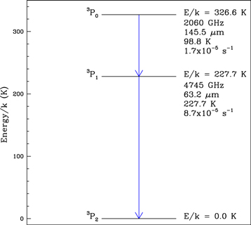
Figure 1. Fine structure levels and transitions of atomic oxygen in the ground electronic state with equivalent temperature of each level indicated. For each transition, we include the frequency, wavelength, equivalent transition temperature, and spontaneous decay rate. The vastly weaker and in practice unimportant 3P0 → 3P2 transition is not shown. See Table 1.
Download figure:
Standard image High-resolution imageThe deexcitation rates for [O I] by collisions with atomic hydrogen are (as discussed by Lique et al. 2018) significantly smaller, by factors of 3 to 6, than those calculated previously by Abrahamsson et al. (2007). The Lique et al. (2018) deexcitation rate coefficients for collisions with H2 are 2–4 times larger than those calculated by Monteiro & Flower (1987) for collisions with He producing the same transitions.
The deexcitation rates for collisions with H2 are within a factor of 2 of those calculated by Jaquet et al. (1992) for deexcitation by ortho- and para-H2. The values given here for collisions with H2 are the average of the rates for the two spin states. The two rate coefficients for collisions to the ground state are comparable, and the rates for H2 in J = 1 and J = 0 differ by less than 20%. The value for the 3P0–3P1 transition is approximately a factor of 50 smaller than the other two deexcitation rate coefficients, due to an approximate selection rule that forbids this transition (see discussion in Lique et al. 2018 with references to earlier treatments, including Monteiro & Flower 1987). This rate is a factor of ∼3 larger for H2 in J = 1 than in J = 0, but the small magnitudes make using the average value of H2 in J = 0 and J = 1 at all temperatures an acceptable approximation.
The major difference between collisions with H2 and with H is the absence of the dramatically smaller 3P0–3P1 deexcitation rate coefficients for collisions with atoms, due to the presence of an indirect channel (Lique et al. 2018). Given the composition of the regions where the abundance of [O I] is expected to be appreciable, we focus on collisions with molecular hydrogen.
The rate equations for a three-level system presented and discussed in Goldsmith et al. (2015) can be applied to the [O I] fine structure lines, but with the caution that the ordering by total angular momentum is inverted for [O I] compared to that for [N ii]. The relevant expressions are given in the Appendix.
2.1. Relationships
Observations of the [O I] fine structure lines have been carried out by low-resolution spectrometers, such as PACS on Herschel (Poglitsch et al. 2010), and with high-spectral-resolution instruments that resolve line profiles (Risacher et al. 2016). While there is obviously significant additional information in the velocity-resolved spectra, current and future instrumentation, especially for extragalactic observations, will continue to employ the most sensitive spectrometers, which will not resolve the emission. In this paper, we give results for both types of observations, as well as some relationships for conversion between the two generally employed ways to present data.
Velocity-resolved spectroscopy has largely been carried out with single-mode diffraction-limited systems. The system is characterized by its effective area Ae, which applies to radiation coming from the direction of maximum sensitivity (the optical axis or boresight direction). The response to radiation coming from other directions is described by the normalized power pattern Pn, which is a function of the angle away from the boresight. Note that Pn has value unity for radiation incident from the boresight direction. We let such a system observe a source that has unpolarized specific intensity Iν (units of, e.g., erg s−1 cm−2 sr−1 Hz−1), which is a function of angle  . Within a frequency interval δν at frequency ν, over which I is assumed to be constant, the power received in a single polarization with the telescope boresight at angle Ω is

If the source is uniform over the angular extent covered by Pn (or close to this limit), the expression simplifies to

The integral in the above expression is the antenna solid angle, ΩA. From the antenna theorem (e.g., Goldsmith 2002), for any single-mode diffraction-limited antenna, AeΩA = λ2. This gives us

The power received from the antenna in a single-mode system defines the antenna temperature, TA, through

This gives the relationship for conversion between antenna temperature and specific intensity:

Here, TA is a function of frequency, varying across the spectral line being observed, although this is generally not expressed explicitly in such expressions. Equation (5) allows conversion between antenna temperature and specific intensity for resolved spectral lines.
If we do not resolve the line, then what we observe is the antenna temperature integrated over frequency, which is related to the intensity  through

Although the natural units for integrated antenna temperature are K Hz, it usually is expressed in units of K km s−1, and we write

Table 2 gives values for the constants relating antenna temperature and intensity for the two [O I] fine structure transitions. An approximate value for the antenna temperature can be obtained from the intensity by assuming a simple line shape and line width Δv. Then, dividing the value of  obtained using the fourth column of Table 2 by the assumed Δv yields the peak antenna temperature.
2.2. Limiting Cases
It is valuable to consider some limiting cases of excitation of the [O I] fine structure lines. For this purpose, we use analytic expressions that give insight into the behavior of the system. Equivalent expressions have been previously developed for three level systems in articles (e.g., Liseau et al. 2006) and books (Draine 2011), but we start here from basic principles for completeness and clarity.
Here, and in what follows, we use the superscript 63 to denote the 3P1–3P2 transition having a wavelength ≃63 μm, and 145 to denote the higher-lying 3P0–3P1 transition with λ ≃ 145 μm.
We denote the collision rate coefficient from level i to level j as Rij, which has units cm−3 s−1. The rate coefficients are obtained by integrating the cross sections over the velocity distribution of the colliding particles. The Rij values here are denoted γij by Spitzer (1978) and qij by Osterbrock (1989). For collisions with species k (here hydrogen atoms or hydrogen molecules), the collision rate is Cij = Rijn(k), having units s−1. The rate of collisional transitions per unit volume is equal to ni(O)n(k)Rij = ni(O)Cij.
2.2.1. Optically Thin Subthermal Emission
Subthermal excitation occurs when the downward collision rates are much smaller than competing radiative rates. In this limit, the collisional processes that enter into the rate equations for the level populations (density of oxygen in level i, ni(O)) are exclusively upward (excitation) collisions, and we obtain


and
where nt is the total volume density of O0 atoms. These results depend on the relative magnitudes of the different collision rate coefficients. Note that C23 does not appear, and that the ratio n3/n2 is independent of density in the subthermal limit, while the ratio n2/n1 is proportional to the collision rate and thus the density. From Table 1, the ratio A21/A32 is equal to 5.1, and with the statistical weights of level i, gi = 2i + 1 for i = 1, 2, and 3, the upward collision rates (for kinetic temperature 100 K) are C12 = 1.1 × 10⁻¹¹ n(H2) s−1 and C13 = 1.0 × 10⁻¹² n(H2) s−1. We then find the population ratios n2/n1 = 1.4 × 10⁻⁷ n(H2) and  .
.
Table 1. [O I] Fine Structure Transitions and Collisional Parameters
| Transition | Frequencya | Wavelength |
 /k /k |
Aulb | Rul(H)c | Rul(H2)c |
|---|---|---|---|---|---|---|
| (GHz) | (μm) | (K) | (s−1) | (10−10 cm3 s−1) | (10−10 cm3 s−1) | |
| 3P0–3P1 | 2060.069 | 145.53 | 326.6 | 1.7 × 10⁻⁵ | 0.84 | .0291 |
| 3P1–3P2 | 4744.777 | 63.18 | 227.7 | 8.7 × 10⁻⁵ | 1.12 | 1.74 |
| 3P0–3P2 | 6804.847 | 44.06 | 326.6 | 1.4 × 10⁻¹⁰ | 0.76 | 1.36 |
Notes.
aFrom Zink et al. (1991); these values supersede those of Saykally & Evenson (1979). bFrom Fischer & Saha (1983). There are slight differences among different calculations and references; see Baluja & Zeippen (1988). cAt kinetic temperature 100 K.Download table as: ASCIITypeset image
The excitation temperature describes the relative populations per unit statistical weight and for transition from level u to level l is defined as
where  = ΔEul/k is the equivalent temperature of the transition with ΔE the energy difference between the upper and lower levels. This yields the subthermal limits for the excitation temperatures (for collisions with H2 at a kinetic temperature of 100 K) Tex145 = −387 K, and for a density of 103 cm−3, Tex63 = 27 K.
The results from Molpop–CEP with an O0 column density sufficiently small that optical depths are far less than unity are shown in Figure 2. The 63 μm transition is well behaved, with Tex63 rising smoothly toward the 100 K kinetic temperature. Here, Tex63 for n(H2) = 103 cm−3 is again 27 K. The figure includes results for collisions with atomic hydrogen (Lique et al. 2018). The O–H rates being a few times smaller than those for O–H2 collisions results in slightly lower values of Tex at intermediate densities.

Figure 2. Excitation temperature of the two [O I] fine structure lines for a kinetic temperature of 100 K. The results of collisions with H2 are indicated by the triangles and with H by the squares. The values of Tex145 for n(H2) ≤ 104 cm−3 are negative, and their magnitude is plotted. For n(H) in this range, the values of  are greater than 400 K and so do not appear on this plot.
Download figure:
Standard image High-resolution imageFrom the full calculation, at densities n(H) ≤ 102 cm−3, Tex145 = −333 K, close to the approximate value of −387 K given above and representing a very small difference in the level populations. The population inversion of the 145 μm transition (noted previously with earlier collision rate coefficients by, e.g., Liseau et al. 2006 and with more recent coefficients by Lique et al. 2018) is evident for densities n(H2) ≤ 105 cm−3. For this range of densities, the rapid depopulation of the lower (3P1) level by spontaneous decay to the ground state overwhelms the combination of radiative decay from the upper (3P0) level and collisional population of the lower level by collisions from the ground (3P2) state.
The presence of the population inversion is due to the relative magnitude of the rates of populating the levels by collisions compared to depopulation by spontaneous emission. The relative collision rate coefficients depend only on the kinetic temperature. As discussed above, at 100 K the ratio n3/n2 = 0.43, which is larger than the ratio of the statistical weights g3/g2 = 0.33. In order to eliminate the population inversion, we require that C12/C13 (equal to 10.4 at 100 K) be greater than or equal to 14.6. At a kinetic temperature of 50 K, for example, this ratio is ≃28, because the rate from the ground state to the second excited state is reduced more by the low kinetic temperature than is the rate from the ground state to the first excited state. The result is indeed no population inversion, but rather a modestly superthermal excitation with Tex145 ≃ 150 K.
The inversion potentially provides amplification, but the column density of atomic oxygen in plausibly sized regions of this low density and the suppression of the inversion by the buildup of intensity at the frequency of the transition together prevent the development of any anomalously strong line intensities. For densities greater than 105 cm−3, collisional deexcitation becomes significant and Equation (8) is no longer valid.
The intensity of optically thin emission in a transition from level u to level l is given by

The ratio of intensities of two transitions can yield valuable information. Assuming that the ratio of the column densities is equal to that of the volume densities, we find for optically thin emission from [O I] that

In the subthermal limit, we use Equation (8) and obtain

The line intensity ratio I145/I63 for optically thin emission increases as the kinetic temperature increases in the subthermal (low excitation rate) limit, growing by a factor of ≃5 as the kinetic temperature goes from 50 to 400 K. This temperature dependence is a reflection of the greater energy requirement for the primary excitation path for the 145 μm line, C13, compared to that for the 63 μm line, C12. If the volume density can be constrained to ≤105 cm−3 and the atomic oxygen column density to ≤1017 cm−2, the line ratio can be a useful probe of the temperature in the PDR.
For a kinetic temperature of 100 K, the ratio of the intensities is

The intensity can be converted to peak or integrated intensity through Equations (5) to (7). The antenna temperature ratio of the two [O I] transitions, if both are optically thin and have equal line widths, can be written as

In the subthermal limit, we find from Equations (8) and (16) that

and for low H2 densities at a kinetic temperature of 100 K, we find
The primary dependence on kinetic temperature is through the difference in upper state energies as included in Equation (17), with weaker dependence from the temperature dependence of the collision rates themselves.
2.3. Optical Depth
The optical depth of a spectral line is proportional to its line profile function ϕ(ν) describing its frequency dependence, normalized such that  . The optical depth τ is given by

where Nl and Nu are the lower- and upper-level column densities, respectively, and Blu and Bul are the upward and downward stimulated emission coefficients. Assuming a Gaussian line profile with dispersion σ and FWHM line width Δν = 1.67σ, we find that the line profile function at the line center is  . Using the line width expressed in
  , we obtain

Using the relationship between upward and downward stimulated emission coefficients and the relationship between the B and A coefficients, we find
where N is the total column density of the species and fl is the fraction in the lower level of the transition.
We define a maximum line center optical depth, τ0, by taking the FHWM line width equal to 1  , a lower-level column density of 1 cm−2, and highly subthermal excitation so that
  ≫ 1, allowing us to neglect the exponential term. This yields

and

Table 3 gives values of τ0 and fl for local thermodynamic equilibrium (LTE) at different temperatures. Even with the assumption of LTE, the fractional population of the lower level of the 63 μm line (3P2 level) is not far from unity, and that for the lower level of the 145 μm line (3P1 level) is between 0.02 and 0.07.
PDRs are material subjected to ultraviolet and visible radiation that cannot ionize hydrogen, but deposits energy that both heats the gas and dust and controls the chemical composition of these regions (Tielens & Hollenbach 1985). Figure 3 shows aspects of a PDR relevant to [O I] emission, generated using the Meudon PDR code (Le Petit et al. 2006). In a PDR exposed to a radiation field enhanced by a factor of 104 relative to the standard interstellar radiation field (which is easily attained in regions of massive star formation) and density of 104 cm−3, oxygen is essentially all in atomic form for visual extinctions Av ≤ 3.5 and is still over 30% atomic for Av = 10 mag.
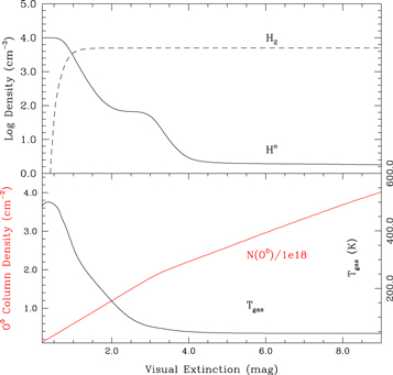
Figure 3. Structure of PDR illuminated by a radiation field enhanced by a factor of 104 relative to a standard interstellar radiation field from the left-hand side (Av = 0). The hydrogen nucleus density is 104 cm−3 throughout, and the total extinction through the slab is 10 magnitudes. Upper panel: densities of atomic and molecular hydrogen as a function of visual extinction. Lower panel: gas temperature and atomic oxygen column density as a function of visual extinction. The decrease in the slope of  vs. Av at 3.5 mag results from CO rather than O0 being the dominant form of oxygen at larger extinctions.
Download figure:
Standard image High-resolution imageThe transition from atomic to molecular hydrogen with the parameters of the present model occurs at Av ≃ 0.9 mag. At a density of 104 cm−3, the kinetic temperature is somewhat over 500 K for Av ≤ 0.4 mag, drops to 200 K at Av = 1.6 mag, and continues to drop beyond that point. Even in the higher temperature portion of this PDR, the fraction of oxygen in the 3P1 level is only a few percent, and far less than this when the temperature drops below 100 K. The total column density of atomic oxygen in the PDR is on the order of 3 × 1018 cm−2. We thus can take fl = 1 for the 63 μm line and fl = 0.01 for the 145 μm line. From Table 3 and Equation (23) we find that, for a line width of 5  and the above parameters, τ145 (ν0) = 0.04 and τ63 (ν0) = 3. It is readily apparent that the 63 μm line can be significantly optically thick, while the 145 μm line will almost certainly be optically thin.
2.4. [O i] Absorption
The optically thick [O I] emission from a PDR source can easily result in "self-absorbed" line profiles. This terminology is somewhat arbitrary given the lack of detailed models, but implies that there is gas along the line of sight with lower excitation than that of the PDR itself. This is readily seen in molecules having high critical densities (e.g., H2O; Ashby et al. 2000). However, since these features are typically only a few  wide, they are not readily discerned in most existing [O I] data, which were obtained with far lower velocity resolution. At low resolution, the absorption of the combined source line and continuum emission can result in an almost pure absorption feature (Baluteau et al. 1997; Kraemer et al. 1998a, 1998b).1
There is a large body of observational data on [O I] 63 μm absorption by "foreground" clouds; the distinction here is that the velocity of the absorption is typically offset from that of the emission (Keene et al. 1999; Vastel et al. 2000). Absorption by unrelated foreground clouds along the line of sight readily occurs against relatively distant sources, and the velocity offsets due to Galactic rotation may result in multiple components blending together to provide a very broad absorption "trough" (Lis et al. 2001; Vastel et al. 2002; Wiesemeyer et al. 2016). As suggested by the entries in Table 3, the 63 μm line will be in absorption, while the emission from the source in the 145 μm line is relatively unaffected by the foreground gas, due to the very low opacity of this line (González-Alfonso et al. 2012).
The situation for external galaxies is complicated by the possible presence of both source and foreground absorption, with the two being confused by the velocity spread of the sources within the telescope beams employed. It is thus difficult to assess the importance of opacity in the 63 μm line, as might be expected from Galactic sources. Most of the galaxies analyzed by Fernández-Ontiveros et al. (2016), for example, have I145/I63 between 0.06 and 0.2. The lower values (up to 0.08) may be produced by optically thin emission, but only at kinetic temperatures greater than 250 K. For higher values of I145/I63, the 63 μm line must be optically thick, with I145/I63 ≃ 0.6 for Arp 220 indicative of enormous opacity in the lower [O I] transition.
2.5. Transition to the Optically Thick Regime
The radiative trapping resulting from a transition being optically thick can be thought of as reducing the spontaneous emission rate, thus bringing the excitation closer to LTE. This is often relevant for the 63 μm transition, which is subthermally excited for a wide range of densities up to n(H2) ≃ 106 cm−3 (see discussion in Section 2.6). Figure 4 shows this behavior for atomic oxygen in a region with n(H2) = 103 K. As shown by the red curve in the lower panel, the optical depth of the 63 μm transition increases almost linearly with Oo column density and reaches a value of 10 for N(Oo) = 4 × 1018 cm−2. At this point, the excitation temperature indicated by the red curve in the upper panel has increased appreciably above the value ≃27 K produced by collisional excitation alone.

Figure 4. Lower panel: optical depth of the [O I] transitions for kinetic temperature 100 K, density n(H2) 103 cm−3, and FWHM line width 1.67  as a function of the atomic oxygen column density. The optical depth τ145 (blue) is negative for N(O0) ≤ 1017 cm−2, and these values of the optical depth are multiplied by −105. Note that τ145 is positive for N(O0) ≥ 1017 cm−2. The optical depth τ63 is shown in red. Upper panel: excitation temperatures of the two transitions. Values at the center and edge of the slab are denoted C and E, respectively. The values of
  displayed are divided by 2, and positive values are shown only for column densities at which
  /2 ≤ 100 K.
Download figure:
Standard image High-resolution imageThe upper panel of Figure 4 shows an additional radiative effect. In this implementation of the Molpop–CEP program, there is no systematic velocity shift through the slab of material being modeled. Thus, the oxygen atoms in the center of the slab are exposed to a stronger radiation field at a frequency of 4475 GHz than are the atoms at its edge. The excitation temperature at the center of the slab (denoted C) is significantly greater than that at the edge (denoted E). This difference increases throughout the range of optical depths included here (up to ≃200), but for sufficient oxygen column density (greater than included here), the transition becomes thermalized throughout.
The situation for the 145 μm transition is more complex, as the adopted density of 103 cm−3 produces a population inversion (negative excitation temperature) in the optically thin limit. As the column density increases, so does τ145, but its magnitude is very small, ≤10−5. When N(Oo) reaches 1017 cm−2, the excitation temperature switches to being positive but very large, indicating essentially equal populations in the upper and lower levels. For higher column densities, Tex145 drops, indicating a reduction in the ratio n3/n2. This is not due to the trapping in the 145 μm line, for which the optical depth is very small, ≃10−5–10−2. Rather, the trapping in the 63 μm line effectively reduces its spontaneous decay rate A21, which in turn reduces the the ratio n3/n2 given by Equation (8), and hence Tex145.
We can gain a feeling for this effect by assuming that the reduction in the A coefficient is given by the escape probability β = (1 − exp − τ)/τ ≃ 1/τ for τ ≫ 1. Then for τ63 = 10, βA21/A32 is reduced to 0.51 from its optically thin value of 5.1. The result from Equations (8) and (11) is that Tex145 ≃ 50 K. This is intermediate between the C and E values in Figure 4. Note that the value of Tex145 drops to values below 30 K as a consequence of this effect. Only for oxygen column densities greater than ∼1020 cm−3 does τ145 become sufficiently large that the trapping in this transition begins to drive the excitation temperature up toward the kinetic temperature. The conclusion is that for extended low-density regions with atomic oxygen column densities between 1018 cm−2 and as high as a few ×1020 cm−2, the 145 μm transition can have an excitation temperature below that of the 63 μm transition, with both lines being optically thick.
2.6. Critical Density
The critical density is defined as the density of colliding partners that makes the downward collision rate equal to the spontaneous decay rate, so

As discussed by Goldsmith et al. (2015), in a two-level system, this makes the ratio of upper- to lower-level populations equal to one-half of the value in LTE at the kinetic temperature. Using the definition of excitation temperature (Equation (11)), we define the critical excitation temperature, Texc, as that resulting from a density equal to the critical density. In general,

and from the definition of the critical density, we obtain

From Table 1, the two-level critical density for the 63 μm [O I] line is nc = 5.0 × 105 cm−3, and from the above, Texc = 77 K. From Figure 2, we see that the full calculation gives very close to this same value. The two-level and full calculations agree, due to the relatively low fractional population of the upper 3P0 level and the unimportance of collisions involving that level in determining the properties of the lower 3P1–3P2 63 μm transition.
The situation for the 145 μm line is more complex because there is a population inversion at low densities, so the excitation temperature approaches the kinetic temperature from above as the hydrogen density increases and we reach thermalization. For collisions with H2, the unusually low collisional deexcitation rate coefficient (Table 1) gives a very large value of nc = 5.8 × 106 cm−3. At this density, the excitation temperature of the 145 μm line is only ≃10 K greater than the kinetic temperature. Thus, taking the critical density as defined by Equation (24) gives an unrealistically high value for the H2 density required to bring the excitation temperature close to the kinetic temperature, as collisional pathways other than 3P0–3P1 dominate.
For collisions with atomic hydrogen, the 3P0–3P1 deexcitation rate coefficient has a more typical value, and nc(H0) = 2 × 105 cm−3. From the full calculation, Texc is several times the kinetic temperature at this density, but is dropping rapidly toward the kinetic temperature as the density increases and we approach LTE. For both collision partners, the critical density for the 145 μm line has limited usefulness. Table 4 gives the values of the critical densities for the two [O I] fine structure transitions and collisions with H and H2. The values for collisions with Ho are a factor of ≃2 larger than those given by Fernández-Ontiveros et al. (2016).
2.7. Optically Thin Thermalized Emission
We can use Equation (13) with the LTE value of the density ratio

to obtain

which gives

Figure 5 shows the variation of line intensity ratio as a function of molecular hydrogen density for four values of the kinetic temperature. The behavior for these is largely similar, with I145/I63 dropping by approximately a factor of 4 as the density increases and the excitation changes from subthermal to thermalized. The temperature dependence in the subthermal limit is given in Equation (14), somewhat different than that given in the thermalized limit by Equation (28). In the latter case, the ratio increases as the kinetic temperature increases, due to the higher energy of the upper level of the 145 μm transition, but is independent of the temperature dependence of the collision rates, which do enter for subthermal excitation.

Figure 5. Ratio of intensity of 145–63 μm [O I] transitions as a function of hydrogen density for four values of kinetic temperature. The triangle symbols denote excitation by collisions with molecular hydrogen. The open square symbols for 400 K denote excitation by collisions with atomic hydrogen. There is only a very small difference in the intensity ratio produced by the two collision partners.
Download figure:
Standard image High-resolution imageFor 400 K kinetic temperature, we show in Figure 5 the results for collisions with atomic hydrogen as well as molecular hydrogen. Only a small difference can be discerned for low densities, at which the excitation is subthermal, while for higher densities, the two collision partners yield an identical ratio as the transitions are thermalized. This is quite different from the conclusion of Nisini et al. (2015), who found an order of magnitude or more difference in density to obtain a given intensity ratio when considering collisions with H2 and Ho. This is presumably a result of different collision rate coefficients; those employed by Nisini et al. (2015) were not specified.
2.7.1. Optically Thick Thermalized Emission
In this limit, the antenna temperature is just that of a blackbody at the kinetic temperature Tk:

The ratio of the antenna temperatures of the two [O I] transitions in this limit is

For a kinetic temperature of 100 K, TA145 = 58.6 K while TA63 = 26.0 K, and their ratio is

This high value is a reflection of the greater departure from the Rayleigh–Jeans limit of the shorter wavelength transition. In consequence, the ratio approaches unity for Tk ≥ 250 K, but can become very large for kinetic temperatures appreciably less than 150 K.
3. Line Profiles
The profile of a spectral line can provide information about the line-of-sight variations in physical conditions if there are large-scale velocity gradients through the region of interest. The optical depth has a strong influence on what we can discern in terms of source structure. Optically thin emission plus velocity shifts encode the information about physical conditions into the velocity dependence of the signal. Optically thick emission without large-scale velocity shifts hides from us more distant portions of gas along the line of sight, but even if the emission is optically thick, we can gain some information, such as about the temperature. Optically thick emission can also function as a background source against which lower-excitation foreground gas can be seen in absorption.
Modeling the emergent line spectrum requires following the emission and absorption of photons of different frequencies as they propagate through the cloud. The Molpop–CEP program carries this out, without making any assumptions about the magnitude of velocity gradients (as does the large velocity gradient or LVG model). Photons of a given frequency can be absorbed or can stimulate emission, or can be added to by spontaneous emission, from any point in the cloud. To calculate accurately the line profile, we do have to input the physical conditions as a function of position in the cloud, which is here taken as a slab, with variations only along the line-of-sight coordinate. Doing this can be complex, and there is a real issue in terms of uniqueness in terms of inversion of the observed line profile to determine the source structure. The enormous information content of spectrally resolved observations nevertheless makes this a critical tool for really determining the physical parameters and their variation within a source.
The present paper does not attempt to build a detailed source model (as has been done by, e.g., Schneider et al. 2018). Rather, we give a few examples that indicate the variety of behaviors that can be expected even for a uniform slab model of an [O I] source, and to connect them to the discussion of general behavior given above. We present the results for line profiles in units of antenna temperature, but these can be easily converted to specific intensity through Equation (5) and the values given in Table 2.
Table 2. Conversion Factors
| Transition | ΔE/k | TA/Iν |

|
|---|---|---|---|
| (K) | (K/erg s−1 cm−2 sr−1 Hz−1) | (K km s−1/erg s−1 cm−2 sr−1) | |
| 145 | 98.8 | 7.67 × 10¹¹ | 1.12 × 10⁵ |
| 63 | 227.7 | 1.45 × 10¹¹ | 9.13 × 10³ |
Download table as: ASCIITypeset image
When both transitions are optically thin, the excitation temperature is purely a result of collisional excitation and is uniform throughout the slab. However, when the atomic oxygen column density increases so that the 63 μm line becomes optically thick, radiative trapping starts to affect the level populations and the excitation temperature. Since the cloud modeled here has no large-scale velocity gradient, this first occurs at the center of the cloud, where the effect of the optical depth is greatest.
Figure 6 shows the behavior of the excitation temperature as a function of position within the slab having N(Oo) = 1019 cm−2 and FWHM line width 1.67  , resulting in optical depths of 25–30 for the 63 μm transition and 0.2–1.5 for the 145 μm transition. We thus see significant variation in the excitation temperatures as a function of position in the slab for the two lower volume densities. The 63 μm line with no trapping has T63ex = 27 K (see Figure 2), but as seen in Figure 6, this has been increased to 50 K in the center of the slab, but drops to 39 K at the slab edge. Similar behavior occurs for n(H2) = 105 cm−3, but starting from a purely collisionally produced excitation temperature of 56 K (lower than that seen even in the outermost zone included in Figure 6 due to the radiation from the interior of the cloud).

Figure 6. Variation of excitation of [O I] 63 μm (red) and 145 μm (blue) lines in a uniform slab with Tk = 100 K, N(Oo) = 1019 cm−2, and Gaussian line profile with FWHM = 1.67  for three values of the molecular hydrogen volume density indicated.
Download figure:
Standard image High-resolution imageThe 145 μm line is inverted (T145ex = −339 K) by collisions for n(H2) = 103 cm−3 and superthermal (T145ex = 1550 K) for n(H2) = 105 cm−3 (see Figure 2). The optical depth, τ63 = 30, results in the relatively low excitation temperature T145ex = 30 K in the slab center (see discussion in Section 2.5), which rises as one moves toward the edges of the slab. For lower N(Oo), T145ex rises to above the kinetic temperature and becomes negative at the boundary of the slab. For n(H2) = 107 cm−3, both transitions are nearly thermalized by collisions alone, which is reflected in the minimal variation in excitation temperature throughout the slab.
Figure 7 shows the line profiles for the two [O I] fine structure lines for four values of the atomic oxygen column density. The kinetic temperature is 100 K, the H2 density is 107 cm−3, and the FWHM line width is 1.67  in all cases. For the lowest column density, both lines are optically thin (τ63 = 0.22), and we see nearly Gaussian line profiles. The ratio of peak antenna temperature is
  , very close to the ratio from Equations (16) and (27) for quasi-thermalized excitation.

Figure 7. Line profiles of [O I] 63 μm (red) and 145 μm (blue) emission from a uniform slab with Tk = 250 K, n(H2) = 107 cm−3, and Gaussian line profile with FWHM = 1.67  .
.
Download figure:
Standard image High-resolution imageAs the column density increases, we see that the 63 μm line becomes flat-topped due to saturation for N(Oo) = 1019 cm−2. For this and higher column densities, the peak antenna temperature of the 145 μm line is greater than that of the 63 μm line, due to the departure from the Rayleigh–Jeans limit discussed in Section 2.7.1. While the largest column density N(Oo) = 1020 cm−2 is not widespread, it can be found in massive PDRs (Goicoechea et al. 2015), and it illustrates the limit of a uniform cloud with both transitions thermalized and optically thick.
Figure 8 illustrates the more complex line profiles that can result when the density (and hence the collision rate) alone is insufficient to thermalize the transitions. In this case, with n(H2) = 104 cm−3 and Tk = 100 K, both transitions are, in the absence of trapping, subthermally excited. When the column density reaches 1018 cm−2, the fractional population of the 3P2 state, the lower level of the 63 μm transition, is larger than it is in LTE at Tk = 250 K, so the optical depth is larger, producing the slightly flat-topped appearance.

Figure 8. Line profiles of [O I] 63 μm (red) and 145 μm (blue) emission from a uniform slab with Tk = 100 K, n(H2) = 104 cm−3, and Gaussian line profile with FWHM = 1.67  .
.
Download figure:
Standard image High-resolution imageFor N(Oo) = 1019 cm−2, we see for the first time clear evidence of the importance of radiative trapping and the effect of coupling the radiation from different regions within the slab. Under these conditions, the excitation temperature of the 63 μm line is 79 K in the center of the two-sided slab, but drops to ≤60 K in the outer 5% of the slab. Since the total optical depth through the slab of the line is 28, the outer 5% corresponds to optical depth ≃1. Thus, the antenna temperature at the line center reflects the lower value resulting from purely collisional excitation, while moving into the line wings, one sees deeper into the cloud where the radiative trapping increases the excitation temperature. There is sufficient opacity in the 63 μm line to result in higher antenna temperatures at velocities offset by ±1.5  than at line center.
The 145 μm line has a total optical depth of 0.9, but the radiative trapping here is having the effect, discussed earlier, of suppressing the population inversion produced by collisions. The result is that the excitation temperature T145ex is 44 K at the center of the slab, but is 50–60 K at the edge of the slab where the trapping is less. For N(Oo) = 1019 cm−2, the line profile is close to Gaussian as the optical depth is modest.
For the large column density N(O0) = 1020 cm−2, both transitions are optically thick. The 63 μm line profile is similar to that for a column density an order of magnitude lower, but the central depression is wider because of the larger (τ63 = 260) optical depth. The 145 μm line profile in this situation is similar to that of the shorter-wavelength line because the excitation temperature is 75 K in the center of the slab but only 56 K at the slab edge, with a total optical depth of 16 resulting again in a centrally depressed profile. The behavior of T145ex as a function of column density is shown in Figure 4; for n(H2) = 104 cm−3, its behavior is similar to that for n(H2) = 103 cm−3 illustrated, with the excitation temperature being driven to very low values by trapping of the 63 μm line, and with T145ex increasing toward the center of the slab, where trapping enhances the radiation field at the frequency of the 145 μm transition.
4. Results
The results from models of uniform slabs depend on numerous parameters and can be presented in many ways. The overwhelming majority of data on [O I] fine structure lines to date has been obtained with systems having relatively low spectral resolution that do not resolve the line profiles. Such systems continue to be available (FORCAST on SOFIA) and will possibly be a major source of data in the future (SPICA). With this in mind, we first present some results for line intensities, even though the output from Molpop–CEP always provides the spectral line profiles.
4.1. Line Intensities
We first show results in terms of line intensities for four kinetic temperatures, with the intensity of the 63 μm line and the ratio of the intensity of the 145 μm line to that of the 63 μm line as a function of O0 column density, for specified values of the volume density, n(H2).
The intensity of the 63 μm line (lower panels of Figures 9–12) increases monotonically with O0 column density and volume density. This line is quite optically thick (τ ≥ 3) for N(O0) ≥ 1018 cm−2 (Table 3) and densities below the critical density (Table 4). The emitted intensity continues to increase even though the line is optically thick because collisional deexcitation is unimportant compared to spontaneous decay, and the emission is effectively optically thin (e.g., Goldsmith et al. 2012). At volume densities for which collisional deexcitation is important and the excitation temperature is comparable to the equivalent temperature of the transition, the line intensity saturates for N(O0) ≥ 1018 cm−2, at which point the emission is thermalized and optically thick.

Figure 9. Lower panel: intensity of 63 μm [O I] line as a function of the atomic oxygen column density, N(O0), from a slab having a kinetic temperature equal to 50 K. The FWHM velocity dispersion in the slab is 1.67  . The curves are for different values of the H2 volume density, with the lowest curve for n(H2) = 100 cm−3, and increasing in logarithmic steps of 0.5 dex. Curves with
  , 3.0, and 5.0 are shown in red, with values indicated. Upper panel: logarithm of the ratio of intensity of the two [O I] fine structure lines.
Download figure:
Standard image High-resolution image
Figure 10. Lower panel: as Figure 9 but for kinetic temperature 100 K. Upper panel: as Figure 9 but for Tk = 100 K with the ratio plotted on a linear scale.
Download figure:
Standard image High-resolution image
Figure 11. As Figure 10 but for Tk = 250 K.
Download figure:
Standard image High-resolution image
Figure 12. As Figure 10 but for Tk = 400 K.
Download figure:
Standard image High-resolution imageTable 3. Maximum Line Center Optical Depth and Lower-level Fractional Populations for [O I] Fine Structure Transitions
| Transition | τ0 | fl | |||
|---|---|---|---|---|---|
| T(K) | |||||
| 50 | 100 | 250 | 400 | ||
| 145 | 6.52 × 10⁻¹⁸ | 6.4 × 10⁻³ | 5.8 × 10⁻² | 1.9 × 10⁻² | 2.4 × 10⁻¹ |
| 63 | 4.92 × 10⁻¹⁸ | 9.9 × 10⁻¹ | 9.4 × 10⁻¹ | 7.7 × 10⁻¹ | 7.0 × 10⁻¹ |
Download table as: ASCIITypeset image
Table 4. Critical Densities for [O I] Fine Structure Transitions
| Transition | nc(H2) | nc(H) |
|---|---|---|
| (cm−3) | (cm−3) | |
| 145 | 5.8 × 10⁶ | 2.0 × 10⁵ |
| 63 | 5.0 × 10⁵ | 7.8 × 10⁵ |
Download table as: ASCIITypeset image
The behavior of the line intensity ratio, shown in the upper panels of Figures 9 through 12, was discussed in Section 2.2. The temperature dependence of I145/I63 is similar in the thermalized and subthermal limits. We here see that the dependence on atomic oxygen column density is more complex. The density dependence in the high-column-density limit is inverted compared to that in the low-column-density limit. This is because at low volume densities, the ratio is "anomalously" high because of the peculiar combination of spontaneous emission rates and collision rate coefficients discussed in Section 2.2.1. As the collision rate increases, this ratio is lowered to that characteristic of LTE.
At high column densities, radiation trapping in the optically thick 63 μm line reduces the population of the uppermost 3P0 level and thus the  ratio. The relatively low line intensity ratio at high volume densities and low column densities is increased by the trapping resulting from increased column density. As the trapping increases, the excitation temperature of the 63 μm line begins to rise toward the kinetic temperature, while that of the 145 μm line first drops to quite low values (see Figure 4) but then also increases. The result is that, for a narrow range of column densities, the line ratio is almost independent of volume density. For higher column densities, the intensity ratio increases with increasing volume density up to a maximum value and then drops for higher n(H2). This is seen most clearly for Tk = 400 K.
The ratio of the antenna temperatures, as discussed in Section 2.7.1 and described by Equation (31), is converging to a single value independent of n(H2) and N(Oo). The behavior of the intensity ratio is not so easily calculated, due to the different line broadening due to different optical depths of the two transitions (see, e.g., Figure 7). The beginnings of this trend are seen especially clearly in the right-hand side of Figure 12 for Tk = 400 K.
4.2. Comparison with Other Models and Analysis of Observations
4.2.1. Molpop–CEP Output and Comparison with Results from LVG Calculation
The intensities of the [O I] fine structure lines alone can be presented in many different ways; we here give results in one format that is in effect complementary to that used previously. With only two observed quantities (two line intensities or one intensity and one intensity ratio), we cannot uniquely solve for the three key parameters: O0 column density, H2 density, and kinetic temperature. Here, we fix the kinetic temperature and show the results in I(63 μm)–I(145 μm)/I(63 μm) space for different H2 densities and O0 column densities. Figures 13–15 show the results for H2 densities equal to 103, 104, and 105 cm−3, respectively.

Figure 13. [O I] 63 μm line intensity—[O I] 145 μm/63 μm intensity ratio diagram for H2 density equal to 103 cm−3. The four colored curves are for the four kinetic temperatures indicated. The points on each curve denote the atomic oxygen column density in steps of 0.25 dex. The square box on each curve denotes column density N(O0) = 1018 cm−2. The black curve is the output from the RADEX LVG code for a kinetic temperature of 100 K. The O0 column density ranges from 1.00 × 1014 cm−2 to 1.78 × 1021 cm−2 in steps of 0.25 dex. The black diamonds are the results from Oberst et al. (2011).
Download figure:
Standard image High-resolution image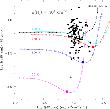
Figure 14. As Figure 13 but for H2 density equal to 104 cm−3.
Download figure:
Standard image High-resolution image
Figure 15. As Figure 13 but for H2 density equal to 105 cm−3.
Download figure:
Standard image High-resolution image
In each figure, we plot the line intensity ratio versus the 63 μm line intensity at a fixed kinetic temperature for different atomic oxygen column densities. The points on each curve denote O0 column densities increasing in steps of 100.25 = 1.78, with the large squares indicating N = 1 × 1018 cm−2.
The black curves show the results from the RADEX LVG code (van der Tak et al. 2007) for a kinetic temperature of 100 K. These curves are generally similar in form to those from Molpop–CEP, but have significantly higher line ratios for the same 63 μm line intensities at the same temperature. The RADEX calculation utilizes older deexcitation rate coefficients included in that program's database that result in higher line ratios, due to the relatively larger excitation rate to the upper, 3P0, level of the triplet. The RADEX results thus mimic the results from Molpop–CEP at higher kinetic temperatures, conditions which also enhance the rate of collisions producing a 3P2 → 3P0 transition.
4.2.2. Comparison with PDR Models
The Molpop–CEP results can only be compared approximately with those from model PDR calculations such as those presented by Kaufman et al. (1999), inasmuch as the latter models a slab heated by an external UV field. Thus, while the density is uniform, the temperature drops substantially as we move inward from the surface. The form of the hydrogen is calculated based on a photochemical model, so it varies from an atomic form at the surface exposed to UV to largely molecular at extinctions ≥1 mag.
For a density of 104 cm−3, Kaufman et al. (1999) determine a surface temperature of 100 K for G0 = 102, log I(63 μm) = −3.4, and log I(145 μm)/I(63 μm) = −1.33. This is close to the value we obtain here for the same density, N(O0) = 1.8 × 1017 cm−2, and T = 250 K. The ratio I(145 μm)/I(63 μm) increases with kinetic temperature for subthermal excitation, as discussed in Section 2.2.1 and illustrated in Figure 5. The gas temperature in the PDR model deceases from its surface value of 100 K, so the higher temperature required for the Molpop–CEP uniform-temperature slab compared to the PDR model cannot be a consequence of the temperature structure in the latter. The difference is likely a combination of the different collision rate coefficients and the change from molecular to atomic hydrogen as one moves toward the illuminated surface of the PDR.
4.2.3. Comparison with Observations of the Carina Nebula and Presence of Foreground Absorption
Figures 13–15 include intensities and intensity ratios from Oberst et al. (2011). The data presented in that paper included the [O I] observations of Mizutani et al. (2004), who observed both [O I] transitions in the central portion of the Carina Nebula. These observations did not resolve the lines spectrally, but having both transitions observed systematically offers a valuable point for evaluating the modeling tool described here. Mizutani et al. (2004) noted some positions with very high values of I(145 μm)/I(63 μm), extending up to 0.09. While details of their modeling are limited, they concluded that these values can only be obtained for very high temperatures, consistent with Kaufman et al. (1999) and with the results presented here. Our modeling does not extend to the required ≃1000 K temperatures, but Mizutani et al. (2004) claim these are excluded in any case by the ratio of [C ii] to [O I].
An alternative explanation of these high ratios is that they are due to a reduction in the 63 μm intensity that is due to absorption by lower-excitation foreground material (see, e.g., Saraceno et al. 1998). If we consider 50 K material having density 104 cm−3 (either a low-density portion of the PDR or unrelated foreground material), the excitation temperature of the 63 μm line will be about 26 K (see Figure 2 for Tk = 100 K), and the fraction of atomic oxygen in the 3P1 state ≃10−4. Consequently, the optical depth of the 145 μm line will be dramatically less than that of the 63 μm line. Using Equation (23) and values of τ0 given in Table 3, for N(O0) = 6.4 × 1017 cm−2 and Δv = 5  , τ63 = 0.65, while τ145 ≃ 10−4. Consider as the "background source" a position with relatively strong PDR emission such as those observed by Mizutani et al. (2004) and Oberst et al. (2011), with I63 = 1 × 10⁻⁴ erg s−1 cm−2 sr−1 and I145/I63 = 0.044. With the above foreground optical depths for the two [O I] transitions, we see that the 63 μm intensity is reduced by a factor of ≃2 (including the very modest emission from the foreground cloud), while that of the 145 μm line is essentially unaffected. The result is that the intensity ratio is increased from 0.044 to 0.085.
Thus, a pair of line intensities that would be very difficult to fit now suggest PDR emission that is satisfactorily represented by a PDR with Tk ≃ 250 K, n(H2) ≃ 105 cm−3, and N(O0) ≃ 1 × 1016 cm−2, with the less-excited, moderately optically thick foreground component discussed above. These parameters are not unique, but indicate that correcting for the foreground absorption can result in reasonable parameters for the atomic oxygen emission from the PDR instead of the observational results being problematic. The presence of foreground absorption can possibly be traced by the line profile, and this is another important aspect in which velocity-resolved spectra can be extremely valuable.
5. Conclusions
We have presented results from a step in developing more complete and realistic models with which to interpret observations of the submillimeter fine structure transitions of atomic oxygen. While observations of the [O I] 63 μm line, especially those that spectrally resolve the emission, have been limited, and those of the 145 μm line even less plentiful, observations of this atom have already proven to be powerful diagnostics of Galactic PDRs and widely employed as a tracer of star formation in Galactic sources and external galaxies. One significant development has been to go beyond the upper frequency limit of the HIFI instrument on Herschel (de Graauw et al. 2010), which now enables SOFIA observations of both [O I] lines by upGREAT (Risacher et al. 2016).
Observation of velocity-resolved spectra will give significantly more ability to interpret the complex structure of the PDR regions producing emission, which are often accompanied by less-excited [O I] associated with the emission region that produces self-absorption features, and also unrelated foreground [O I] responsible for additional absorption features. We have thus utilized the Molpop–CEP code to study [O I] emission. This radiative transfer and statistical equilibrium code accounts for photon trapping and produces emergent line profiles that can readily be compared with observations. We here present results from a uniform slab model that can be used as a first approximation in analyzing observations.
We present some salient features of the collisional excitation of the [O I] fine structure levels based on recently published quantum calculations by Lique et al. (2018). We confirm earlier analyses that found population inversion of the shorter-wavelength 145 μm transition, and we find that radiative trapping of the much more optically thick lower 63 μm transition suppresses this inversion. We find that the 63 μm line is often optically thick and that trapping increases its excitation temperature if the density is below the critical density, 5 × 105 cm−3 and 8 × 105 cm−3 for H2 and H0, respectively. The less-excited [O I] at the surface of the slab readily produces self-absorption features in the 63 μm line profiles, similar to those often observed.
However, the absorption features produced by a cloud modeled as a slab with uniform physical conditions are not nearly as deep as are sometimes observed, suggesting that more complete models incorporating variations in temperature and density within the PDR are necessary. The temperature gradients are almost certainly present, due to heating by an external source, and the density variations are reasonable as well as being suggested by observation of different PDR tracers (e.g., Mookerjea et al. 2019).
We gratefully acknowledge major assistance from Moshe Elitzur and Andrés Asensio Ramos in using and understanding details of the Molpop–CEP code. We thank François Lique for very helpful comments about [O I] excitation and David Flower for explanation of collisional selection rules. We thank the anonymous reviewer for constructive comments that improved this paper. This research was carried out at the Jet Propulsion Laboratory, California Institute of Technology, under a contract with the National Aeronautics and Space Administration.
Appendix
For generality, we here label the three fine structure levels 1, 2, and 3 in order of increasing energy, denoting by ni the volume density of the species of interest in level i. The individual rates of population transfer from level i to level j are written Rij and include radiative and collisional rates. The rate equations for a steady state can be solved to yield two expressions for the ratios of populations, which are given as Equations (33) and (34):

and

These are convenient for analysis of the behavior of the line ratio in particular cases (e.g., Section 2.2). The constraint equation for the total density nt of the species of interest is nt = n1 + n2 + n3, which we write to give n1 using the above ratios as2

The absolute values of the level populations are then simply obtained by multiplication of the preceding expressions.
While complete treatments include an external radiation field, and radiative trapping where appropriate, we can gain an appreciation of important aspects of behavior by considering that radiative rates are only the downward rates that are due to spontaneous emission. Collision rates are generally given as downward rate coefficients and multiplied by the density of colliding particles to get the rates. The upward collision rates are determined from a detailed balance.
Footnotes
- 1
- 2
A different formulation is given by Liseau et al. (2006).