


Abstract
We identify member stars of more than 90 open clusters in the LAMOST survey. With the method of Fang et al., the chromospheric activity (CA) indices,  for 1091 member stars in 82 open clusters and
  for 1118 member stars in 83 open clusters, are calculated. The relations between the average
  ,
,  in each open cluster and its age are investigated in different Teff and [Fe/H] ranges. We find that CA starts to decrease slowly from log t = 6.70 to log t = 8.50, and then decreases rapidly until log t = 9.53. The trend becomes clearer for cooler stars. The quadratic functions between log R' and log t with 4000 K < Teff < 5500 K are constructed, which can be used to roughly estimate ages of field stars with accuracy about 40% for
  and 60% for
  .
.
Export citation and abstract BibTeX RIS
1. Introduction
As a star ages, stellar rotation slows due to magnetic braking. In response, the magnetic field strength on stellar surface decreases. As a result, chromospheric heating drops. This paradigm is the current explanation for the observed decline in chromospheric activity (CA) with age (Babcock 1961; Charbonneau 2014).
Skumanich (1972) found that Ca ii HK lines emission decayed as the inverse square root of stellar age. Thus, CA is a potential age indicator. Several efforts have been undertaken to calibrate it. The quantity that is often used to indicate the strength of CA is  . RHK is the ratio of the flux in the core of the Ca ii HK line to bolometric flux (
 ). RHK is converted to
  when photospheric contribution is removed. Soderblom et al. (1991) drew a linear relation between age (log t) and CA (
 ) using two open clusters and several visual binaries. They presumed that the relation was deterministic and not just statistical. Later, Rocha-Pinto & Maciel (1998) found a relationship between the observed difference between the stellar isochrone and chromospheric ages, and also the metallicity, as measured by the index [Fe/H] among late-type dwarfs. The chromospheric ages tended to be younger than the isochrone ages for metal-poor stars, and the opposite occurred for metal-rich stars. Lachaume et al. (1999) provided a CA versus age relation for solar-type stars with B − V > 0.6 using a piece-wise function. Combining the cluster activity data with modern cluster age estimates, Mamajek & Hillenbrand (2008) derived an improved activity-age calibration for F7-K2 dwarfs with 0.5 mag < B − V < 0.9 mag. Pace & Pasquini (2004) used a sample of five open clusters and the Sun to study the relation. They found an abrupt decay of CA occurred between 0.6 and 1.5 Gyr, followed by a very slow decline. Later, Pace (2013) found an L-shaped CA versus age diagram. They suggested the viability of this age indicator was limited to stars younger than about 1.5 Gyr. They detected no decay of CA after about 2 Gyr. However, Lorenzo-Oliveira et al. (2016) took mass and [Fe/H] biases into account and established the viability of deriving usable chromospheric ages for solar-type stars up to at least 6 Gyr. Lorenzo-Oliveira et al. (2018) found evidence that, for the most homogeneous set of old stars, Ca ii H and K activity indices seemed to continue decreasing after the solar age toward the lower main sequence. Their results indicated that a significant part of the scatter observed in the age–activity relation of solar twins could be attributed to stellar cycle modulation effects.
The goal of this paper is to investigate the relations between CA and age in different Teff and [Fe/H] ranges using the largest sample of open clusters in LAMOST (Cui et al. 2012; Zhao et al. 2012). Through these CA–age relations, we hope to find a way to roughly estimate ages for main-sequence stars in LAMOST, which are difficult to derive using the isochrone method. The paper is organized as follows. Section 2 describes data and sample. The measurements of CA indices  and
and  are presented in Section 3. Our results and analysis are discussed in Section 4. Finally, our main conclusions are summarized in Section 5.
2. Data and Sample
2.1. An Overview of LAMOST
The LAMOST telescope is a special reflecting Schmidt telescope (Cui et al. 2012; Zhao et al. 2012; Luo et al. 2015). Its primary mirror (Mb) is 6.67 m × 6.05 m and its correcting mirror (Ma) is 5.74 m × 4.40 m. It adopts an innovative active optics technique with 4000 optical fibers placed on the focal surface. It can obtain spectra of 4000 celestial objects simultaneously, which makes it the most efficient spectroscope in the world. In 2019 June, the LAMOST official website7
released five data releases (DR5_v3) to international astronomers. DR5_v3 has 9,026,365 spectra for 8,183,160 stars, 153,863 galaxies, 52,453 quasars, and 637,889 unknown objects. These spectra cover the wavelength range of 3690–9100 Å with a resolution of 1800 at the 5500 Å. DR5_v3 also provides stellar parameters such as effective temperature (Teff), metallicity ([Fe/H]), surface gravity (log g), and radial velocity (RV) for millions of stars. The typical error for Teff, [Fe/H], log g, and RV are 110 K, 0.19 dex, 0.11 dex, and 4.91 km s−1, respectively (Gao et al. 2015). In this work, we measure CA indices  and
and  for the Ca ii K and Hα lines. Our used spectra and stellar parameters including Teff, [Fe/H], log g, and RV are all from DR5_v3.
2.2. Open Clusters in LAMOST
Cantat-Gaudin et al. (2018) provided 401,448 member stars with membership probability of 1229 open clusters in Gaia DR2. We select those member stars with membership probability >0.6. In addition, Melotte 25 (Hyades) is added from Röser et al. (2019). The celestial coordinates of these member stars are used to cross-match with the LAMOST general catalog. Only dwarfs (log g > 4.0) with 4000 K < Teff < 7000 K and signal-to-noise ratios (S/N) that satisfied some limits are selected. For a star with multiple spectra, only the spectrum with highest S/N is retained. For the Ca ii K line, 1240 spectra of 89 open clusters with S/N g (S/N in g band) >30 remain. For the Hα line, 1305 spectra of 93 open clusters with S/N r (S/N in r band) >50 remain. Table 1 lists these open clusters. The information about member stars can be found on online materials. The ages of these open clusters are from literatures as shown in Table 1. For most open clusters, their ages are from Kharchenko et al. (2013). However, the ages of eight open clusters are not found in literatures, which are not used to derive CA–age relations. Cluster ages are given as log t, where t is in units of year. We calculate average [Fe/H] for each open cluster as shown in Table 1.
Table 1. Open Clusters
| Name | J2000RA | J2000DEC | log t | References |
![${[\mathrm{Fe}/{\rm{H}}]}_{\mathrm{LA}}$](https://content.cld.iop.org/journals/0004-637X/887/1/84/revision1/apjab4efeieqn15.gif)
|
![$[\mathrm{Fe}/{\rm{H}}]\_{\mathrm{std}}_{\mathrm{LA}}$](https://content.cld.iop.org/journals/0004-637X/887/1/84/revision1/apjab4efeieqn16.gif)
|
|---|---|---|---|---|---|---|
| NGC_2264 | 100.217 | 9.877 | 6.75 | 1 | 0.234 | |
| Collinder_69 | 83.792 | 9.813 | 6.76 | 1 | −0.014 | 0.1723 |
| IC_348 | 56.132 | 32.159 | 6.78 | 1 | −0.024 | 0.1755 |
| NGC_1333 | 52.297 | 31.31 | 6.8 | 1 | 0.196 | |
| ASCC_16 | 81.198 | 1.655 | 7.0 | 1 | −0.102 | 0.1223 |
| Stock_8 | 81.956 | 34.452 | 7.05 | 1 | −1.189 | 1.0445 |
| ASCC_21 | 82.179 | 3.527 | 7.11 | 1 | 0.053 | 0.0515 |
| Collinder_359 | 270.598 | 3.26 | 7.45 | 1 | 0.034 | 0.1754 |
| ASCC_19 | 81.982 | −1.987 | 7.5 | 1 | −0.123 | 0.088 |
| Stephenson_1 | 283.568 | 36.899 | 7.52 | 1 | 0.2 | 0.0565 |
| NGC_1960 | 84.084 | 34.135 | 7.565 | 1 | −0.246 | 0.0853 |
| Alessi_20 | 2.593 | 58.742 | 7.575 | 1 | 0.057 | 0.1974 |
| Dolidze_16 | 78.623 | 32.707 | 7.6 | 1 | −0.012 | 0.036 |
| IC_4665 | 266.554 | 5.615 | 7.63 | 1 | 0.09 | 0.0831 |
| Melotte_20 | 51.617 | 48.975 | 7.7 | 1 | 0.041 | 0.1049 |
| NGC_2232 | 96.888 | −4.749 | 7.7 | 1 | 0.019 | 0.1087 |
| ASCC_13 | 78.255 | 44.417 | 7.71 | 1 | −0.086 | |
| ASCC_114 | 324.99 | 53.997 | 7.75 | 1 | −0.127 | |
| ASCC_6 | 26.846 | 57.722 | 7.8 | 1 | −0.039 | |
| FSR_0904 | 91.774 | 19.021 | 7.8 | 1 | −0.178 | 0.0585 |
| Alessi_19 | 274.741 | 12.311 | 7.9 | 1 | 0.073 | 0.0512 |
| ASCC_105 | 295.548 | 27.366 | 7.91 | 1 | 0.059 | 0.0405 |
| Trumpler_2 | 39.232 | 55.905 | 7.925 | 1 | −0.027 | 0.0365 |
| ASCC_113 | 317.933 | 38.638 | 7.93 | 1 | −0.011 | |
| NGC_7063 | 321.122 | 36.507 | 7.955 | 1 | −0.093 | 0.0064 |
| NGC_7243 | 333.788 | 49.83 | 7.965 | 1 | −0.068 | 5.0E-4 |
| ASCC_29 | 103.571 | −1.67 | 8.06 | 1 | −0.234 | 0.008 |
| NGC_7086 | 322.624 | 51.593 | 8.065 | 1 | 0.004 | |
| Alessi_37 | 341.961 | 46.342 | 8.125 | 2 | 0.057 | 0.0213 |
| Melotte_22 | 56.601 | 24.114 | 8.15 | 1 | 0.006 | 0.1241 |
| Alessi_Teutsch_11 | 304.127 | 52.051 | 8.179 | 2 | 0.029 | |
| NGC_2186 | 93.031 | 5.453 | 8.2 | 1 | −0.233 | |
| NGC_2168 | 92.272 | 24.336 | 8.255 | 1 | −0.062 | 0.0759 |
| Gulliver_20 | 273.736 | 11.082 | 8.289 | 2 | −0.097 | 0.013 |
| FSR_0905 | 98.442 | 22.312 | 8.3 | 1 | −0.154 | |
| NGC_1647 | 71.481 | 19.079 | 8.3 | 1 | 0.025 | 0.0718 |
| ASCC_11 | 53.056 | 44.856 | 8.345 | 1 | −0.081 | 0.037 |
| NGC_1912 | 82.167 | 35.824 | 8.35 | 1 | −0.162 | 0.0342 |
| NGC_2301 | 102.943 | 0.465 | 8.35 | 1 | −0.02 | 0.0675 |
| NGC_744 | 29.652 | 55.473 | 8.375 | 1 | −0.213 | |
| NGC_1039 | 40.531 | 42.722 | 8.383 | 1 | −0.027 | 0.1309 |
| Stock_10 | 84.808 | 37.85 | 8.42 | 1 | −0.09 | 0.0736 |
| ASCC_108 | 298.306 | 39.349 | 8.425 | 1 | −0.046 | 0.0589 |
| Stock_2 | 33.856 | 59.522 | 8.44 | 1 | −0.056 | 0.0694 |
| Czernik_23 | 87.525 | 28.898 | 8.48 | 1 | 0.157 | |
| ASCC_23 | 95.047 | 46.71 | 8.485 | 1 | −0.032 | 0.074 |
| FSR_0985 | 92.953 | 7.02 | 8.5 | 1 | 0.056 | |
| Stock_1 | 294.146 | 25.163 | 8.54 | 1 | 0.048 | |
| NGC_1528 | 63.878 | 51.218 | 8.55 | 1 | −0.145 | 0.0415 |
| NGC_2099 | 88.074 | 32.545 | 8.55 | 1 | −0.017 | 0.0549 |
| Ferrero_11 | 93.646 | 0.637 | 8.554 | 2 | −0.103 | 0.044 |
| NGC_7092 | 322.889 | 48.247 | 8.569 | 1 | −0.29 | |
| NGC_1342 | 52.894 | 37.38 | 8.6 | 1 | −0.155 | 0.0809 |
| NGC_1907 | 82.033 | 35.33 | 8.6 | 1 | −0.18 | |
| NGC_2184 | 91.69 | −2.0 | 8.6 | 1 | −0.074 | 0.082 |
| NGC_1750 | 75.926 | 23.695 | 8.617 | 2 | −0.017 | 0.0846 |
| ASCC_12 | 72.4 | 41.744 | 8.63 | 1 | −0.085 | |
| NGC_6866 | 300.983 | 44.158 | 8.64 | 1 | 0.019 | 0.067 |
| NGC_1582 | 67.985 | 43.718 | 8.665 | 1 | −0.072 | 0.0742 |
| Roslund_6 | 307.185 | 39.798 | 8.67 | 1 | 0.024 | 0.0797 |
| NGC_1662 | 72.198 | 10.882 | 8.695 | 1 | −0.111 | 0.0865 |
| Alessi_2 | 71.602 | 55.199 | 8.698 | 1 | −0.01 | 0.0618 |
| ASCC_41 | 116.674 | 0.137 | 8.7 | 1 | −0.093 | 0.0774 |
| Collinder_350 | 267.018 | 1.525 | 8.71 | 1 | −0.034 | 0.0923 |
| ASCC_10 | 51.87 | 34.981 | 8.717 | 1 | −0.02 | 0.049 |
| NGC_2548 | 123.412 | −5.726 | 8.72 | 1 | −0.026 | 0.0624 |
| NGC_1758 | 76.175 | 23.813 | 8.741 | 2 | −0.013 | 0.0523 |
| NGC_1664 | 72.763 | 43.676 | 8.75 | 1 | −0.082 | 0.0602 |
| NGC_1708 | 75.871 | 52.851 | 8.755 | 1 | −0.065 | 0.0236 |
| NGC_6633 | 276.845 | 6.615 | 8.76 | 1 | −0.098 | 0.0373 |
| NGC_2281 | 102.091 | 41.06 | 8.785 | 1 | −0.033 | 0.1 |
| IC_4756 | 279.649 | 5.435 | 8.79 | 1 | −0.087 | 0.0803 |
| NGC_2194 | 93.44 | 12.813 | 8.8 | 1 | −0.008 | |
| NGC_1545 | 65.202 | 50.221 | 8.81 | 1 | −0.001 | |
| Dolidze_8 | 306.129 | 42.3 | 8.855 | 1 | 0.025 | |
| Melotte_25 | 66.725 | 15.87 | 8.87 | 3 | −0.003 | 0.13 |
| NGC_1817 | 78.139 | 16.696 | 8.9 | 1 | −0.205 | 0.0936 |
| NGC_2355 | 109.247 | 13.772 | 8.9 | 1 | −0.248 | 0.0538 |
| NGC_2632 | 130.054 | 19.621 | 8.92 | 1 | 0.187 | 0.1053 |
| King_6 | 51.982 | 56.444 | 8.975 | 1 | −0.055 | |
| NGC_6811 | 294.34 | 46.378 | 9.0 | 4 | −0.08 | 0.0768 |
| NGC_1245 | 48.691 | 47.235 | 9.025 | 1 | −0.186 | |
| NGC_752 | 29.223 | 37.794 | 9.13 | 1 | −0.067 | 0.0825 |
| Koposov_63 | 92.499 | 24.567 | 9.22 | 1 | −0.016 | |
| NGC_7789 | −0.666 | 56.726 | 9.265 | 1 | −0.145 | 0.1199 |
| NGC_2112 | 88.452 | 0.403 | 9.315 | 1 | −0.138 | 0.0311 |
| NGC_2420 | 114.602 | 21.575 | 9.365 | 1 | −0.278 | 0.0462 |
| NGC_2682 | 132.846 | 11.814 | 9.535 | 1 | −0.003 | 0.0566 |
| Gulliver_22 | 84.848 | 26.368 | −0.225 | |||
| Gulliver_25 | 52.011 | 45.152 | −0.009 | |||
| Gulliver_6 | 83.278 | −1.652 | −0.049 | 0.1697 | ||
| Gulliver_60 | 303.436 | 29.672 | −0.12 | 0.002 | ||
| Gulliver_8 | 80.56 | 33.792 | −0.266 | 0.0745 | ||
| RSG_1 | 75.508 | 37.475 | −0.014 | 0.0834 | ||
| RSG_5 | 303.482 | 45.574 | 0.098 | 0.093 | ||
| RSG_7 | 344.19 | 59.363 | 0.014 | 0.012 |
Note. The first column is name of open clusters. The second and third columns are mean R.A. and decl. (J2000) of member stars and they are in units of (◦). Mean R.A. and decl. of all clusters but Melotte 25 are from Cantat-Gaudin et al. (2018), while the coordinates of Melotte 25 are from Dias et al. (2014). The fourth column is ages of clusters, which are represented by log t, where t is in units of yr. The fifth column is references from which the ages are cited: (1) Kharchenko et al. (2013), (2) Bossini et al. (2019), (3) Gossage et al. (2018), (4) Sandquist et al. (2016). However, the ages of eight open clusters are not found in literatures. The sixth and seventh columns are the mean value and standard deviation of [Fe/H] of each open cluster. Some clusters have no standard deviation, which means they are represented by only one member star. Note that Stock 8 has [Fe/H]LA = −1.189. The cluster has only two member stars, of which one has [Fe/H] = −2.23. This star should not be a member star of the cluster. We do not calculate its log R' values.
3. Determination of Excess Fractional Luminosity
Fang's method (Fang et al. 2018) is used to calculate the excess fractional luminosities  for the Ca ii K line and
  for the Hα line. We use only the Ca ii K line because the Ca ii H line might be polluted by a hydrogen line. First, equivalent widths (EW) for the Ca ii K line and the Hα line are measured. Then, excess equivalent widths (EW') are obtained. As a last step, we calculate χ, the ratio of the surface continuum flux near the line to the stellar surface bolometric flux from model spectra. We then compute the excess fractional luminosity log R'.
3.1. Measurement of EW

As an example, the EW of the Ca ii K line is measured by using Equation (1). Here, f(λc) denotes the pseudo-continuum flux. To measure the EW of the Ca ii K line, we integrate the line flux from 3930.2 to 3937.2 Å. The pseudo-continuum flux f(λc) is estimated by interpolating the flux between 3905.0–3920.0 Å and 3993.5–4008.5 Å. These values for Ca ii K and Hα can be found in Table 2.
Table 2. Equivalent Width Measurements of Ca ii K and Hα
| Line | Line Bandpass(Å) | Pseudo-continua(Å) |
|---|---|---|
| Ca ii K | 3930.2–3937.2 | 3905.0–3920.0, 3993.5–4008.5 |
| Hα | 6557.0–6569.0 | 6547.0–6557.0, 6570.0–6580.0 |
Download table as: ASCIITypeset image
Figure 1 shows the spectra of an active star (dotted line) and an inactive star (solid line). V and R represent wavelengths of violet and red pseudo-continua, respectively. The labels "CaK" and "Hα" illustrate the wavelength regimes of Ca ii K and Hα lines, respectively. EW are measured from RV corrected spectra. Figure 2 plots EWCaK versus Teff and  versus Teff. Color is used to represent for the ages of open clusters.
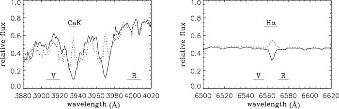
Figure 1. Spectrum of an active star (dotted line) and an inactive star (solid line). The solid lines under the letters indicate the wavelength regimes used to measure equivalent width (EW).
Download figure:
Standard image High-resolution image
Figure 2. (a) EWCaK vs. Teff. (b)  vs. Teff. Color is used to represent the ages of open clusters. (The data used to create this figure are available.)
Download figure:
Standard image High-resolution imageWe use a simple Monte Carlo simulation to obtain the error of EW. Detailed information can be found in Appendix A. For the Ca ii K line, the average error of EWCaK is about 0.1 Å when Teff > 5500 K. The average error of EWCaK is about 0.2 Å at Teff = 4500 K. For the Hα line, the average error of  is about 0.04 Å.
From Figure 2(a), it is clear that as Teff decreases, EWCaK first decreases and then increases. Figure 2(b) shows that as Teff decreases EWHα increases. As for the two panels, at high Teff range (Teff > 6500 K), member stars of different age populations mix. As Teff decreases, young member stars tend to have larger EW than old member stars, which conforms to our expectation. The scatter of EW increases as Teff decreases. Most member stars in our sample have Teff > 5500 K.
3.2. Excess EW
To measure  and
and  , basal lines are needed. The LAMOST official website provides the AFGK type (spectral type) star catalog. In this catalog, stars that satisfy 4000K < Teff < 7000 K, log g > 4.0, and S/N g > 30 (S/N r > 50), the same limitations as member stars, are selected. Further, only stars with −0.8 < [Fe/H] < 0.5 are selected because at poor [Fe/H] range ([Fe/H] ≤ −0.8) there is a negative correlation between EWCaK and [Fe/H]. We calculate their EWCaK and EWHα by the same method described in Section 3.1. Those stars with EW > 10 Å or EW < −10 Å are excluded. Figure 3 shows EWCaK versus Teff and EWHα versus Teff. This plot includes 1,563,898 stars for EWCaK and 1,581,197 stars for EWHα. Few stars are located at about 4570 K. This may be caused by a defect in the LAMOST pipeline at this Teff.

Figure 3. (a) EWCaK vs. Teff for stars in the LAMOST AFGK type star catalog. (b)  vs. Teff for stars in the same catalog. The scarcity of stars at about 4570 K may be caused by a defect in LAMOST pipeline at this Teff. The solid lines in the two panels are our basal lines. The left panel shows three basal lines corresponding to three different [Fe/H] ranges.
Download figure:
Standard image High-resolution imageBecause [Fe/H] has more effects on EWCaK than EWHα, we classify stars into three classes according to [Fe/H]: −0.8 < [Fe/H] < −0.2, −0.2 ≤ [Fe/H] < 0.1, and 0.1 ≤ [Fe/H] < 0.5 before determining the basal lines for EWCaK. For each class, we rebin the stars on Teff with a bin width of 50 K. In each bin, a 10% quantile is calculated in EWCaK. Then, five order polynomial is fitted to these quantiles as shown in the left panel of Figure 3. The solid lines are fitting curves. From the left panel we can see that the three basal lines corresponding to three different [Fe/H] ranges have some differences. When Teff > 6000 K, the basal line of the poor [Fe/H] range is above that of the rich [Fe/H] range. Generally speaking, poor [Fe/H] stars have larger EWCaK than rich [Fe/H] stars because for poor [Fe/H] stars' metallic lines are relatively shallow. Note that our EW is negative for an absorption line. For Hα, we directly rebin the stars on Teff with a bin width of 50 K without [Fe/H] classification and the basal line is obtained by the same method as above. The right panel of Figure 3 shows the basal line for EWHα. Then for member stars,  and
and  are obtained by using Equation (2). Stars whose
  are retained in our study.

3.3. Excess Fractional Luminosity
After obtaining EW', Equations (3) and (4) are used to calculate the excess fractional luminosity R'. In Equation (3), ATLAS9 model atmospheres8 are used to calculate χ of grid points. F(λ) is flux at the stellar surface. We choose λ = 3950.5 Å for Ca ii K and λ = 6560.0 Å for Hα. σ is the Stefan–Boltzmann constant. Turbulent velocity (vturb = 2.0 km s−1) and mixing length parameter (1/H = 1.25) are adopted for the model spectra. We calculate χ in terms of Teff, [Fe/H] and log g. Teff ranges from 4000 K to 7000 K in steps of 250 K. The values of log g range from 4.0 to 5.0 in steps of 0.5. [Fe/H] ranges from −2.5 to 0.5 in steps of 0.5 plus a value [Fe/H] = 0.2. Three dimensional linear interpolation is used to obtain the corresponding χ for each star. Finally, excess fractional luminosity R' is obtained by using Equation (4).


4. Results and Analysis
4.1. The Distribution of log R'
With the above procedures, log R' value for each member star is obtained. We perform a cross-match between our sample and the Simbad database,9
and exclude those stars labeled as "Flare*," "pMS*," "RSCVn," "SB*," "EB*WUMa," "EB*," "EB*Algol", and "EB*betLyr" by Simbad. Flare stars and binaries can affect CA level (Curtis 2017; Fang et al. 2018). In Appendix B, we simply discuss the impact of binaries. The result is shown in Figure 4. There are 1091 member stars in 82 open clusters with  values and 1118 member stars in 83 open clusters with
  values. Some open clusters are represented by only one or two stars. The Melotte 22 and NGC 2632 have over 100 member stars. From Figures 4(a) and (b), young member stars have similar log R' values as old member stars when Teff > 6500 K. As Teff decreases, young member stars tend to have larger log R' than old member stars, which conforms to our expectation. This phenomena is alike to Figure 2.

Figure 4. (a)  vs. Teff. (b)
  vs. Teff. (c)
  vs. [Fe/H]. (d)
  vs. [Fe/H]. The color has the same meaning as Figure 2. This plot includes 1091 member stars of 82 open clusters for Ca ii K and 1118 member stars of 83 open clusters for Hα, respectively.
Download figure:
Standard image High-resolution imageWe use a simple Monte Carlo simulation to obtain the error of log R'. Detailed information can be found in Appendix A. For the Ca ii K line,  has a large scatter when Teff > 6000 K (see Figure 10).
  is about 0.05 dex and 0.15 dex at 5500 K and 4500 K. For the Hα line, the distribution of
  has a large scatter from 0.0 to 0.5 dex at all Teff range (see Figure 10).
There are some member stars that should be noticed. In Figure 4(b), we can see that four member stars surrounded by a rectangle box have very high  values, which belong to the same open cluster: NGC 2112 (log t = 9.315). We check their spectra and find that they have very strong balmer emission lines. The open cluster is in the direction of the famous H ii region known as Barnard's loop (Haroon et al. 2017). We suspect that the high
  values of this cluster are caused by interstellar medium (ISM). In panels (a) and (b) of Figure 4, some member stars have very low values so that they will pull down the mean value of log R' within an open cluster and increase the scatter obviously. So we exclude those stars whose
  for the Ca ii K line and those stars whose
  for the Hα line in the following study.
Mamajek & Hillenbrand (2008) derived CA–age relation by using a traditional indicator  , which was derived from S-values in the Mount Wilson HK project (Vaughan et al. 1978; Noyes et al. 1984). We cross-match our results with Table 5 of Mamajek & Hillenbrand (2008). The comparison between our results and theirs is shown in Figure 5. The crossing match sample only includes three open clusters: Melotte 20, Melotte 22, and NGC 2682. From Figure 5, as
  or
or  decreases,
  also decreases. However, for those stars whose CA indices are low, our indices show a little larger scatter than theirs, which might be caused by different data-processing methods. For stars whose EW are close to the basal lines, their EW' are close to zero and the
  and
and  values discern more when taking the logarithm. In Appendix C, we list a table (Table 4) to illustrate it.
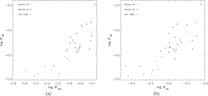
Figure 5. CA indices comparison for common stars between our sample and those from Mamajek & Hillenbrand (2008), which are member stars in three open clusters: Melotte 20, Melotte 22, and NGC 2682. The  and
and  are our CA indices. The
  are from Table 5 of Mamajek & Hillenbrand (2008).
Download figure:
Standard image High-resolution image4.2. log R' versus log t
4.2.1. log R' versus log t in Different Teff Ranges
The mean value of  (
( ) for each open cluster is calculated. Figure 6 plots this mean value versus the age of each cluster. The left-top corner gives the Teff range of member stars chosen to calculate mean value. Clusters that have only one star are not displayed in this plot. From Figure 6(a) we find that when stellar age log t < 8.5 (0.3 Gyr), the mean value of
  starts to decrease slowly as age increases. Then, after log t = 8.5, the mean value decreases rapidly until log t = 9.53 (3.4 Gyr). Soderblom et al. (1991) pointed out that the evolution of CA for a low-mass star may be going through three stages: a slow initial decline, a rapid decline at intermediate ages (∼1–2 Gyr), and a slow decline for old stars like the Sun. Although there are some differences on age ranges of each stage, our conclusion is consistent with that of Soderblom et al. (1991) for the two former stages. In our sample, the number of old open clusters (log t > 9.0) is small and the age is only extended to log t = 9.53, so it is hard to see whether there is a slow decline for old stars like the Sun. From Figure 6(b), the mean value of
  decreases from nearly log t = 6.76 (5.7 Myr) to log t = 9.53 (3.4 Gyr). Although it does not show the trend: a slow initial decline and then a rapid decline, we can see the same trend as Ca ii K if we divide the Teff range as done below.

Figure 6. Mean log R' vs. age log t among open clusters. Each triangle represents a cluster and the error bar indicates the standard deviation of the CA indices in each open cluster. Left-top corner gives the Teff range of stars chosen to calculate the mean values. Those clusters with only one member star are not displayed. Arrows are used to specify the location of some open clusters.
Download figure:
Standard image High-resolution imageFrom Figure 6, we can see some open clusters deviate from the location of our expectation or have a large error bar. In panel (a), three old open clusters (NGC 7789, NGC 2112, and NGC 2420) show a little larger mean values. Their average [Fe/H] are relatively poor compared to young open clusters. For example, NGC 2420 has average [Fe/H] equal to −0.278 ± 0.0462 (see Table 1). Poor [Fe/H] stars have relatively shallower metallic lines than rich [Fe/H] stars, leading to large  and
and  , which may be the reason of these larger mean values. Some open clusters have one or two member stars whose
  values are very low, so that they pull down the mean values, like Collinder 69 and Collinder 359. We see that NGC 1817 has a very large error bar. This cluster has five member stars and all stars are with Teff > 6500 K. Three of them have large
  values, the other two have low
  values. The difference between the two groups is about 1 dex. In panel (b), NGC 2112 has a very large mean value. The reason is discussed above.
The scatter of log R' within an open cluster is large. In addition to measurement error, there are many other physical factors contributed to the scatter. Within an open cluster, different member stars have different mass and rotation rates. Stellar mass and rotation rate can influence CA level (Noyes et al. 1984; Mamajek & Hillenbrand 2008). Stellar cycle modulations also change CA level (Baliunas et al. 1995; Lorenzo-Oliveira et al. 2018). Some stars in our sample may have flare or starspots, which affects CA level. Binaries and ISM can also influence CA level. Appendix B simply discusses the impact of binaries and ISM on log R'. In our sample, some stars may not belong to open clusters and they affect the mean values. Besides, our data-processing method also contributes to the scatter. For those stars whose EW are very close to the basal line, a small difference in EW between two stars can cause a large difference in log R' (see Table 4).
In order to decrease the influence of stellar mass on CA, we divide Teff into three equal bins and plot the mean log R' versus age log t again, as shown in Figure 7. In all Teff ranges, we can see the trend that as age increases the mean value decreases slowly or remains unchanged, and then decreases rapidly. The scatter is smaller at low Teff range than at high Teff range. That means log R' is more sensitive to stellar age at lower Teff, which is consistent with Figure 2 of Zhao et al. (2011). In their figure, the quantity log SHK used to indicate CA level discerned more from each other at redder color. The trend that CA shows a slow decline and then a rapid decline is more evident for cooler stars. This phenomena may be related to stellar inner structure. Those stars at low Teff range have thicker convective zone than those at high Teff range. So those stars at a low Teff range can maintain a strong surface magnetic field on a longer timescale than at a high Teff range (Fang et al. 2018; West et al. 2008).

Figure 7. Mean log R' vs. age (log t) among open clusters in different Teff ranges. Arrows are used to specify the location of some open clusters.
Download figure:
Standard image High-resolution imageThere are some open clusters that deviate from locations of expectation, or have a large error bar. Many of them are discussed above. In Figure 7(c), Melotte 25 has a low mean value and a large error bar. The reason is that this cluster has only three member stars at 6000 K < Teff < 7000 K, of which one member star has a low  value (
 ), pulling down the mean value. In Figure 7(d), Alessi 20 has a larger mean value. With 4000 K < Teff < 5000 K, this open cluster has only two member stars, whose [Fe/H] are poorer compared to the other member stars. One of these two stars shows very strong Hα emission line. Maybe these two stars are not member stars of the cluster. Roslund 6 has only two member stars with 4000 K < Teff < 5000 K. The
  of these two stars are very large. One is 15.13 Å, the other is 3.90 Å. Their spectra show very strong H α emission line. This is not just Hα, there are other emission lines in these two spectra such as: Hβ, Ca ii HK, N ii, and so on. Maybe the two stars are in a special term. For example, they have large spots on stellar surface.
4.2.2. log R' versus log t in a Narrow [Fe/H] Range
[Fe/H] has more of an effect on  than
than  (Rocha-Pinto & Maciel 1998; Rocha-Pinto et al. 2000; Lorenzo-Oliveira et al. 2016). Maybe there is a negative correlation between
  and [Fe/H]. We narrow the [Fe/H] range to −0.2 < [Fe/H] < 0.2 and plot the mean log R' versus age log t again. The sample is split on a star-by-star basis. Figure 8 shows log R' versus log t with 4000 K < Teff < 7000 K and −0.2 < [Fe/H] < 0.2. By comparing Figures 8 and 6, we find that there is no obvious difference. Figures 9(a) and (c) show log R' versus log t with 4000 K < Teff < 5500 K and without [Fe/H] limit. Figures 9(b) and (d) show log R' versus log t with 4000 K < Teff < 5500 K and −0.2 < [Fe/H] < 0.2. By comparison, no obvious difference is formed. We also see no large difference of log R' versus log t relation when narrowing the [Fe/H] range to −0.1 < [Fe/H] < 0.1.
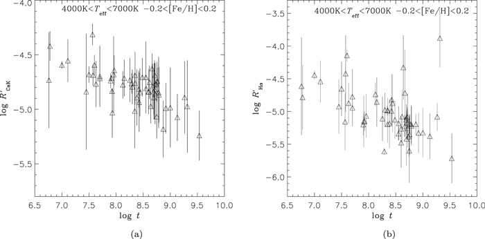
Figure 8. Mean log R' vs. age (log t) among open clusters with 4000 K < Teff < 7000 K and −0.2< [Fe/H] < 0.2.
Download figure:
Standard image High-resolution image
Figure 9. Mean log R' vs. age (log t) with 4000 K < Teff < 5500 K in two [Fe/H] ranges. Quadratic function is used to fit these data points. Relationship is listed in the left-bottom corner. For Hα, two stars of Alessi 20 and two stars of Roslund 6 mentioned in Section 4.2.1 are removed.
Download figure:
Standard image High-resolution image4.3. Fitting between log R' and log t at low Teff Range
Quadratic function is used to fit data points with 4000 K < Teff < 5500 K in two [Fe/H] ranges. Figure 9 shows fitting curves and relationships. For Hα, two stars of Alessi 20 and two stars of Roslund 6 mentioned in Section 4.2.1 are removed. The relationships are also listed in Equations (5)–(8). Age for field stars can be approximately estimated by solving these quadratic equations. Via Monte Carlo simulation, a distribution of log t can be obtained with a log R' value and its error. For Equations (5) and (6), we calculate two distribution of log t at two  values (
 ). The error of
  is set to 0.15 dex. The errors of log t are about 0.40 dex, 0.28 dex at log t = 8.75, 9.44 corresponding to
  . The error of log t at log t = 9.44 is smaller than at log t = 8.75. This is because the fitting curve gets steeper when log t increases and
  is projected to a smaller range of log t. For Equations (7) and (8), the errors of log t are about 0.40 dex, 0.28 dex at log t = 8.60, 9.40 corresponding to log
  . The error of
  is set to 0.20 dex.
Equations (5) and (7) are used to estimate ages of corresponding clusters whose log t > 8.00. The results and relative error are shown in Table 3. The accuracy of Equation (5) is about 40%, while the accuracy of Equation (7) is about 60%. The ages of NGC 1647 and Ascc 10 cannot be estimated by Equation (5) because the two clusters have very large  mean values that exceed the maximum value of Equation (5).
Table 3. Estimated Ages of Corresponding Open Clusters Whose log t > 8.00
| Name | t | Equation (5) | Relative Error | Equation (7) | Relative Error |
|---|---|---|---|---|---|
| (Myr) | (Myr) | (Myr) | |||
| Melotte_22 | 141 | 176 | 25% | 147 | 4% |
| NGC_2168 | 180 | 58 | 68% | ||
| NGC_1647 | 200 | 93 | 53% | ||
| NGC_1039 | 242 | 732 | 203% | 380 | 57% |
| Stock_10 | 263 | 405 | 54% | 237 | 10% |
| ASCC_23 | 305 | 249 | 19% | 582 | 91% |
| NGC_1342 | 398 | 424 | 6% | ||
| NGC_1750 | 414 | 696 | 68% | 157 | 62% |
| Roslund_6 | 468 | 292 | 38% | 80 | 83% |
| NGC_1662 | 495 | 580 | 17% | 580 | 17% |
| ASCC_41 | 501 | 661 | 32% | 623 | 24% |
| Collinder_350 | 513 | 676 | 32% | ||
| ASCC_10 | 521 | 283 | 46% | ||
| NGC_2281 | 610 | 526 | 14% | 566 | 7% |
| IC_4756 | 617 | 766 | 24% | 1088 | 76% |
| Melotte_25 | 741 | 1788 | 141% | 1950 | 163% |
| NGC_2632 | 832 | 1169 | 41% | 1150 | 38% |
| NGC_752 | 1349 | 1258 | 7% | 1495 | 11% |
| NGC_2682 | 3428 | 2918 | 15% | 2403 | 30% |
Note.The first column is the names of open clusters. The second column is the ages (t) of clusters from references. The third and fourth columns are the estimated ages from Equation (5) and its relative error. The fifth and sixth columns are the estimated ages from Equation (7) and its relative error.
Download table as: ASCIITypeset image
Equations (5) and (7) are also used to estimate ages of open clusters whose ages are not found in literatures. However, only the open cluster RSG 1 is available to estimate age. The cluster has log t = 8.69 estimated by Equation (5) and log t = 8.52 estimated by Equation (7). In a following paper, we will use Equations (5)–(8) to roughly estimate ages of field stars.


5. Conclusion and Outlook
In this paper, we investigate the CA–age relationship by using the largest sample of open clusters in the LAMOST survey. Fang's method (Fang et al. 2018) is used to calculate excess fractional luminosity  ,
,  of every member star that can be used to indicate CA level. In this method, we use a 10% quantile in EW to obtain the basal lines. EW' can be obtained after subtracting EWbasal. Then R' can be obtained via
  , of which χ is the ratio of the surface continuum flux near the line to the stellar surface bolometric flux from model spectra.
For each open cluster, the average  ,
,  can be calculated. For Ca ii K, 1091 member stars of 82 open clusters have
  measurements. For Hα, 1118 member stars of 83 open clusters have
  measurements. Then the relationship between the average log R' and the age can be studied in different Teff ranges and [Fe/H] ranges. We find that CA starts to decrease slowly from log t = 6.70 to log t = 8.50, then decreases rapidly until log t = 9.53, which is consistent with the point of Soderblom et al. (1991). The trend is more evident for cooler stars. This phenomena may be related to stellar inner structure. Compared to stars at high Teff, stars at low Teff have thicker convective zone, such that they can maintain a strong surface magnetic field at longer timescale. We narrow the [Fe/H] range to −0.2 < [Fe/H] < 0.2 and find that there is no obvious difference. Finally, we construct quadratic functions between log R' and log t with 4000 K < Teff < 5500 K, which can be used to roughly estimate ages of field stars with accuracy about 40% for
  and 60% for
  .
.
The LAMOST telescope has obtained about 9 million spectra. The relations shown in Equations (5)–(8) suggest that  can be used to roughly estimate stellar ages for dwarfs. With reliable stellar ages, the evolution of the thin disk can be investigated. For example, we can study the spatial age distribution and relations between the stellar age and velocity. Older open clusters are needed to extend the CA–age relation. Medium resolution spectra (R ∼ 8000) being obtained with the ongoing LAMOST survey may improve the CA–age relation in the near future.
This study is supported by the National Natural Science Foundation of China under grants Nos. 11988101, 11625313, 11890694, 11573035,11973048, 11927804, and the National Key R&D program of China No. 2019YFA0405502. Support from the US National Science Foundation (AST-1358787) to Embry-Riddle Aeronautical University is acknowledged. Guoshoujing Telescope (the Large Sky Area Multi-Object Fiber Spectroscopic Telescope LAMOST) is a National Major Scientific Project built by the Chinese Academy of Sciences. Funding for the project has been provided by the National Development and Reform Commission. LAMOST is operated and managed by the National Astronomical Observatories, Chinese Academy of Sciences.
Appendix A: Measurement Error of EW and log R'
Monte Carlo simulation is used to obtain the error of EW. For a spectrum, flux at every data point has a inverse variance. So the random flux can be produced following a Gaussian distribution of μ (flux at a data point) and σ (inverse variance). In our simulation, we produce 1000 simulated spectra and calculate their EW. The standard deviation of EW is used as the error of EW. Figures 10(a) and (b) plot σ (EW) versus Teff. From Figure 10(a), the error of EWCaK increases slightly as Teff decreases. The average error of EWCaK is about 0.1 Å when Teff > 5500 K and about 0.2 Å at Teff = 4500 K. From Figure 10(b), we see that the bottom boundary of distribution of  increases slightly when Teff decreases from 5500 K. The average error of EWHα is about 0.04 Å.
The error of log R' is also estimated by using Monte Carlo simulation again. Only four factors are considered: the EW and stellar atmospheric parameters including Teff, [Fe/H], and log g. Errors of Teff, [Fe/H], and log g are set to 110 K, 0.12 dex, and 0.11 dex, respectively. Figures 10(c) and (d) show  versus Teff. From Figure 10(c), we see that when
  K,
K,  shows a large scatter. The large scatter is mainly due to small
  , which means EWCaK are close to the basal line. If a star has EWCaK close to the basal line, its
  is close to zero. A small difference in EWCaK can cause a large difference in
  when taking logarithm of R' (
 ). When
  K,
K,  shows a relatively tight distribution. The errors are about 0.05 dex and 0.15 dex at 5500 and 4500 K, respectively. There is no large scatter at this Teff range because as Teff decreases the distribution of EWCaK shows a large scatter (see Figure 2) and many stars have relatively large
  . From Figure 10(d), we see that at all Teff range
  show a very large scatter from 0.0–0.5 dex. The reason is same as above. However, for the Hα, many member stars have
  close to the basal line not only at high Teff range but also at low Teff range.
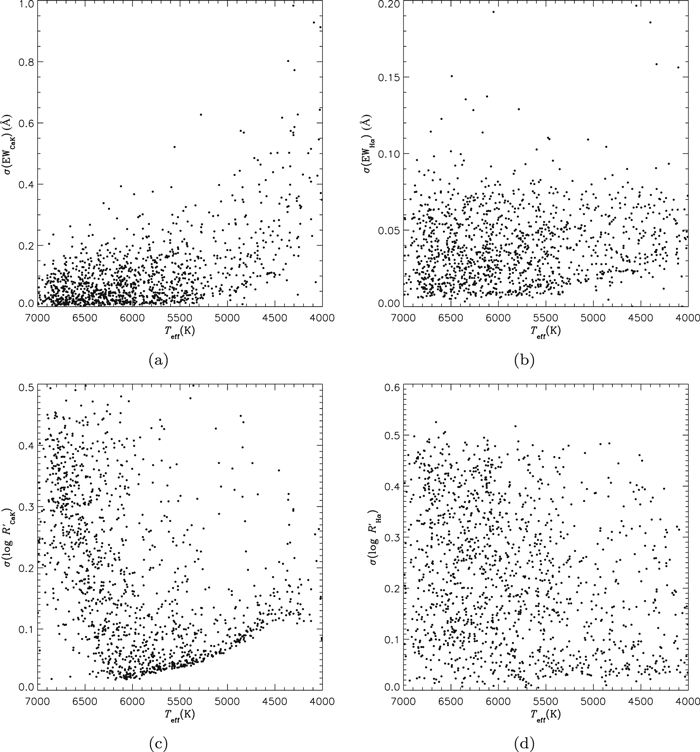
Figure 10. (a) σ(EWCaK) vs. Teff. (b)  vs. Teff. (c)
  vs. Teff. (d)
  vs. Teff.
Download figure:
Standard image High-resolution imageAppendix B: The Impact of Binaries and Interstellar Medium on log R'
The interaction of two stars can affect CA level. The member stars list provided by Cantat-Gaudin et al. (2018) include Gaia color (GBP–GRP) and visual magnitude (Gmag). According to this information, we can plot the color–magnitude diagram (CMD) of each open cluster. On the CMD, some member stars lie above the single main sequence and many of them are binaries. We try to check the change of the mean value and scatter of log R' by discarding these stars. For example, after discarding these stars of NGC 2632, the mean value and standard error of  changes from −5.04 ± 0.184 to −5.05 ± 0.184 with 4000 K < Teff < 5500 K. The same value of
  changes from −5.16 ± 0.185 to −5.18 ± 0.178 with 4000 K < Teff < 5500 K. Note that we do not consider the labels provided by simbad. The change of the mean values is very small.
The ISM imprints absorption lines in the vicinity of the Ca ii H and K line cores, which negatively biases CA indices (Pace & Pasquini 2004; Curtis 2017). Our spectra are low resolution spectra (R ∼1800 at 5500 Å) and they are not very likely to show evident ISM absorption lines at the wavelength of the Ca ii H and K line. Hα line is less affected by ISM. So we can find some open clusters which are coeval but separated by a large distance. Then we plot the distributions of  versus Teff and
  versus Teff. If ISM affect our results, at a similar range of Teff, the
  values of nearby cluster are supposed to be higher than that of distant cluster, but the
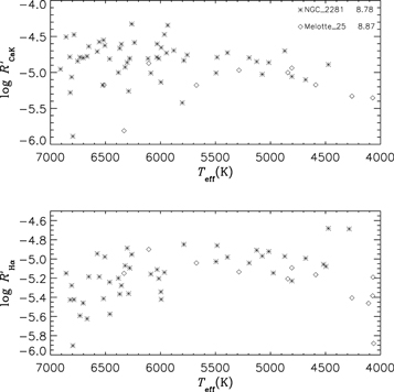
  values should keep consistent. However, in our sample, the number of member stars for some open clusters are small. Besides, many open clusters have most member stars with Teff > 6000 K. When Teff > 6000 K, log R' values of member stars of different ages can mix. Fortunately, we find two open clusters: NGC 2281 and Melotte 25 (Hyades). NGC 2281 has log t = 8.78 (Kharchenko et al. 2013) and d = 519 pc (Cantat-Gaudin et al. 2018). d is the distance to the Sun. Melotte 25 has log t = 8.87 (Gossage et al. 2018) and d = 48 pc (Röser et al. 2019). There is more than 100 Myr age difference between the two clusters. The distributions of log R' versus Teff are shown in Figure 11. When Teff < 6000 K, NGC 2281 has slightly larger
  and
and  values than that of Melotte 25 at a similar range of Teff, which suggests that the impact of ISM is smaller compared to the decrease in CA over time.
Figure 11. Top panel is  vs. Teff. Bottom panel is
  vs. Teff. The asterisk represents for NGC 2281 while the diamond represents for Melotte 25.
Download figure:
Standard image High-resolution image
Appendix C: An Illustration of Logarithm Effect
During data processing, the EW of some member stars are close to the basal lines. For those stars, a small difference in EW can cause a large difference in log R'. This is because EW close to the basal line leads to EW' close to zero and R' close to zero ( ), then R' is projected to a large range when taking logarithm. We list some examples in Table 4 to illustrate it.
Table 4. Some Examples to Illustrate Logarithm Effect
| Teff(K) | EWCaK(Å) |

|
 (Å) (Å) |

|
|---|---|---|---|---|
| 6500 | −4.50 | −4.92 | −2.50 | −5.75 |
| 6500 | −4.00 | −4.46 | −2.00 | −4.77 |
| 6500 | −3.50 | −4.24 | −1.50 | −4.49 |
| 5500 | −5.00 | −5.42 | −1.70 | −5.74 |
| 5500 | −4.50 | −4.83 | −1.20 | −4.72 |
| 5500 | −4.00 | −4.59 | −0.70 | −4.44 |
| 4500 | −4.50 | −5.59 | −0.70 | −5.40 |
| 4500 | −4.00 | −5.25 | −0.20 | −4.71 |
| 4500 | −3.50 | −5.06 | 0.30 | −4.46 |
Note. Note that [Fe/H] and log g are set to 0.0 and 4.2.
Download table as: ASCIITypeset image
Footnotes
- 7
- 8
- 9