


Abstract
The Chromospheric Lyman-Alpha Spectro-Polarimeter (CLASP) sounding rocket experiment, launched in 2015 September, observed the hydrogen Lyα line (121.6 nm) in an unprecedented high temporal cadence of 0.3 s. CLASP performed sit-and-stare observations of the quiet Sun near the limb for 5 minutes with a slit perpendicular to the limb and successfully captured an off-limb spicule evolving along the slit. The Lyα line is well suited for investigating how spicules affect the corona because it is sensitive to higher temperatures than other chromospheric lines, owing to its large optical thickness. We found high-frequency oscillations of the Doppler velocity with periods of 20–50 s and low-frequency oscillation of periods of ∼240 s on the spicule. From a wavelet analysis of the time sequence data of the Doppler velocity, in the early phase of the spicule evolution, we found that waves with a period of ∼30 s and a velocity amplitude of 2–3 km s−1 propagated upward along the spicule with a phase velocity of ∼470 km s−1. In contrast, in the later phase, possible downward and standing waves with smaller velocity amplitudes were also observed. The high-frequency waves observed in the early phase of the spicule evolution would be related with the dynamics and the formation of the spicules. Our analysis enabled us to identify the upward, downward, and standing waves along the spicule and to obtain the velocity amplitude of each wave directly from the Doppler velocity for the first time. We evaluated the energy flux by the upward-propagating waves along the spicule, and discussed the impact to the coronal heating.
Export citation and abstract BibTeX RIS
1. Introduction
To maintain the solar corona at a temperature of around 106 K, magnetic energy needs to be transported from the photosphere. The chromosphere, which is the middle layer between the photosphere and the corona, is thought to play an important role to transfer the energy for the coronal heating. In the chromosphere, vertically elongated structures called spicules are observed everywhere and it is of great interest to understand how these ubiquitous phenomena are relevant to the coronal heating.
In previous studies, two types of oscillation period (shorter than 2 minutes and longer than 2 minutes) had been observed in spicules (reviewed by Zaqarashvili & Erdélyi 2009). Long-period oscillations with periods of 2–8 minutes were found from the apparent motions of spicules using imaging observations (De Pontieu et al. 2007; McIntosh et al. 2011). These oscillations are considered to be magnetohydrodynamic waves, which can transport sufficient energy to heat the quiet corona because of the large velocity amplitude. However, because the wavelengths of these long-period oscillations are longer than the typical spicule height (5–20 Mm; Alissandrakis et al. 2005; Teriaca et al. 2006; De Pontieu et al. 2007; Pasachoff et al. 2009), it remains uncertain whether such oscillations propagate along spicules as a wave or not.
The wave propagation of short-period lateral oscillations (shorter than 2 minutes period) had been observed (He et al. 2009; Okamoto & De Pontieu 2011; Srivastava et al. 2017) thanks to the high temporal (shorter than 10 s) and high spatial (smaller than 0 2) resolution of the Solar Optical Telescope (SOT) onboard the Hinode satellite (Kosugi et al. 2007), and ground-based observatories, such as the Swedish 1 m Solar Telescope/CRisp Imaging SpectroPolarimeter (SST/CRISP; Scharmer et al. 2003, 2008). The reason why they were able to detect wave propagations is because the wavelengths of these oscillations are shorter than the typical spicule height. Particularly, Okamoto & De Pontieu (2011) found not only upward but also downward propagation and standing waves for the first time by using the automatic spicule axis detection method. They concluded that high-frequency waves are not sufficient for coronal heating because most high-frequency waves are reflected at the transition region and the velocity amplitudes of the waves are so small.
To solve the coronal heating problem, the transported energy to the corona needs to be evaluated quantitatively with as few assumptions as possible. The velocity amplitude is an important parameter to evaluate the transported energy flux. Spectroscopic observation is a direct way to derive the velocity amplitude. In this study, we analyzed the Lyα (121.6 nm) line profile of an off-limb spicule observed by Chromospheric Lyman-Alpha Spectro-Polarimeter (CLASP; Kano et al. 2012; Kobayashi et al. 2012; Narukage et al. 2015) and evaluated the Doppler velocity amplitude.
CLASP is a sounding rocket experiment that obtained Lyα spectro-polarimetric data with a 0.3 s temporal cadence for the polarization modulation (Kano et al. 2017; Ishikawa et al. 2017a). If we do not use the Stokes spectra of Q/I and U/I, we can utilize such an unprecedentedly high temporal cadence data to study the dynamics in the upper chromosphere and the transition region. The Lyα line is well suited to investigate how spicules affect the corona because it is sensitive to higher temperatures than other chromospheric lines (e.g., Ca ii H, Mg ii h, and k) because of the large optical thickness. Alissandrakis et al. (2005) reported that Lyα spicules exhibit a height of approximately 25'' (18 Mm; 1'' ≈730 km on the Sun) from the limb using the Transition Region and Coronal Explorer (Handy et al. 1999), which are taller than the spicules observed in the visible wavelengths (e.g., 4–12 Mm in the Hα line by Pasachoff et al. 2009, and 5–10 Mm in the Ca ii H line by De Pontieu et al. 2007). Teriaca et al. (2006) found intensity fluctuations of 3 and 5 minutes periods in off-limb spicules with a temporal cadence of 7.5 s using the Solar Ultraviolet Measurements of Emitted Radiation (Wilhelm et al. 1995) but they did not discuss a shorter period than 2 minutes. In this study, we focus on the wave propagation along a spicule that can be observed spectroscopically by CLASP with an unprecedentedly high temporal cadence of 0.3 s.
2. Observation and Analysis
CLASP observed the quiet-Sun region near the limb for 277.2 s from 17:03 UT to 17:08 UT on 2015 September 3. The CLASP Spectro-Polarimeter (SP) acquired Lyα spectroscopic data with a 0.3 s temporal cadence, while CLASP Slit-Jaw (SJ) acquired Lyα filter images with a 0.6 s temporal cadence. The SP slit with a width of 145 was located 26'' outside of the photospheric solar limb and perpendicular to the southwest limb inclined at −37° with respect to the solar north. During the observation, one spicule was located along the slit (Figure 1) and evolved beyond the edge of the slit. We focus on this spicule in this study. Because the duration of the CLASP observation may be shorter than the typical spicule lifetime (2–12 minutes; Tsiropoula et al. 2012), we check the behavior of the spicule before and after the CLASP observation by using the Solar Dynamics Observatory/Atmospheric Imaging Assembly (SDO/AIA; Lemen et al. 2012; Pesnell et al. 2012) 30.4 nm (He ii line) filter image. The structural similarity between the SJ Lyα filter and AIA 30.4 nm filter images were reported by Kubo et al. (2016) and Ishikawa et al. (2017b) for the on-disk features. We used the SDO/Helioseismic and Magnetic Imager (HMI; Schou et al. 2012) continuum images to check the spicule height from the photospheric limb. Note that the spatial and spectral resolutions of CLASP SP are ∼3'' and ∼0.010 nm, respectively (Giono et al. 2016). From the temporal resolution of SP, the Nyquist frequency is about 1.6 Hz. However for the polarization observation, the rotation period of the wave plate is 4.8 s, and the image wobbled by the rotation. Considering its influence, we focused only on the oscillation longer than 4.8 s.
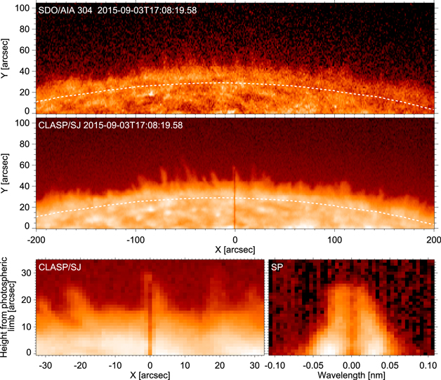
Figure 1. (Top) AIA 30.4 nm filter image. (Middle) Same field of view of Lyα filter image taken with CLASP/SJ as the top panel of AIA image. A vertical black line around X = 0'' is the slit. Dotted lines in the top and middle panels show the position of the photospheric limb determined by the SDO/HMI continuum intensity. (Bottom left) Enlarged image of SJ filter image around the slit position. (Bottom right) Spectral data of the Lyα line at the slit position as a function of wavelength from the line center (121.6 nm). The vertical axis of the bottom two panels indicates height from the photospheric limb. The height = 0 and X = 0 in the bottom left panel corresponds solar-X = 572'' and solar-Y = −762'' on the heliocentric coordinate. These snapshots correspond to the time of the last CLASP observational image.
Download figure:
Standard image High-resolution imageAs shown in Figures 2 and 3, the profile of the Lyα in the spicule shows central reversal as commonly observed in the quiet-Sun regions (Tian et al. 2009). The presence of the central reversal in the off-limb spicule indicates the large opacity. The central 2–3 pixels in the self-reversal are also affected by the geo-coronal absorption, which came from the atmosphere of the Earth (Gouttebroze et al. 1978). Therefore, we applied the bisector method to derive the Doppler velocity from the wing of the Lyα line. As shown in Figure 3, in this method the Doppler velocity was determined from the bisector position between the red and blue sides of the emission line at a threshold. Because the continuum intensity level is 10%–20% of the maximum intensity in the data, we chose 30% of the maximum intensity as the threshold. We also calculated the Doppler velocity with a different threshold (40% and 50%); however, the differences of Doppler velocity between the results with 30%, 40%, and 50% thresholds were less than 2 km s−1.

Figure 2. The Lyα line profile of the spicule at each height from the photospheric limb. The height step corresponds to the SP spatial plate scale (1.11 arcsec pixel−1). The horizontal axis is time, and the vertical axis in each box indicates wavelength as shown on the left side. The origin of the time corresponds to the start of the limb observation.
Download figure:
Standard image High-resolution image
Figure 3. Examples of Lyα line profile at time = 78 s (top) and 180 s (bottom) at height = 167 from the photospheric limb. Three asterisk symbols indicate the bisector at three different thresholds (30%, 40%, and 50%).
Download figure:
Standard image High-resolution imageThe error in the Doppler velocity mainly comes from a photon noise. So, we estimated the error as the difference of the Doppler velocity from close threshold levels; 30%, 35%, and 40%. We made an ensemble of thus derived errors of the Doppler velocity for the whole data set and derived the standard deviation of ±0.6 km s−1 as the error in the Doppler velocity.
3. Results
3.1. Temporal Evolution of Spicule
The time-slice of the spicule in the AIA 30.4 nm filter image (left panel of Figure 4) shows that this spicule exhibits a lifetime of roughly 13 minutes (from 0 to 800 s time range). The white box in Figure 4 indicates the region and duration observed by CLASP and demonstrates that CLASP observed the clear rising motion over the time range of 0–400 s with 30 km s−1. By comparing the left panel of Figure 4 and the right top panel of Figure 4 or top and middle panels of Figure 1, one can see that the AIA 30.4 nm image and the CLASP Lyα image represent the similar appearances of the spicules. However, it is also clear that the AIA 30.4 nm image is very noisy and hard to discuss the detail of the spicule dynamics solely with the AIA 30.4 nm image. As shown in the bottom left panel of Figure 1, the height of the spicule is about 30'', which corresponds to approximately 20 Mm from the photospheric limb. We confirmed that the spicule that we focus on is sufficiently high enough to investigate the wave propagation along it.

Figure 4. (Left) Time-slice image of the spicule observed by the AIA 30.4 nm filter. The white box indicates the height–time region corresponding to the SP spicule data (i.e., right panels.) (Top right) Height–time map of the spicule in the SP intensity. (Bottom right) Height–time map of the Doppler velocity. The top-left part of this panel colored by black is a masked area due to low intensity. The white arrows indicate the short-period velocity oscillations. In each panel, the vertical axis is the height from the photospheric limb. The white dotted lines and values in the left and top right panels indicate the spicule rising velocity. The black dotted lines and values shown in the bottom right panel correspond to the reference gradients of the phase velocity.
Download figure:
Standard image High-resolution image3.2. Temporal Variation of Doppler Velocity
Figure 2 shows the temporal variation of the Lyα spectral line at different heights of the spicule from the photospheric limb. The center of the Lyα line (central reversed part) did not shift as much. However, the wing clearly shifted in the wavelength direction.
The lower right panel of Figure 4 shows the height–time map of the Doppler velocity of the spicule derived by the bisector method. The low-intensity area masked by the black color is not used in this analysis. At first, we found a long-period oscillation in this map, i.e., the blueshift (−20 km s−1) until 120 s, followed by the redshift (20 km s−1) until about 240 s, and then finally the blueshift again. The period of this oscillation is about 240 s. We also found a short-period oscillation with a period of about 30 s in the time range of 0–100 s, as indicated by white arrows. Its velocity amplitude is about 5 km s−1. The ridges with large velocity amplitudes (i.e., dark blue regions) incline with time as the height increases. This indicates that these oscillations propagate in the upward direction; that is, we found the upward-propagating wave. We estimated the propagation velocity of the wave to be 200–500 km s−1 from the tilt of the ridges in short-period oscillations. The velocity amplitudes increase with spicule height. On the other hand, the propagation of the long-period oscillation is not clear from this observation, because the observed spicule height (∼20 Mm) is shorter than the wavelength of the long-period oscillation of 120 Mm, where we assumed a phase velocity of 500 km s−1 and an oscillation period of 240 s. In the following section, we highlight the short-period oscillations.
3.3. Wavelet Analysis
To investigate the propagation properties of the short-period waves in detail, we applied wavelet analysis to the Doppler velocity time-series data at each height shown in the bottom right panel of Figure 4. Figure 5 shows the normalized wavelet power spectra at each height along the spicule. In this analysis, we used the wavelet analysis program by Torrence & Compo (1998). Generally, time resolution and frequency resolution are different depending on the type of mother wavelet function. In this analysis, the Morlet wavelet function, which has a good frequency resolution but poor temporal resolution, was taken as the mother function. We defined the time-dependent confidence level (so-called "global" wavelet confidence level) as a probability calculated using Monte-Carlo simulation and the background noise model as a power law plus white noise model (Auchère et al. 2016). In Figure 5, the wavelet power is normalized by the background noise. The area encircled by a thick black line indicates a confidence level larger than 99%. This level means that such an event is expected to occur in only one case in 100 random data sets. We also checked the results of the 90% confidence level; however, the results were not significantly different from the 99% results. In the time range of 0–100 s in Figures 5(a)–(c), the oscillations of frequency 33–50 mHz (20–30 s; hereafter called the 30 s wave) are prominent; their confidence levels exceed 99%. In Figures 5(i) and (j), the oscillations of 19–27 mHz (37–53 s; hereafter called the 50 s wave) exist with a relatively longer duration than that of the 30 s wave. The wavelet power of the 30 s wave is strong in the higher part of the spicule, while the wavelet power of the 50 s wave is strong in the lower part of the spicule. We also used the Paul mother function, which has good temporal resolution but poor frequency resolution, we got similar results—around 30 s period oscillations in the early phase on the upper part of the spicule and around 50 s period oscillations in the lower part of the spicule existing long duration. We do not see prominent powers exceeding the 99% confidence level in the period range from 4.8 to 20 s. The results of wavelet analysis with a different thresholds of the bisector analysis are given in the Appendix (Figure 7).
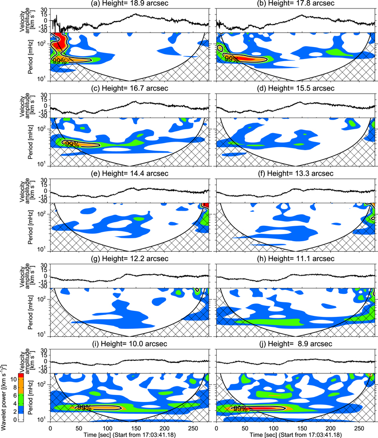
Figure 5. The results of wavelet analysis and curves of Doppler velocity. Each panel indicates the result at a different height from the photospheric limb. Cross-hatched areas correspond to the cone-of-influence, which is affected by the edge (discontinuity at the start timing and end timing). Areas covered by a thick black line correspond to the 99% confidence level.
Download figure:
Standard image High-resolution imageTo extract the wavelet power of the 30 s wave and the 50 s wave, we applied a box-type frequency filter of 33–50 mHz and 19–27 mHz frequency range, respectively, and then applied the inverse wavelet (Figure 6). In this figure, the regions covered with gray color correspond to the height and time ranges where there is no 99% significance wavelet power. Only a few areas are reliable in terms of velocity amplitude and phase velocity based on the wavelet analysis with confidence-level calculation.
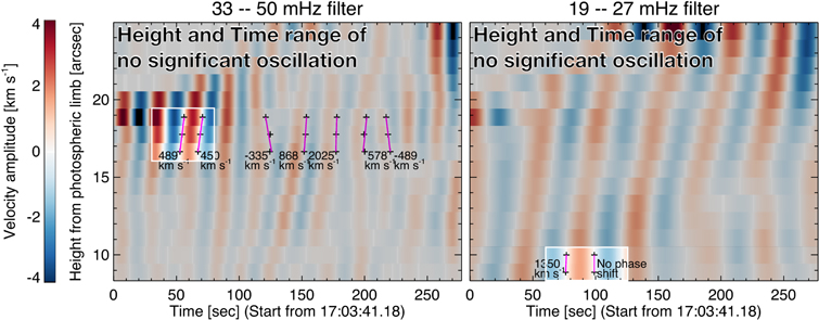
Figure 6. The result from the 30 s wave filter (33–50 mHz; left) and 50 s wave filter (19–27 mHz; right). The gray masked area corresponds to the height or timing at which there is no 99% significance wavelet power in each frequency range. The purple lines and values indicate the phase velocity calculated by linear fitting of zero-crossing timings.
Download figure:
Standard image High-resolution imageFrom the results of the 30 s wave filter (left panel), the waves with a velocity amplitude of ∼3 km s−1 propagate upward with a phase velocity of ∼470 km s−1 on average in the time range of 30–80 s. In addition, the velocity amplitude of the wave gets larger with height (from ±2 km s−1 at 167 to ±3 km s−1 at 189). Meanwhile, after 100 s to the end of the observation, the velocity amplitude of the 30 s wave became significantly small (less than 2 km s−1) and the confidence level became lower than 99%. Therefore, it is true the phase velocity is not reliable in this latter time range, but both upward and downward propagations might exist here as well as the standing waves, which do not exhibit a clear phase shift along the height direction (i.e., higher than 1000 km s−1).
From the results of the 50 s wave filter (right panel), standing waves with no clear phase shift were observed with the 99% confidence. The velocity amplitude of these waves is also prominent in the early phase, but small (∼2 km s−1) compared with the 30 s waves.
4. Discussion
In this study, short-period (20–50 s) waves with a small velocity amplitude of 2–3 km s−1 were found, as well as long-period (∼240 s) oscillation with a large velocity amplitude of ∼20 km s−1. The upward-propagating wave was also found in the short-period waves, especially around the period of 30 s, although it is not clear whether the latter long-period waves propagate along the spicule or not. Previous studies (De Pontieu et al. 2007; He et al. 2009; McIntosh et al. 2011; Okamoto & De Pontieu 2011; Srivastava et al. 2017) have reported these oscillation components separately; however, this is the first time that both oscillation components were detected simultaneously. This is because the velocity amplitudes of a long spicule are successfully obtained directly from the spectroscopic data in the Lyα line.
In this section, we will discuss the physical properties of the long-period oscillation and the short-period waves focusing on how they are formed and how they affect the corona.
4.1. Long-period Oscillations
De Pontieu et al. (2007) reported oscillations with a period of 100–500 s and a velocity amplitude of 10–25 km s−1 in spicules, from the comparison between the observation of the lateral motion of spicules and the Monte-Carlo simulation. Tomczyk et al. (2007) and Tomczyk & McIntosh (2009) found long-period (5 minutes) propagating waves in the corona using the Coronal Multi-channel Polarimeter (CoMP) instrument. However, their velocity amplitude was measured to be less than 1 km s−1 and much smaller than what was inferred from the chromospheric observations by De Pontieu et al. (2007). Tomczyk et al. (2007) speculated that the velocity amplitudes are suppressed due to the superpositions of the structures along the line-of-sight direction in CoMP observations, resulting in the large discrepancy in the velocity amplitudes between the chromosphere and the corona. In fact, nonthermal velocity derived from the CoMP line width is 30 km s−1 and is comparable to the velocity amplitude that was found in our observation, where the superposition along the line of sight is unlikely. Therefore, there is a possibility that the long-period oscillation in our observation is a chromospheric counterpart of the propagating waves in the corona.
The period of the long-period oscillation is on the order of the photospheric convection timescale, approximately 3–5 minutes (Matsumoto & Kitai 2010). One explanation is that the convective motion would oscillate the magnetic flux tube; then, the line-of-sight component of the oscillation is observed as the Doppler motion.
4.2. Short-period Waves
Okamoto & De Pontieu (2011) reported oscillation periods peaking near 40 s from statistical analysis using the Hinode/SOT filtergraphic data. They derived a median velocity amplitude of 7 km s−1 using the apparent transverse oscillation amplitude and period of the spicules, assuming the oscillation follows a sinusoidal pattern. Our observed period derived from Doppler motion (20–50 s) is almost consistent with their observation. Our observed velocity amplitude is slightly smaller than their reported value. One of explanations for our smaller velocity amplitude would be the difference in spatial resolution between CLASP/SP (∼3''; Giono et al. 2016) and Hinode/SOT (∼02; Suematsu et al. 2008). The lower spatial resolution causes the smearing and underestimation of the velocity amplitudes.
The phase velocity (∼470 km s−1) of the 30 s wave is roughly consistent with the Alfvén velocity in the upper chromosphere where we assumed a magnetic field strength of 10 G (Trujillo Bueno et al. 2005) and a spicule density of 6 × 10⁻¹⁵ g cm−3 (at 18 Mm height from the photosphere; Beckers 1968). We derived the fast phase velocity (i.e., higher than 1000 km s−1) in this study, and recognized them as a standing wave by considering the observed phase difference. Since 1000 km s−1 is much higher than the Alfvén velocity in the chromosphere, such recognition looks reasonable from the viewpoint of the physical property in the chromosphere.
Upward-propagating waves with a large velocity amplitude were observed, especially in the initial phase of the spicule evolution. This result implies that the source of these waves would be related to the formation of the spicule. Spicule formation by waves has been reported in a number of previous studies by numerical simulation. Kudoh & Shibata (1999) reported that the turbulent convective motions in the photosphere generate Alfvén waves, which excite longitudinal waves through the nonlinear coupling effect, lifting up the transition region to form a spicule. Shoda & Yokoyama (2018) reported that the longitudinal waves exited by the convective motion also generate short-period transverse waves and spicules by mode conversion. The period of the transverse waves generated by this mechanism is determined by the scale height of the plasma β = 1 layer where the mode conversion occurs, and is calculated to be several tens of seconds, which is consistent with our finding.
Chitta et al. (2012) reported high-frequency motion in the photosphere with a high cadence observation of 5 s by SST. They measured the motion of small-scale bright points with a correlation tracking method and derived a correlation time as 22–30 s. This timescale is consistent with our observed wave period. Similar to long-period oscillations, if the high-frequency turbulent photospheric motion would oscillate the magnetic flux tube, then the line-of-sight component of the high-frequency oscillation could be observed as the Doppler motion.
Time dependence of the wave propagation has been reported in Okamoto & De Pontieu (2011). They observed standing waves at the beginning of the spicule evolution, upward waves in the growing phase, and then standing waves again in the latter half of the evolution. They interpreted that waves generated near the base of the spicule are immediately reflected at the transition region (top of the spicule) at the beginning. However, a time lag until the reflection appears and increases during the growth of the spicule. Finally, the reflection becomes effective in the latter half again. This interpretation is one possibility, and it is consistent with our observation of the 30 s waves if the middle phase and the latter half of the spicule evolution in their results can correspond to earlier and later than 100 s in our observation, respectively. The early phase in their results might have occurred before the CLASP observation time.
It should be noted that there is a possibility that these oscillation signatures are just transient events. In this observation, we clearly observed oscillatory phenomena of three velocity peaks shown as the three white arrows in bottom right panel of Figure 4. However if there are transient phenomena, we cannot ignore the possibility of random events. To solve this question, we have to observe many oscillatory phenomena and answer it statistically.
4.3. Energy Flux to the Upper Atmosphere
We estimated an upward energy flux of the 30 s waves in the time range of 0–100 s as approximately 3 × 10⁴ erg cm−2 s−1 based on the result of the wavelet analysis in the left panel of Figure 6. We derived this value from the observed velocity amplitude as 3 km s−1, the observed phase velocity as 470 km s−1, and the assumed spicule density as 6 × 10⁻¹⁵ g cm−3 (18 Mm height from the photosphere; Beckers 1968). It is smaller than the required value for coronal heating in a quiet Sun (3 × 10⁵ erg cm−2 s−1; Withbroe & Noyes 1977). They estimated the spatially and temporally averaged energy for heating the quiet-Sun corona, while we only estimated energy transported along a single spicule, especially in the early phase of the spicule evolution. Therefore, the discrepancy between our evaluated energy flux and the required flux might become larger.
However, CLASP has a not-so-high spatial resolution (∼3''), and a relatively wide slit (145) compared with the spicule width of ∼04 (Pereira et al. 2012). Consequently, there is a possibility that multiple wave components were observed simultaneously, affecting the underestimation of the velocity amplitude. There is another possibility that not only the short-period waves but also the long-period waves with large velocity amplitude contribute coronal heating. For rigid conclusion in energy flux, detailed analysis of spectroscopic data with high spatial resolution should be conducted in the near future.
In our observation, upward-propagating waves were clearly found with the large velocity amplitude, while downward propagating waves and standing waves may exist only in the latter time period with the small velocity amplitude. Therefore, we can conclude that the contribution of the downward propagating wave is small from the viewpoint of energy transport.
5. Summary and Conclusions
CLASP is a sounding rocket experiment to obtain spectro-polarimetric data of the Lyα line in 5 minute observations. During this observation, CLASP succeeded in obtaining amazing data sets of the Lyα line profiles along a spicule with 0.3 s temporal cadence. This observation enables us to detect the velocity field along a spicule. We found long-period oscillation with a period of about 240 s and short-period oscillations with a period of 20–50 s. In short-period oscillations, wave propagation is clearly found along the spicule. Thanks to the high temporal cadence observation, time-dependent properties of the short-period waves were investigated in greater detail. In the initial phase of the spicule evolution, upward-propagating waves with large velocity amplitudes were observed. These high-frequency waves might be related with the formation of the spicules, and the origin of these waves needs to be clarified.
To this end, further observations as well as the detailed comparison with the numerical simulation are required. The wave origin is not clear in our study, because in our observation, none of shock waves or foot-point motions were observed. Such features may be hidden by high opacity in the Lyα line. We cannot derive the rigid conclusion of the wave energy. We have to estimate the transported energy, both short-period and long-period waves. To investigate the wave origin and its energy, we must observe the spicule spectroscopically, using various temperature-sensitive lines as well as the Lyα line for covering the entire spicule from the foot-point to the top and also coronal emission lines.
Hopefully, further observations with high cadence and high spatial resolution will reveal the answer. In the next Japanese solar observation satellite Solar-C_EUVST mission, 0.2 s of cadence and 04 spatial resolution is being considered for the Lyα line. It will observe not only the Lyα line with high spatial and spectral resolution, but also many emission lines from a wide temperature range simultaneously. It will be possible to investigate the propagation of waves from the lower part of spicules to the upper part in more detail.
We acknowledge the Chromospheric Lyman-Alpha Spectro-Polarimeter (CLASP) team. The team was an international partnership between NASA Marshall Space Flight Center, National Astronomical Observatory of Japan (NAOJ), Japan Aerospace Exploration Agency (JAXA), Instituto de Astrofísica de Canarias (IAC) and Institut d'Astrophysique Spatiale; additional partners include Astronomical Institute ASCR, Lockheed Martin, and University of Oslo. The US participation was funded by NASA Low Cost Access to Space (Award Number 12-SHP 12/2-0283). The Japanese participation was funded by the basic research program of ISAS/JAXA, internal research funding of NAOJ, and JSPS KAKENHI, grant Nos. 23340052, 24740134, 24340040, and 25220703. The Spanish participation was funded by the Ministry of Economy and Competitiveness through project AYA2010-18029 (Solar Magnetism and Astrophysical Spectropolarimetry). The French hardware participation was funded by Centre National d'Etudes Spatiales (CNES).
Appendix: Wavelet Analysis with Different Thresholds
Figure 7 shows the wavelet analysis of three different thresholds. Similar to the results of the 30% threshold ((a) and (b)), the oscillations of frequency 33–50 mHz are prominent in the time range of 0–100 s ((c) and (e)), and the oscillations of 19–27 mHz exist for a relatively longer duration than that of the oscillations of 33–50 mHz ((d) and (f)). The differences of the maximum wavelet power 9 (km s−1)2 in 30%, 14 (km s−1)2 in 40%, and 9 (km s−1)2 in 50% threshold are consistent with the error of Doppler velocity ∼0.6 km s−1.

Figure 7. The results of wavelet analysis and curves of Doppler velocity of three different thresholds of the bisector analysis and height. Top (a), (b), middle (c), (d), and bottom (e), (f) panels correspond to a results of 30%, 40%, and 50% threshold, respectively. Left panels (a), (c), and (e) and right panels (b), (d), and (f) show the height = 167 and height = 100, respectively.
Download figure:
Standard image High-resolution image