


Abstract
We compile and analyze approximately 200 trigonometric parallaxes and proper motions of molecular masers associated with very young high-mass stars. Most of the measurements come from the BeSSeL Survey using the VLBA and the Japanese VERA project. These measurements strongly suggest that the Milky Way is a four-arm spiral, with some extra arm segments and spurs. Fitting log-periodic spirals to the locations of the masers, allowing for "kinks" in the spirals and using well-established arm tangencies in the fourth Galactic quadrant, allows us to significantly expand our view of the structure of the Milky Way. We present an updated model for its spiral structure and incorporate it into our previously published parallax-based distance-estimation program for sources associated with spiral arms. Modeling the three-dimensional space motions yields estimates of the distance to the Galactic center, , the circular rotation speed at the Sun's position, km s−1, and the nature of the rotation curve. Our data strongly constrain the full circular velocity of the Sun, km s−1, and its angular velocity, km s−1 kpc–1. Transforming the measured space motions to a Galactocentric frame which rotates with the Galaxy, we find non-circular velocity components typically ≲10 km s−1. However, near the Galactic bar and in a portion of the Perseus arm we find significantly larger non-circular motions. Young high-mass stars within 7 kpc of the Galactic center have a scale height of only 19 pc, and thus are well suited to define the Galactic plane. We find that the orientation of the plane is consistent with the IAU-defined plane to within ±0 1, and that the Sun is offset toward the north Galactic pole by pc. Accounting for this offset places the central supermassive black hole, Sgr A*, in the midplane of the Galaxy. The measured motions perpendicular to the plane of the Galaxy limit precession of the plane to ≲4 km s−1 at the radius of the Sun. Using our improved Galactic parameters, we predict the Hulse–Taylor binary pulsar to be at a distance of 6.54 ± 0.24 kpc, assuming its orbital decay from gravitational radiation follows general relativity.


1. Introduction
Our view of the Milky Way from its interior does not easily reveal its properties. The Sun is near the mid-plane of the Galaxy, resulting in multiple structures at different distances being superposed on the sky. Directly mapping the spiral structure of the Milky Way has proven to be a challenging enterprise, since distances are very large and dust extinction blocks most of the Galactic plane at optical wavelengths. Thus Gaia, even with a parallax accuracy of ±0.02 mas, will not be able to freely map the Galactic plane. However, Very Long Baseline Interferometry (VLBI) at radio wavelengths is unaffected by extinction and can detect molecular masers associated with massive young stars that best trace spiral structure in galaxies. Current parallax accuracy for VLBI allows distance measurements across most of the Milky Way. The Bar and Spiral Structure Legacy (BeSSeL) Survey14 and the Japanese VLBI Exploration of Radio Astrometry (VERA) project15 have now measured approximately 200 parallaxes for masers with accuracies typically about ±0.02 mas. Indeed, recently Sanna et al. (2017) measured the parallax of a maser of 0.049 ± 0.006 mas, placing its young massive star at a distance of 20 kpc, or about 12 kpc farther than the Galactic center.
VLBI parallaxes offer a unique opportunity to determine where we are in the Milky Way in three dimensions, as well as to reveal its spiral structure and kinematics. Massive young stars located within 7 kpc of the Galactic center are distributed in a plane with a small perpendicular dispersion (≈20 pc), and thus can be used to define the Galactic plane and locate the Sun relative to it. This allows us to robustly determine the orientation of the plane and the distance of the Sun perpendicular to it (). In addition, proper motions, when coupled with parallax distances, give linear motions on the sky and, when combined with line-of-sight velocities, provide three-dimensional space motions. These can be fitted to simple models of Galactic rotation to yield our distance from the Galactic center (R0), as well as the three-dimensional motion of the Sun () in its orbit about the Galaxy (where the peculiar motion components are defined as toward the Galactic center, toward 90° longitude, and toward the north Galactic pole, and is the circular rotation of the Galaxy at the Sun).


Reid et al. (2009b, 2014) and Honma et al. (2012) have summarized VLBI parallaxes available at the time. Now, about twice as many parallaxes exist than are presented in those papers, and we update our understanding of Galactic structure and kinematics. In Section 2 we collect published parallaxes, as well as those in preparation or submitted for publication from the BeSSeL Survey group through 2018. Using this large data set, we improve upon our view of the spiral structure of the Milky Way in Section 3, and we fit the space motions in order to estimate fundamental Galactic and solar parameters in Section 4. With these parameters, we then calculate non-circular (peculiar) motions in Section 5. Using stars interior to the solar orbit where the Galactic plane is very flat, we evaluate the orientation of the IAU-defined plane and estimate the Sun's location perpendicular to the plane in Section 6. Based on motions of massive young stars perpendicular to the plane, we place limits on the precession of the Galactic plane in Section 7. We discuss some implications of our results in Section 8, and look forward to future advances in Section 9.
2. Parallaxes and Proper Motions
VLBI arrays have now been used to measure parallaxes and proper motions for about 200 maser sources associated with young massive stars, and these are listed in Table 1. They include results from the National Radio Astronomy Observatory's Very Long Baseline Array (VLBA), the Japanese VERA project, the European VLBI Network, and the Australian Long Baseline Array. For sources that have multiple parallax measurements (indicated with multiple references), either based on different masing molecules, transitions, and/or measured with different VLBI arrays, we present averaged results. Some judgment was used in how to weight the values. Typically we used variance weighting, but for results in tension we evaluated the robustness of each result and adjusted weights accordingly. Note that, in these cases, source coordinates correspond to a measurement of one of the masing molecules and transitions and are not averages; one should consult the primary references when using coordinates.
Table 1. Parallaxes and Proper Motions of High-mass Star-forming Regions
| Source | Alias | R.A. | Decl. | Parallax | Spiral | References | |||
|---|---|---|---|---|---|---|---|---|---|
| (hh:mm:ss) | (dd:mm:ss) | (mas) | (mas y−1) | (mas y−1) | (km s−1) | Arm | |||
| G305.20+00.01 | 13:11:16.8912 | −62:45:55.008 | 0.250 ± 0.050 | −6.90 ± 0.33 | −0.52 ± 0.33 | −38 ± 5 | CtN | 61 | |
| G339.88−01.25 | 16:52:04.6776 | −46:08:34.404 | 0.480 ± 0.080 | −1.60 ± 0.52 | −1.90 ± 0.52 | −34 ± 3 | CtN | 37 | |
| G348.70−01.04 | 17:20:04.0360 | −38:58:30.920 | 0.296 ± 0.026 | −0.73 ± 0.31 | −2.83 ± 0.59 | −9 ± 5 | CtN | 1 | |
| G351.44+00.65 | NGC6334 | 17:20:54.6010 | −35:45:08.620 | 0.752 ± 0.069 | 0.31 ± 0.58 | −2.17 ± 0.90 | −8 ± 3 | CrN | 2,76 |
| G359.13+00.03 | 17:43:25.6109 | −29:39:17.551 | 0.165 ± 0.031 | −3.98 ± 0.36 | −6.50 ± 0.79 | −1 ± 10 | GC | 52 | |
| G359.61−00.24 | 17:45:39.0697 | −29:23:30.265 | 0.375 ± 0.021 | 1.00 ± 0.40 | −1.50 ± 0.50 | 21 ± 5 | CtN | 59,52 | |
| G359.93−00.14 | 17:46:01.9183 | −29:03:58.674 | 0.181 ± 0.029 | −1.33 ± 0.44 | −1.80 ± 0.78 | −10 ± 10 | GC | 52 | |
| G000.31−00.20 | 17:47:09.1092 | −28:46:16.278 | 0.342 ± 0.042 | 0.21 ± 0.39 | −1.76 ± 0.64 | 18 ± 3 | ScN | 53 | |
| G000.37+00.03 | 17:46:21.4012 | −28:35:39.821 | 0.125 ± 0.047 | −0.77 ± 0.28 | −2.67 ± 0.40 | 37 ± 10 | 3kF | 7 | |
| G000.67−00.03 | SgrB2 | 17:47:20.0000 | −28:22:40.000 | 0.129 ± 0.012 | −0.78 ± 0.40 | −4.26 ± 0.40 | 62 ± 5 | GC | 3 |


Note. Columns 1 and 2 give the Galactic source name/coordinates and an alias, when appropriate. R.A. and decl. (J2000) are listed in columns 3 and 4. Columns 5 through 7 give the parallax and proper motion in the eastward (μx = cosδ) and northward directions (). Column 8 lists the local standard of rest velocity. Column 9 indicates the spiral arm segment in which it resides, based mostly on association with structure seen in ℓ − V plots of CO and H i emission. Starting near the Galactic center: GC = Galactic center region; Con = connecting arm; 3kN/F = 3 kpc arm (near/far); Nor = Norma (a.k.a 4 kpc) arm; ScN/F = Scutum–Centaurus arm (near/far); SgN/F = Sagittarius arm (near/far); Loc = Local arm; Per = Perseus arm; Out = Outer arm; OSC = Outer–Scutum–Centaurus arm. In addition we list two spurs: LoS = Local arm spur; AqS = Aquarius spur. Sources indicated with "???" could not be confidently assigned to an arm. Some parameter values listed here were preliminary ones and may be slightly different from final values appearing in published papers. Motion components and their uncertainties are meant to reflect that of the central star that excites the masers, and may be larger than formal measurement uncertainties quoted in some papers. Parallax uncertainties for sources with multiple (N) maser spots have been adjusted upward by , if not done so in the original publications. References are as follows: (1) BeSSeL Survey unpublished, (2) Wu et al. (2014), (3) Reid et al. (2009c), (4) Sato et al. (2014), (5) Sanna et al. (2009), (6) Zhang et al. (2014), (7) Sanna et al. (2014), (8) Immer et al. (2013), (9) Sato et al. (2010a), (10) Xu et al. (2011), (11) Brunthaler et al. (2009), (12) Bartkiewicz et al. (2008), (13) Kurayama et al. (2011), (14) Zhang et al. (2009), (15) Zhang et al. (2013), (16) Xu et al. (2009), (17) Sato et al. (2010b), (18) Oh et al. (2010), (19) Rygl et al. (2010), (20) Nagayama et al. (2011), (21) Xu et al. (2013), (22) Sanna et al. (2012), (23) Ando et al. (2011), (24) Moscadelli et al. (2011), (25) Rygl et al. (2012), (26) Zhang et al. (2012b), (27) Hachisuka et al. (2015), (28) Choi et al. (2014), (29) Hirota et al. (2008), (30) Moscadelli et al. (2009), (31) Moellenbrock et al. (2009), (32) Sato et al. (2008), (33) Xu et al. (2006), (34) Hachisuka et al. (2006), (35) Asaki et al. (2010), (36) Hachisuka et al. (2009), (37) Krishnan et al. (2015), (38) Honma et al. (2007), (39) Niinuma et al. (2011), (40) Reid et al. (2009a), (41) Shiozaki et al. (2011), (42) Honma et al. (2007), (43) Sandstrom et al. (2007), (44) Menten et al. (2007), (45) Kim et al. (2008), (46) Choi et al. (2008), (47) Zhang et al. (2012a), (48) Sparks et al. (2008), (49) Burns et al. (2014a), (50) Burns et al. (2017), (51) Zhang et al. (2019), (52) K. Immer et al. (2019, in preparation), (53) J. Li et al. (2019, in preparation), (54) K. L. J. Rygl et al. (2019, in preparation), (55) Wu et al. (2019), (56) B. Hu et al. (2019, in preparation), (57) Kounkel et al. (2017), (58) Sakai et al. (2019), (59) A. Sanna et al. (2019, in preparation), (60) L. Moscadelli et al. (2019, in preparation), (61) Krishnan et al. (2017), (62) Yamauchi et al. (2016), (63) Sanna et al. (2017), (64) Xu et al. (2018), (65) Quiroga-Nuñez et al. (2019), (66) Asaki et al. (2014), (67) Chibueze et al. (2016), (68) A. Bartkiewicz et al. (2019, in preparation), (69) Nagayama et al. (2014), (70) Xu et al. (2016), (71) Nagayama et al. (2015), (72) Dzib et al. (2016), (73) Sakai et al. (2015), (74) Burns et al. (2014b), (75) Imai et al. (2012), (76) Chibueze et al. (2014), (77) Kusuno et al. (2013), (78) Sakai et al. (2012).


Only a portion of this table is shown here to demonstrate its form and content. A machine-readable version of the full table is available.
Download table as: DataTypeset image
The proper motion components, μx and μy, and local standard of rest (LSR) velocities, , given here are meant to apply to the central star which excites the masers. However, the proper motions are usually estimated from a small number of maser spot motions, and using them to infer the motion of the central star can involve significant uncertainty. For example, we gave preference to methanol over water maser motions, since the former generally have much smaller motions (≈5 km s−1) with respect to their exciting star, compared to water masers that occur in outflows with expansion speeds of tens of kilometers per second (e.g., Sanna et al. 2010a, 2010b; Moscadelli et al. 2011). Some papers reporting proper motions give only formal measurement uncertainties, and for these we estimated an additional error term associated with the uncertainty in transferring the maser motions to that of the central star. Typically this error term was ±5 km s−1 for methanol masers and ±10 km s−1 for water masers, and these were added in quadrature with the measurement uncertainties. For LSR velocities, one often has extra information, for example from CO emission from associated molecular clouds. We generally treated methanol maser and CO LSR velocities as equally robust estimates of the central star's velocity, and preferred over water maser measurements.

3. Spiral Structure
The locations of the maser stars listed in Table 1 projected onto the Galactic plane are shown in Figure 1 superposed on a schematic plot of the Milky Way as viewed from the north Galactic pole where rotation is clockwise. An expanded view of the portion of the Milky Way for which we currently have most parallax measurements is shown in Figure 2. Distance uncertainties are indicated by the size of the dots, with sources having smaller uncertainties emphasized with larger dots. Note that for a given fractional parallax uncertainty, distance uncertainty increases linearly with distance. Thus, dot size should not be considered as, for example, a mass or luminosity indicator. The masers are color coded by spiral arms, which have been assigned in part by traces of quasi-continuous structure seen in CO and H i Galactic longitude–velocity plots, as well as Galactic latitude information. In Figure 3 we overplot the parallax sources on a longitude–velocity plot of H i emission. For the majority of cases, these arm assignments are unambiguous. For cases with uncertain arm identification, we used all information available, including the parallax and kinematic distances (from both radial and proper motions), using an updated version of our parallax-based distance estimator (see Appendix A).

Figure 1. Plan view of the Milky Way from the north Galactic pole showing locations of high-mass star-forming regions with measured trigonometric parallaxes. Galactic rotation is clockwise. The Galactic center (red asterisk) is at (0,0) and the Sun (red Sun symbol) is at (0,8.15) kpc. The assignment of sources to spiral arms is discussed in the text: 3 kpc arm, yellow; Norma–Outer arm, red; Scutum–Centaurus–OSC arm, blue; Sagittarius–Carina arm, purple; Local arm, cyan; Perseus arm, black. The location of G007.47+00.05 from the parallax of Sanna et al. (2017) is shown in blue with an error bar. White dots indicate spurs or sources for which the arm assignment is unclear. Distance uncertainties are indicated by the inverse size of the symbols, as given in the legend at the lower right. Galactic quadrants are divided by gray dashed lines. The "long" bar is indicated with a shaded ellipse after Wegg et al. (2015). The solid curved lines trace the centers (and dotted lines the widths enclosing 90% of sources) of the fitted spiral arms (see Section 3). The locations of arm tangencies and kinks listed in Table 2 are marked with the letters "T" and "K."
Download figure:
Standard image High-resolution image
Figure 2. Expanded view of the Milky Way from Figure 1. Galactic azimuth, β, is the angle formed between a line from the center toward the Sun and from the center toward a source, as indicated by the blue arrow near the center.
Download figure:
Standard image High-resolution image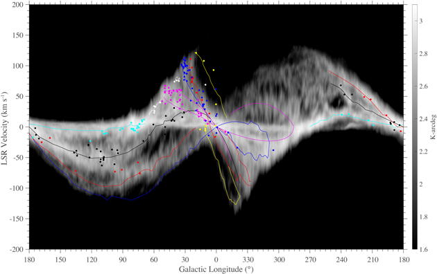
Figure 3. H i emission in gray scale as a function of and Galactic longitude. Colored dots are sources with parallax measurements shown in Fig 1 and the colored lines trace the spiral arms updated from Reid et al. (2016) and discussed in Section 3.2. Note we have connected the somewhat irregular () locations of giant molecular clouds seen in CO or H i emission, giving the slightly jagged spiral arm traces. The H I emission is from the Leiden/Argentine/Bonn survey of Kalberla et al (2005) and is integrated over the central 10 degrees of Galactic latitude.


Download figure:
Standard image High-resolution imageWe fitted log-periodic spirals to the locations of the masers, expanding upon the approach described in Reid et al. (2014). We now allow for a "kink" in an arm, with different pitch angles on either side of the kink. The basic form of the spiral model is given by

where R is the Galactocentric radius at a Galactocentric azimuth β in radians (defined as 0 toward the Sun and increasing in the direction of Galactic rotation) for an arm with a radius Rkink at a "kink" azimuth βkink. An abrupt change in pitch angle, , at βkink allows for a spiral arm to be described by segments, as found in large-scale simulations by D'Onghia et al. (2013), who suggest that spiral arms are formed from multiple segments that join together. Kinks are also observed in spiral galaxies, for example, by Honig & Reid (2015), who found that arm segments have characteristic lengths of 5–8 kpc, often separated by kinks or gaps. Since we currently have parallax measurements that trace arms over typically ≲12 kpc in length, allowing for only one kink is a reasonable simplification. When assigning kink locations we often relied on apparent gaps in the spiral arms.

In order to extend arm fits into the fourth Galactic quadrant (awaiting parallax measurements from southern hemisphere VLBI arrays), we constrain the fitted arms to pass near observed enhancements of CO and H i emission at spiral arm tangencies. Priors for these tangencies are listed in the notes for Table 2.
Table 2. Spiral Arm Characteristics
| Arm | N | ℓ Tangency | β Range | βkink | Rkink | ψ< | ψ> | Width |
|---|---|---|---|---|---|---|---|---|
| (deg) | (deg) | (deg) | (kpc) | (deg) | (deg) | (kpc) | ||
| 3 kpc(N) | 3 | 337.0 | 15 → 18 | 15 | 3.52 ± 0.26 | −4.2 ± 3.8 | −4.2 ± 3.8 | 0.18 ± 0.05 |
| Norma | 11 | 327.5 | 5 → 54 | 18 ± 4 | 4.46 ± 0.19 | −1.0 ± 3.3 | 19.5 ± 5.1 | 0.14 ± 0.10 |
| Sct–Cen | 36 | 306.1 | 0 → 104 | 23 | 4.91 ± 0.09 | 14.1 ± 1.7 | 12.1 ± 2.4 | 0.23 ± 0.05 |
| Sgr–Car | 35 | 285.6 | 2 → 97 | 24 ± 2 | 6.04 ± 0.09 | 17.1 ± 1.6 | 1.0 ± 2.1 | 0.27 ± 0.04 |
| Local | 28 | ... | −8 → 34 | 9 | 8.26 ± 0.05 | 11.4 ± 1.9 | 11.4 ± 1.9 | 0.31 ± 0.05 |
| Perseus | 41 | ... | −23 → 115 | 40 | 8.87 ± 0.13 | 10.3 ± 1.4 | 8.7 ± 2.7 | 0.35 ± 0.06 |
| Outer | 11 | ... | −16 → 71 | 18 | 12.24 ± 0.36 | 3.0 ± 4.4 | 9.4 ± 4.0 | 0.65 ± 0.16 |
Note. Spiral parameters from fitting log-periodic spirals for arms listed in column 1, based on data from Table 1. The number of massive young star parallaxes assigned to individual arms is given in column 2. Priors for Galactic longitudes of arm tangencies in quadrant 4 from Bronfman et al. (2000) (3 kpc(N): 337°; Norma: 328°; Sct–Cen: 308°; Sgr–Car: 283°) with uncertainties of ±2° were used to constrain fits in regions where few parallaxes have been measured; column 3 lists posteriori values from the fits. Column 4 gives the range of Galactocentric azimuth for the parallax data. The spiral model allowed for a "kink" at azimuth βkink (column 5) and radius Rkink (column 6), with pitch angles ψ< (column 7) and ψ> (column 8) for azimuths ≤ and >βkink, respectively. If βkink is given without uncertainty, it was not solved for and assigned a value based primarily on a gap in sources. If ψ< = ψ> , only a single pitch angle was solved for. Column 9 is the intrinsic (Gaussian 1σ) arm width at Rkink, adjusted with the other parameters in the Markov chain Monte Carlo trials, which resulted in a χν2 ≈ 1. The models assume R0 = 8.15 kpc.
Download table as: ASCIITypeset image
As before, we fitted a straight line to [x, y] = [ using a Markov chain Monte Carlo (MCMC) approach, in order to estimate the parameters by minimizing the distance perpendicular to the best-fit line. Our model included an adjustable parameter giving the (Gaussian 1σ) intrinsic width of a spiral arm, , where (dw/dR) = 42 pc kpc−1 was adopted from Reid et al. (2014). The data were variance weighted by adding in quadrature the effects of parallax–distance uncertainty and the component of the arm width perpendicular to the arm. The arm-width parameter w(Rkink) was adjusted along with the other model parameters and resulted in a reduced near unity.
![$\beta ,\mathrm{ln}(R/{R}_{\mathrm{kink}})]$](https://content.cld.iop.org/journals/0004-637X/885/2/131/revision1/apjab4a11ieqn22.gif)


We first weighted the data by assuming uncertainties that had a probability density function (PDF) with Lorentzian-like wings, which makes the fits insensitive to outliers (see the "conservative formulation" of Sivia & Skilling 2006), in order to identify and then remove sources with >3σ residuals (see the discussions of individual arms for source names). Then we re-fitted assuming a Gaussian PDF, and the best-fitting parameter values are listed in Table 2. Based on this approach, we find evidence for significant kinks in the Norma, Sagittarius, and Outer arms, as discussed in Section 3.2. As an example of the improved quality of fits by adding a kink, we did three fittings for the Sagittarius–Carina arm: (1) solving for a constant pitch angle which gave χ2 = 34.1 for 32 degrees of freedom (dof); (2) solving for different pitch angles about a kink fixed at an azimuth of 52° which gave χ2 = 30.9 for 31 dof; and (3) also solving for the kink azimuth, which gave a value of 24° with a χ2 = 25.5 for 30 dof.
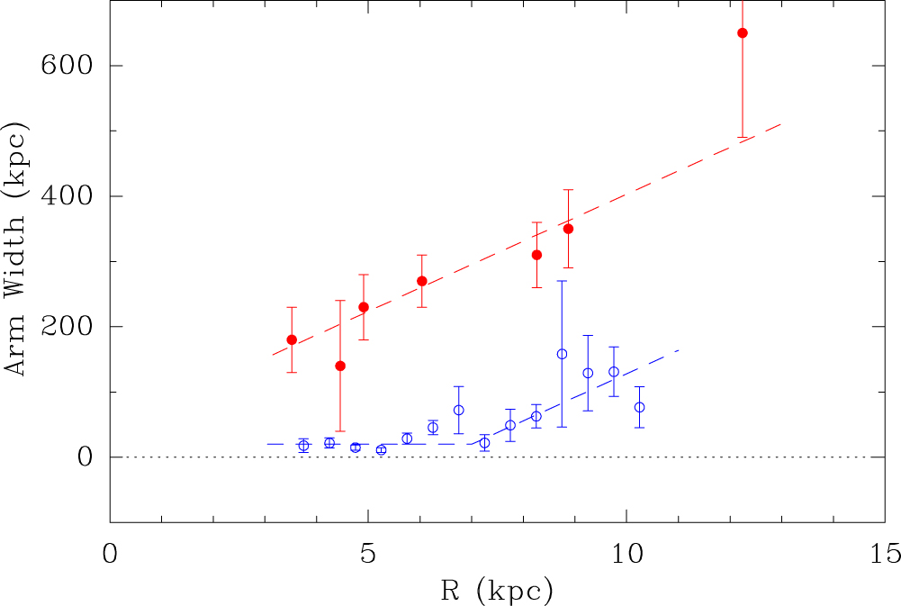
The best-fitting arm widths in the Galactic plane are plotted versus radius in Figure 4, extending the radial range and updating the results of Reid et al. (2014). We find that spiral arms widen with Galactocentric radius as pc.


Figure 4. Widths of spiral arms in the plane (red dots) and perpendicular to the plane (blue circles) as a function of Galactocentric radius. The in-plane widths represent averages over the 3 kpc, Norma, Scutum, Sagittarius, Local, Perseus, and Outer segments (in order of increasing average radius). The dashed red line is a best-fit straight line with a width of 336 pc at 8.15 kpc radius and a slope of 36 pc kpc−1. The out-of-plane widths are rms values after removing the effects of warping. The dashed blue line is a "by-eye" fit.
Download figure:
Standard image High-resolution image3.1. Distributions Perpendicular to the Plane
The distribution perpendicular to the Galactic plane of the young high-mass stars with maser emission is shown in the top panel of Figure 5. Plotted are true Z-heights, adjusted for the Sun's vantage point at 5.5 pc above the plane, but with no correction for the warping of the plane. The increasing scatter in Z beyond ≈6–7 kpc from the Galactic center is a combination of intrinsic scatter and the effects of warping. The lower panel of Figure 5 is a zoomed view of the inner 8 kpc. It reveals a very flat distribution with no sign of corrugations with amplitudes in excess of ≈10 pc. This is in contrast to H i observations toward tangencies in the inner Galaxy by Malhotra (1995), which suggest corrugations with semi-amplitudes of ≈30 pc.
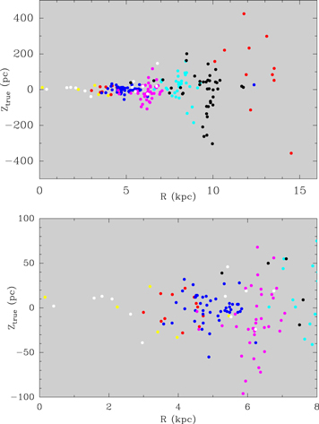
Figure 5. True Z-distribution of young high-mass stars perpendicular to the Galactic plane as a function of Galactocentric radius. Sources are color-coded by spiral arm as in Figure 1, and Ztrue values are corrected for our view from 5.5 pc above the plane, assuming the orientation of the IAU plane. Top panel: all stars in Table 1 with Galactocentric radii less than 16 kpc. Bottom panel: a zoomed view of sources within R = 8 kpc and ∣Z∣ < 100 pc.
Download figure:
Standard image High-resolution imageIn order to estimate the widths of arms perpendicular to the Galactic plane, one needs to deal with the effects of warping. We did this by smoothing the Z-heights along each arm with a window of ±20° of Galactic azimuth centered on each source. Provided there were at least five sources within the window, we then subtracted the variance-weighted mean-z. In order to minimize the effects of outliers, we iterated this process, removing 6σ, 5σ, 4σ, and finally 3σ outliers. Finally, with the effects of warping removed, the data from all arms were placed into 0.5 kpc bins in radius and rms values calculated. These rms values are displayed in Figure 4. These Z-widths can be reasonably described by pc, for R > 7.0 kpc, and constant at 20 pc inside that radius.

3.2. Updated Spiral Arm Model
Compared to Reid et al. (2014), we now have nearly double the number of young massive stars with maser parallaxes. Based on these data, the arms can be more clearly traced and some have been extended. Notable additions are spurs between the Local and Sagittarius arms (Xu et al. 2016) and between the Sagittarius and Scutum arms (B. Hu et al. 2019, in preparation). Figure 1, in addition to plotting the locations of stars with measured parallaxes, shows traces of four spiral arms and some arm segments and spurs. We now describe details of the observational constraints used to generate individual arm models.
3.2.1. Norma–Outer Arm
The Norma arm in the first quadrant displays a quasi-linear, spur-like structure, as seen in Figure 1, starting at (X, Y) = (3,2) kpc near the end of the bar and extending to about (2,5) kpc at Galactic azimuth of ≈18°. This segment of the arm has a large pitch angle of ≈20°. Proceeding counter-clockwise from that azimuth, in order to pass through the observed tangency in the fourth quadrant at ℓ ≈ 328°, the pitch angle of this segment must be near zero. Most likely the Norma arm wraps around the far side of the Galactic center and becomes the Outer arm as shown in Figure 1, where we have adjusted their pitch angles to join them together. Were the Norma arm instead to connect to the Perseus arm, it would have to have a negative pitch angle over a large azimuthal range, starting at (or beyond) the Norma tangency in the fourth quadrant. Alternatively, were it to connect to the Outer–Scutum–Centaurus (OSC) arm, it would need a very large pitch angle starting at (or beyond) the tangency. While neither of these possibilities seems likely, in order to rule them out parallaxes to some Norma–Outer arm sources beyond the Galactic center are needed. Note that we removed one outlier source (G001.15−0.12) when fitting spiral segments.
The Outer arm appears to have a kink in the second quadrant near Galactocentric azimuth 18° with a near-zero pitch angle as it proceeds into the third quadrant. The motivation for such a kink is based in part on a revised distance for S269. A new and robust BeSSeL Survey distance to S269 of 4.15 ± 0.22 kpc, from a 16-epoch set of observations (Quiroga-Nuñez et al. 2019), resolves the difference in parallax between VERA results by Honma et al. (2007) and Asaki et al. (2014) in favor of the latter result. With this new information, it appears likely that two other sources (G160.14+03.15 and G211.59+01.05) previously thought to lie between the Perseus and Outer arm, are likely part of an Outer arm segment which does not continue the pitch angle from the first and second quadrants into the third quadrant. This revision of the structure of the Outer arm is shown in Figure 1.

3.2.2. Scutum–Centaurus–OSC Arm
The Scutum arm may originate near β ≈ 90° in the first quadrant, and then wind counter-clockwise into the fourth quadrant as the Centaurus arm with a tangency at ≈306°. Over this large range of azimuth, one can reasonably fit a spiral with a pitch angle of ≈13°, since fitted pitch angles around a potential kink near 23° azimuth are statistically consistent (see Table 2). The fits in the table excluded six sources (G030.22−0.17, G030.41−0.23, G030.74−0.04, G030.81−0.05, G030.97−0.14, G031.41+0.30), which have unusually large proper motions (K. Immer et al. 2019, in preparation) and may be located in a spur-like structure.
As discussed by Sanna et al. (2017), extending this model beyond the Galactic center, it passes near the parallax source G007.47+00.05 and back into the first quadrant as the OSC arm (Dame & Thaddeus 2011; Sun et al. 2015). The association of the Scutum–Centaurus and OSC arm segments is pivotal information for a complete picture of the Milky Way, since it provides strong motivation for connecting the Norma and Outer arms, as both are directly interior to the Scutum–Centaurus–OSC arm. Were we not to connect the Scutum–Centaurus and OSC arm segments, it would require adding a fifth spiral arm tightly packed in a region that is difficult to measure. Occam's razor suggests that we adopt the four-arm approach.
3.2.3. Sagittarius–Carina Arm
In Figure 1, the Sagittarius arm has a 2 kpc long gap centered at azimuth β ≈ 24° near (X, Y) = (2,6) kpc. When fitting spiral segments, we removed two outliers (G032.74−0.07, G033.64−0.22). We found the best-fitting pitch angle for sources with β > 24° to be nearly zero (i.e., ψ = 10 ± 21). The arm segment for β < 24° in the first to the fourth quadrant tangency near β = −33° appears to have a pitch angle of ≈17°, based on the locations of parallax sources as well as its fourth quadrant tangency. This results in a significant kink, which was first suggested in a prescient paper by Burton & Shane (1970) and has appeared in models of the Milky Way, such as in the electron density model of Taylor & Cordes (1993). Beyond the fourth quadrant tangency, where we currently have no parallax information, we decrease the pitch angle to 10° in order to match the CO trace of the Carina arm, assuming kinematic distances (see Figure 3). Invoking symmetry with the Norma arm, we extend the Sagittarius arm inward to the Galactic bar near (−3, −3) kpc.

3.2.4. Perseus Arm
The Perseus arm has been thought to be one of two dominant spiral arms (along with the Scutum–Centaurus arm) of the Milky Way (Drimmel 2000; Churchwell & Benjamin 2009). While the arm has a large number of massive star-forming regions in the second quadrant, it appears to weaken and possibly die out in the 3rd quadrant (Koo et al. 2017). Also, spiraling inward and through the 1st quadrant, there is a clear decrease in active star formation (Zhang et al. 2013, 2019) extending for about 8 kpc along the arm between longitudes of 90° and 50°. Spiral pitch angles in each quadrant are similar and near 9°. Extrapolating the arm with this pitch angle inward into the fourth quadrant, it passes radially near but outside the bar and may originate near (X, Y) = (−3.5, −0.5) kpc as depicted in Figure 1. If this picture is correct, the Perseus arm is not a dominant arm as measured by high-mass star formation activity over most of its length.
3.3. Other Arm Segments
The Local arm has been mapped in detail by Xu et al. (2013, 2016). It appears to be an isolated arm segment with very significant massive star formation. However, it has not linked up with other segments to form a "true" arm, like those listed above, which can wrap fully around the Galaxy. Since we have only just begun to trace the 3 kpc and Connecting arms with parallax measurements, their natures are not yet well defined. However, these "arms" are associated with the Galactic bar and may not be true spiral arms.
4. Modeling the Galaxy
In order to estimate the distance to the Galactic center and rotation curve parameters, we used the Bayesian MCMC approach described in Reid et al. (2014). We treat as data the three-dimensional components of velocity and model these as arising from an axisymmetric Galactic rotation, allowance for an average streaming (non-circular) motion in the plane of the Galaxy. Previously, we adopted the "universal" form for the rotation curve (URC) of Persic et al. (1996), since it fitted the data as well as or better than other rotation curves, and it well models the rotation of a large number of external spiral galaxies. In our previous paper, we used a three-parameter formulation for the URC: , , and , where Ropt and are the radius enclosing 83% of the optical light and the circular velocity at that radius for a galaxy with luminosity L relative to an galaxy with mag. However, Persic et al., in their note added in proof, present a simplified two-parameter formulation with parameter a1 removed via scaling relations between optical radius, velocity, and luminosity. Since the two- and three-parameter formulations produce similar rotation curves over radial ranges of 0.5–2.0 Ropt, we now adopt the two-parameter version, with the rotation curve defined by only parameters a2 and a3. (See Appendix B for a FORTRAN subroutine that returns a circular rotation speed for a given Galactocentric radius.)


As in Reid et al. (2014), given the current uncertainty in the value for the circular component () of solar motion and the magnitude of the average peculiar motions of masers associated with massive young stars, we present fits with four sets of priors:

- (A)adopting a loose prior for the component of solar motion, , , km s−1, and for the average peculiar motion for the masing stars of and km s−1;
- (B)using no priors for the average peculiar motion of the stars, but a tighter prior for km s−1 from Schoenrich et al. (2010);
- (C)using no priors for the solar motion, but tighter priors on the average peculiar motion of the stars of and km s−1;
- (D)using essentially no priors for either the solar motion or average peculiar motion of the stars, but bounding the and parameters with equal probability within ±20 km s−1 of the set-A values and zero probability outside that range.


Since we expect large non-circular motions in the vicinity of the Galactic bar, we removed the 19 sources that are within 4 kpc of the Galactic center. Next, we removed 22 sources whose fractional parallax uncertainties exceeded 20%, in order to avoid significant complications arising from highly asymmetric PDFs when inverting parallax to estimate distance (e.g., Bailer-Jones 2015). Finally, as discussed in Reid et al. (2014), we expect some outliers in the motion data, owing for example to the effects of super-bubbles that can accelerate gas which later forms the stars with the masers we observe. Therefore, we used the "conservative formulation" of Sivia & Skilling (2006), which uses a "Lorentzian-like" PDF for motion uncertainties when fitting a preliminary model of Galactic rotation to the data. The best-fitting parameters are listed in Table 3 in column A1. This fit is largely insensitive to outliers, and allows us to identify and remove them in a prescribed and objective manner. Defining an outlier as having greater than a 3σ residual in any motion component, we removed 11 sources from further consideration.16
Table 3. Bayesian Fitting Results
| A1 | A5 | B | C | D | |
|---|---|---|---|---|---|
| Fitted Parameters | |||||
| R0 (kpc) | 8.22 ± 0.22 | 8.15 ± 0.15 | 8.15 ± 0.14 | 8.04 ± 0.17 | 8.04 ± 0.19 |
| (km s−1) | 10.8 ± 1.2 | 10.6 ± 1.2 | 10.7 ± 1.2 | 8.1 ± 2.5 | 8.2 ± 2.8 |
| (km s−1) | 13.6 ± 6.7 | 10.7 ± 6.0 | 11.9 ± 2.1 | 10.7 ± 4.8 | 6.5 ± 8.4 |
| (km s−1) | 7.6 ± 0.9 | 7.6 ± 0.7 | 7.7 ± 0.7 | 7.9 ± 0.8 | 7.9 ± 0.9 |
| (km s−1) | 6.1 ± 1.9 | 6.0 ± 1.4 | 6.2 ± 1.5 | 3.6 ± 2.6 | 3.7 ± 3.0 |
| (km s−1) | −2.1 ± 6.5 | −4.3 ± 5.6 | −3.1 ± 2.2 | −4.4 ± 4.5 | −8.7 ± 7.9 |
| a2 | 0.96 ± 0.08 | 0.96 ± 0.05 | 0.95 ± 0.05 | 0.95 ± 0.05 | 0.96 ± 0.05 |
| a3 | 1.62 ± 0.03 | 1.62 ± 0.02 | 1.62 ± 0.02 | 1.61 ± 0.02 | 1.62 ± 0.03 |
| Calculated Values | |||||
| (km s−1) | 237 ± 8 | 236 ± 7 | 236 ± 5 | 233 ± 6 | 238 ± 8 |
| ( + ) (km s−1) | 249 ± 7 | 247 ± 4 | 247 ± 4 | 244 ± 5 | 244 ± 6 |
| ( + )/R0(km s−1 kpc−1) | 30.46 ± 0.43 | 30.32 ± 0.27 | 30.32 ± 0.28 | 30.39 ± 0.28 | 30.36 ± 0.28 |
| Fit Statistics | |||||
| 809.7 | 425.0 | 427.3 | 426.2 | 425.7 | |
| Ndof | 465 | 432 | 432 | 432 | 432 |
| Nsources | 158 | 147 | 147 | 147 | 147 |
| 0.57 | 0.45 | 0.80 | 0.63 | 0.36 | |


Note. Fit A1 used the 158 sources in Table 1 with Galactocentric radii >4 kpc and fractional parallax uncertainty <20%, an "outlier tolerant" probability distribution function for data uncertainty (see Section 4), and set-A priors: Gaussian solar motion priors of , , km s−1 and average source peculiar motion priors of and km s−1. Fit A5 removed 12 sources found in Fit A1 to have a motion component residual greater than 3σ, and used a Gaussian probability distribution function for the residuals (ie, least-squares), and the same priors as A1. Fits B, C, and D were similar to A5, except for the priors: B used the solar motion priors of Schoenrich et al. (2010) km s−1 and no priors for source peculiar motions; C used no solar motion priors and source peculiar motion priors of and km s−1; D used flat priors for all parameters, except and which were given unity probability between ±20 km s−1 of the set-A prior values and zero probability outside this range. The fit statistics listed are chi-squared (), the number of degrees of freedom (Ndof), the number of sources used (Nsources), and the Pearson product-moment correlation coefficient for parameters R0 and ().


Download table as: ASCIITypeset image
With the resulting "clean" data set of 147 sources, we assumed a Gaussian PDF for the data uncertainties (equivalent to least-squares fitting) and the best-fitting parameter values are given in Table 3 in column A5. Note that we present estimates of in Table 3, calculated from the rotation curve, even though it was not a fitted parameter. We also combine parameters to generate the marginalized PDF for the full circular rotation rate of the Sun in linear, (+), and angular, (+)/R0, units. We adopt the A5 fit as the best model. However, for completeness we follow Reid et al. (2014) and also present model fits using the different priors listed above. Table 3 summarizes the best-fitting parameter estimates for priors B, C, and D in the last three columns, which yield parameter values similar to those for fit A5. Note that Quiroga-Nuñez et al. (2017) have shown that fits of mock data sets demonstrate that parameter estimates should be unbiased.


The correlation between parameters R0 and in fit A5 is modest: . This is similar to our previous value reported in Reid et al. (2014), as well as found in simulations by Quiroga-Nuñez et al. (2017), since it depends on the range and distribution of parallax sources, which has not significantly changed. Parallax measurements from a VLBI array in the southern hemisphere are needed to further reduce this correlation. As we have previously noted, , and can be highly correlated, hence the need for priors for some of these parameters. For the set-A priors, we find the following correlations: , , and .


5. Peculiar Motions
Using the Galactic parameters and solar motion values from fit A5, we can transform to a reference frame that rotates as a function of radius within the Galaxy. The resulting non-circular or peculiar motions in the plane of the Galaxy are shown in Figure 6. We only plot sources whose motion uncertainties are km s−1. While the vast majority of sources have moderate peculiar motions of ≲10 km s−1, we can identify two regions in the Galaxy with significantly larger peculiar motions. The first anomalous region is in the Perseus arm at Galactic longitudes between about and . This anomaly has been well documented in the literature (e.g., Humphreys 1978; Xu et al. 2006; Sakai et al. 2019). The second anomalous region is within a Galactocentric radius of . Large peculiar motions are seen near the end of the long bar for sources in the 3 kpc, Norma, and Scutum arms.


Figure 6. Non-circular (peculiar) motions of massive young stars in the plane of the Galaxy, adopting fit-A5 values for Galactic rotation and solar motion, without removing average streaming motions (i.e., setting ). Only sources with vector uncertainties km s−1 are shown. A 50 km s−1 scale vector is shown in the lower-right corner. Sources are color coded by arm as in Figure 1. A schematic "long" bar from Wegg et al. (2015) is indicated with the shaded ellipse.


Download figure:
Standard image High-resolution imageThe average peculiar motion of our sources for all fits in Table 3 indicates small positive values for (toward the Galactic center) and small negative values for (in the direction of Galactic rotation), possibly resulting from streaming motions of massive young stars toward the Galactic center and counter to Galactic rotation. Adopting fit A5, which has loose priors for the solar motion component in the direction of Galactic rotation ( km s−1) and for and (3 ± 10 and −3 ± 10 km s−1, respectively), we find and km s−1. The value appears significant and qualitatively consistent with theoretically expected values for the formation of stars from gas that was shocked when entering a spiral arm of low pitch angle (e.g., Roberts 1969).


6. The Galactic Plane
Given a source's distance and Galactic coordinates, we can calculate its three-dimensional location in the Galaxy. Since one expects massive young stars to be distributed very closely to the plane, this offers an opportunity to refine the parameters of the IAU-defined Galactic plane, as recently investigated by Anderson et al. (2019). Here we fit for the Sun's location perpendicular to the plane and a two-dimensional tilt of the true plane with respect to the IAU-defined plane. Then, with improved parameters, we estimate the scale height of our sources.
We define Cartesian Galactocentric coordinates , where X is distance perpendicular to the Sun–Galactic center line (positive in the first and second quadrants), Y is distance from the Galactic center toward the Sun, and Z is distance perpendicular to the plane (positive toward the north Galactic pole). In order to avoid complications of Galactic warping, we follow Gum et al. (1960) and Blaauw et al. (1960) and restrict the range of sources fitted to within a Galactocentric radius of 7.0 kpc, giving a sample of 116 sources. Anticipating a scale height for massive young stars near 20 pc (see below), we also remove possible "outlying" sources more than 60 pc from the plane. Some outliers would be expected if gas compressed and accelerated by superbubbles forms high-mass stars. With these restrictions, we retained 96 massive young stars and plot their three-dimensional locations in the Galaxy relative to the IAU-defined plane in Figure 7.


Figure 7. Perspective plots of the three-dimensional locations (cone tips) of massive young stars with respect to the IAU-defined Galactic plane. Only 96 sources within 7 kpc of the center are shown to avoid regions of Galactic warping. Note the ZIAU scale is in pc, whereas the X and Y scales are kpc. Left is a view from 3 deg above the plane and right is from 3 deg below the plane. Two views are shown to better display the slight asymmetry in ZIAU favoring negative values, owing to our viewpoint from the Sun which is above the plane.
Download figure:
Standard image High-resolution imageThese stars are very tightly distributed in a plane. However, the distribution about the IAU-defined plane is slightly asymmetric, with two-thirds (65) of the sources lying below that plane. The mean offset is −7.3 pc with a standard error of the mean of ±2.1 pc. In general, this can be explained by a combination of the Sun being offset from the true Galactic plane and/or a tilt of the true plane from the IAU plane. Hence, we fitted an adjusted plane to these data. We treat the observed () values as data and model them as follows:


where is the Z-offset of the Sun, dp is the distance of a source from the Sun projected in the plane, l is Galactic longitude, and and are tilt angles of the true plane with respect to the IAU-defined plane (referred to as "roll" and "tilt," respectively, by Anderson et al. 2019). The data were fitted using an MCMC technique, accepting or rejecting trials with the Metropolis–Hastings algorithm. Data uncertainties were based on parallax uncertainties and assumed to be Gaussian. In order to minimize the effects of distance biases, owing to asymmetric distance PDFs when converting parallaxes to distances (e.g., Bailer-Jones 2015), we used only the 80 sources with fractional parallax uncertainties less than 20%.


Figure 8 displays the MCMC trials and marginalized PDFs for the three parameters. The centers of the 68% confidence ranges for the marginalized PDFs give the following parameter estimates: pc, , and . Thus, we find very small changes in the orientation ("tilt" parameters) of the true Galactic plane relative to the IAU-defined plane. Anderson et al. (2019) find similarly small values of (between and +015) and (between and +008) for different sub-samples. Therefore, for simplicity, in the following we assume the orientation of the plane follows the IAU definition, but we correct for the Sun's Z-height above the plane.


Figure 8. Results of fitting three parameters defining a tilted plane to the Galactic Z-heights of massive young stars within 7 kpc of the Galactic center. Plotted are two-dimensional 68% and 95% confidence contours based on the MCMC trial parameter values and their one-dimensional marginalized probability densities. ZSun is the offset of the Sun from the true plane toward the north Galactic pole; ϕX and ϕY are rotation angles of the true plane with respect to the IAU-defined plane about lines toward the Galactic center and toward 90° Galactic longitude, respectively.
Download figure:
Standard image High-resolution imagePlacing the Sun 5.5 pc above the IAU-defined plane, we calculate Z-offsets relative to the true (adjusted) Galactic plane, which we designate Ztrue. Figure 9 presents a binned histogram of Ztrue values for our full sample of 120 massive young stars within 7.0 kpc of the Galactic center and 200 pc of the plane, along with the best-fitting exponential distribution. The exponential distribution fits the data very well and gives a scale height of 19 ± 2 pc.

Figure 9. Histogram of distances perpendicular to the "true" Galactic plane after correcting for the Sun's location of 5.5 pc above the plane. In order to avoid the effects of warping, only sources within 7 kpc of the Galactic center are plotted. The dashed red line is the best-fitting exponential distribution with a scale height of 19 pc.
Download figure:
Standard image High-resolution image7. Precession of the Plane
We now investigate the possibility that the Galaxy precesses, possibly owing to torques from its triaxial halo and/or from Local Group galaxies. A rigid-body precession of the plane could be inferred from the Z-component of velocity of our massive young stars, Ws, following

where and are the speeds of vertical motion at radius R0 and location in the plane given by X and Y. We used the estimate of Schoenrich et al. (2010) of the vertical motion of the Sun relative to the solar neighborhood of km s−1 as a strong prior. After removing Ws measurements with uncertainties km s−1, we fitted the data using a Bayesian MCMC procedure similar to that described in Section 4, first using the "conservative formulation" of Sivia & Skilling (2006) to identify and remove 20 outliers and then refitting with Gaussian data uncertainties. Using sources at all Galactocentric radii, we find km s−1, km s−1, and km s−1. Dividing the data into inner and outer regions, we find for kpc, km s−1, km s−1, and km s−1, and for , km s−1, km s−1, and km s−1. The estimates of for the inner and outer Galaxy differ by 3.2 ± 1.7 km s−1 with nearly 2σ significance, hinting at the possibility of a radial dependence.


The Galaxy is known to exhibit significant warping, starting between about 7 and 8 kpc radius and reaching an amplitude of about 300 pc at a radius of 12 kpc (Gum et al. 1960). Since the warping is likely dynamic in origin, one would expect vertical motions leading the warp to vary with radius. Were the warping at 12 kpc radius to develop over a timescale of yr (roughly one-third of an orbital period at that radius), that would correspond to a characteristic vertical speed of ∼3 km s−1. In order to investigate this possibility, we added second-order terms to Equation (1) yielding


Re-fitting with no radial restriction, we find km s−1, km s−1, km s−1, km s−1, and km s−1. Neither the first- nor second-order parameters differ significantly from zero, and for the y-terms reasonable upper limits for their magnitudes (and hence for vertical motions at ) are km s−1.


8. Discussion
8.1. An Updated View of the Milky Way
Is the Milky Way a two- or four-arm spiral? Based on the model described in Section 3.2, the answer is a four-arm spiral as traced by massive young stars. The four arms do not include sub-structures such as the 3 kpc arms, since they are likely a phenomenon associated with the bar, and the Local arm, which appears to be an isolated segment. Were the Milky Way a two-arm spiral, its arms would have to wrap twice around the center in order to accommodate the parallax data. This would require pitch angles to average near 5°. However, based on the data in Table 2 and weighting the pitch angles by their segment lengths, we find an average pitch angle of 10° for the major arms (Norma–Outer, Sct–Cen–OSC, Sgr–Car, and Perseus).
The form of spiral arm segments obtained in Section 3.2 can be used to update the input model for the parallax-based distance estimator of Reid et al. (2016) (see Appendix A for details). Coupling our revised model of spiral arm locations with line-of-sight velocities that trace arms in CO or H i emission in longitude–velocity plots, we arrive at a revised spatial-kinematic model for arms. Incorporating the revised arm model into our parallax-based distance estimator, we can now take longitude–latitude–velocity values from surveys of spiral-arm tracers (e.g., H ii regions, molecular clouds, star-forming masers) and estimate distances more accurately than from standard kinematic distances. Taking as input the catalogs of water masers from Valdettaro et al. (2001), methanol masers from Pestalozzi et al. (2005) and Green et al. (2017), H ii regions from Anderson et al. (2012), and red MSX sources from Urquhart et al. (2014), we now construct an improved visualization of the spiral structure of the Galaxy, shown in Figure 10.

Figure 10. Plan view of the Milky Way showing the locations of high-mass star-forming regions estimated using version 2 of the parallax-based distance estimator of Reid et al. (2016). Sources for which the distance estimator could reasonably assign to an arm are shown in blue, otherwise they are in cyan. The Galactic center (red asterisk) is at (0,0) and the Sun (red Sun symbol) is at (0,8.15) kpc. The wedge-shaped region between dashed lines suffers from incompleteness as discussed in the text. The background gray spirals are based on the parameters in Table 2, with small adjustments to allow arm segments to connect smoothly beyond the Galactic center, and have widths of 1.65σ, which would enclose 80% of sources assuming a Gaussian distribution perpendicular to the arms. The "long" bar is indicated with the shaded ellipse.
Download figure:
Standard image High-resolution imageWhile the locations of spiral arms can be obtained from a sample of maser parallaxes that is far from complete, the input catalogs for our visualization of the Milky Way have better defined samples and are more complete. For example, the red MSX catalog of Urquhart et al. (2014) is estimated to be complete for star-forming regions with bolometric luminosities to a distance of 18 kpc. While the map in Figure 10 should be much more complete than that in Figure 1, we suspect that it under-represents distant sources, owing to their intrinsic weakness as well as effects of confusion. Therefore, as a first attempt to correct for incompleteness, for sources more distant than 3 kpc we randomly "sprinkle" a number of points given by (capped at 10 points) from a Gaussian distribution whose width increases with Galactocentric radius as found in Section 3.


The visualization of the pattern of sources associated with spiral arms in Figure 10 shows a dearth of sources toward the Galactic center within a cone of half angle . This is likely a result of survey bias against identifying distant, weak sources in the presence of numerous strong nearby sources. Also, most sources in the general direction of the Galactic center have LSR velocities close to zero, which can limit the information used to discriminate among arm assignments.

8.2. Fundamental Galactic Parameters
The distance to the Galactic center, R0, is a fundamental parameter affecting a wide variety of astrophysical questions (e.g., Reid 1993). As such there are a large number of estimates for R0, and we restrict our discussion to direct methods. A trigonometric parallax measurement of water masers from Sgr B2, a massive star-forming region within pc of the Galactic center, indicates (Reid et al. 2009c). The most recent analyses of infrared observations tracing the orbits of stars around the supermassive black hole, Sgr A*, provide geometric estimates of R0 of 7.946 ± 0.059 kpc (Do et al. 2019) and 8.178 ± 0.026 kpc (Gravity Collaboration et al. 2019), where the improved accuracy of the latter measurement comes from infrared interferometric observations. Our result of is both independent of, and consistent with, these estimates.


While there are moderate correlations among R0, , and , our parallax data strongly constrain the linear and angular speeds of the Sun in its Galactic orbit. Adopting the A5-fit results, we find km s−1 and km s−1 kpc−1. This can be compared to an independent and direct estimate from the apparent proper motion of the supermassive black hole, Sgr A*, assuming it is stationary at the center of the Milky Way. Reid & Brunthaler (2004) measure the apparent motion of Sgr A* in Galactic longitude to be −6.379 ± 0.019 mas yr−1. This implies km s−1 kpc−1. Thus, our estimate of the angular orbital speed of the Sun is in excellent agreement with the apparent proper motion of Sgr A*.


Our best-fit model rotation curve for the Galaxy (fit A5) is shown in Figure 11 as the dotted–dashed line. This curve has the URC form and is specified by only two parameters ( and ). The slight bias of the curve above the data is a result of the tendency for massive young stars to lag Galactic rotation with km s−1. This rotation curve peaks at 237 km s−1 at a radius of 6.8 kpc and falls to 227 km s−1 at a radius of 14.1 kpc, corresponding to a slope of 1.4 km s−1 kpc−1 or, alternatively, with a power-law index of −0.059 over that radial range.


Figure 11. Rotation curve for masers associated with massive young stars based on measured parallaxes and proper motions. Plotted is the circular velocity component, Θ, as a function of Galactocentric radius, R. Top panel: the transformation from heliocentric to Galactocentric frames uses the parameter values of fit A5, which is based on sources plotted with filled red symbols. Sources not used in fit A5 with R < 40 kpc are plotted with open blue symbols and outliers (see the text for details) are plotted with open green symbols. The dashed–dotted red line is the fitted two-parameter "universal" rotation curve for spiral galaxies (Persic et al. 1996), allowing for an average lag of 4.3 km s−1 for massive young stars. Bottom panel: the filled black points are variance-weighted averages of the data used in the fitting (adjusted for the average lag) and smoothed with a boxcar window of 1.0 kpc full-width.
Download figure:
Standard image High-resolution imagePlotted with black dots in the lower panel of Figure 11 are variance-weighted averages of the data, after correcting for the lag, within a window of 1 kpc full-width in steps of 0.25 kpc (see Table 4). This model-independent rotation curve shows only a very slight departure from the URC model. The data could support a small decrease of ≈5 km s−1 between radii of 7 to 9 kpc, followed by a flattening out to 10 kpc. However, there is no evidence for a ≈20 km s−1 dip in the rotation curve near R = 9 kpc with a width of ≈2 kpc, as has been suggested in the literature (e.g., Sofue et al. 2009). Qualitatively, our rotation curve is similar to that presented in the review by Bland-Hawthorn & Gerhard (2016) and more recently in the paper by Eilers et al. (2019) (allowing for their estimate of of 229 km s−1, which is 7 km s−1 below our value).

Table 4. Rotation Curve
| R (kpc) | ||
|---|---|---|
| 0.250 | 50.73 | ... |
| 0.500 | 77.36 | ... |
| 0.750 | 98.72 | ... |
| 1.000 | 116.96 | ... |
| 1.250 | 132.93 | ... |
| 1.500 | 147.06 | ... |
| 1.750 | 159.61 | ... |
| 2.000 | 170.76 | ... |
| 2.250 | 180.64 | ... |
| 2.500 | 189.38 | ... |
| 2.750 | 197.07 | ... |
| 3.000 | 203.80 | ... |
| 3.250 | 209.67 | ... |
| 3.500 | 214.73 | ... |
| 3.750 | 219.09 | ... |
| 4.000 | 222.79 | 224.06 ± 2.72 |
| 4.250 | 225.93 | 227.82 ± 1.81 |
| 4.500 | 228.54 | 228.10 ± 1.63 |
| 4.750 | 230.70 | 230.36 ± 1.62 |
| 5.000 | 232.46 | 233.51 ± 1.40 |
| 5.250 | 233.87 | 234.60 ± 1.52 |
| 5.500 | 234.97 | 236.25 ± 1.42 |
| 5.750 | 235.81 | 239.46 ± 1.19 |
| 6.000 | 236.41 | 239.88 ± 1.22 |
| 6.250 | 236.82 | 240.30 ± 1.14 |
| 6.500 | 237.06 | 240.38 ± 1.07 |
| 6.750 | 237.16 | 239.32 ± 1.17 |
| 7.000 | 237.14 | 238.53 ± 1.24 |
| 7.250 | 237.02 | 238.01 ± 1.41 |
| 7.500 | 236.82 | 234.57 ± 1.41 |
| 7.750 | 236.55 | 232.82 ± 1.08 |
| 8.000 | 236.23 | 232.83 ± 1.00 |
| 8.250 | 235.87 | 232.67 ± 1.00 |
| 8.500 | 235.48 | 233.04 ± 1.05 |
| 8.750 | 235.06 | 231.99 ± 1.33 |
| 9.000 | 234.63 | 230.78 ± 1.66 |
| 9.250 | 234.19 | 231.41 ± 1.24 |
| 9.500 | 233.75 | 231.52 ± 1.15 |
| 9.750 | 233.30 | 232.08 ± 1.21 |
| 10.000 | 232.86 | 232.46 ± 1.22 |
| 10.250 | 232.42 | 233.21 ± 1.69 |
| 10.500 | 231.99 | 232.89 ± 3.15 |
| 10.750 | 231.57 | ... |
| 11.000 | 231.16 | ... |
| 11.250 | 230.76 | ... |
| 11.500 | 230.38 | 232.01 ± 6.11 |
| 11.750 | 230.01 | 225.85 ± 3.38 |
| 12.000 | 229.65 | 225.85 ± 3.38 |
| 12.250 | 229.31 | 224.66 ± 3.76 |
| 12.500 | 228.98 | ... |
| 12.750 | 228.67 | ... |
| 13.000 | 228.37 | ... |
| 13.250 | 228.08 | ... |
| 13.500 | 227.81 | ... |
| 13.750 | 227.54 | ... |
| 14.000 | 227.30 | ... |
| 14.250 | 227.06 | ... |
| 14.500 | 226.83 | ... |
| 14.750 | 226.62 | ... |
| 15.000 | 226.41 | ... |
| 15.250 | 226.22 | ... |
| 15.500 | 226.04 | ... |
| 15.750 | 225.86 | ... |
| 16.000 | 225.70 | ... |
| 16.250 | 225.54 | ... |
| 16.500 | 225.39 | ... |
| 16.750 | 225.25 | ... |
| 17.000 | 225.11 | ... |
| 17.250 | 224.98 | ... |
| 17.500 | 224.86 | ... |
| 17.750 | 224.74 | ... |
| 18.000 | 224.63 | ... |
| 18.250 | 224.53 | ... |
| 18.500 | 224.43 | ... |
| 18.750 | 224.33 | ... |
| 19.000 | 224.24 | ... |
| 19.250 | 224.16 | ... |
| 19.500 | 224.07 | ... |
| 19.750 | 224.00 | ... |
| 20.000 | 223.92 | ... |


Note. R is Galactocentric radius, is the universal rotation curve from fit A5, and are variance-weighted, circular velocities for the masers within a radial window of 1 kpc; these values have also been adjusted upward by 4.3 km s−1 to account for the average lag found in fit A5.


In the context of the URC formalism, , implying and , yielding . Persic et al. (1996) give a halo mass of , which returns , and a disk scale length .


Reid et al. (2014) examined the impact of revised Galactic parameters on the Hulse–Taylor binary pulsar's orbital decay, owing to gravitational radiation as predicted by general relativity (GR). This test of GR is sensitive to () accelerations from the Galactic orbits of the Sun and the pulsar. Repeating that analysis with the Galactic parameters of fit A5, we find that the binary's orbital decay rate is 0.99658 ± 0.00035 (nearly a 10σ deviation) of that expected from GR for the originally assumed pulsar distance of 9.9 kpc. However, we note that, using our estimates of the values and uncertainties in R0 and , a distance of 6.54 ± 0.24 kpc would remove the discrepancy from the GR prediction, providing a strong prediction that can be tested with a direct pulsar parallax measurement.


8.3. Displacement of the Sun from the Galactic Plane
In Section 6, we modeled the distances perpendicular to the IAU-defined Galactic plane (ZIAU) for our sample of massive young stars, allowing for the Sun's offset from the plane () and tilts of the true plane from the IAU-plane in the X and Y directions. We found no significant tilting within uncertainties of . This finding is consistent with the H i and radio continuum data used to define the (inner) plane with similar uncertainty (Gum et al. 1960). Were we to assume no uncertainty in the orientation of the IAU-plane, we would obtain pc. Allowing for the uncertainty in tilt of the true plane from the IAU-plane, we find the Sun's displacement is pc toward the north Galactic pole.


Our method to estimate is direct and simple, essentially averaging Z-values for extremely young and massive stars, which should tightly trace the Galactic plane. These are typically O-type stars which have recently formed or are still forming (≲105 yr). Their very small scale height of 19 pc attests to their being extreme Population I stars. All distances are determined by trigonometric parallax, and we only used measurements with uncertainties less than 20%, thus avoiding significant bias when converting parallax to distance. In contrast to optically based observations, which can be plagued by variable Galactic extinction, our radio observations are unaffected by extinction. Finally, we have restricted our analysis to Galactocentric radii in order to avoid serious complications from Galactic warping. One shortcoming of our sample might be that we have almost no sources in the fourth Galactic quadrant. However, H i observations have demonstrated little difference in the Z distribution between the first and fourth quadrants in the inner 7 kpc of the Galaxy (Gum et al. 1960).


How does our estimate of compare to previous values? First, we note that it agrees with the results based on H ii regions of Anderson et al. (2019), who provide a range of estimates for between 3 and 6 pc, assuming no tilt of the true plane with respect to the IAU-defined plane (see their Table 3), but a larger range when a tilt is allowed (see their Table 4). However, there is a very large scatter in estimates of in the literature, with most values ranging between about 5 and 40 pc (see, e.g., Bland-Hawthorn & Gerhard 2016). Interestingly, dividing the published results into three groups suggests systematic differences: (1) radio and infrared studies typically find pc (Gum et al. 1960; Pandy & Mahra 1987; Toller 1990; Cohen 1995; Binney et al. 1997); (2) optical studies of OB and other young massive stars give pc (Stothers & Frogel 1974; Pandy et al. 1988; Conti & Vacca 1990; Reid 1990); (3) optical star counts yield pc (Stobie & Ishida 1987; Yamagata & Yoshii 1992; Humphreys & Larsen 1995; Méndez and van Altena 1998; Chen et al. 2001; Maíz-Appelániz 2001; Jurić et al. 2008). The differences between group (1) and the other groups might be partially attributed to the effects of extinction, which complicates the optical measurements of groups (2) and (3). The differences between the two optical groups may be more subtle, but generally studies that are restricted to the solar neighborhood give larger estimates than those with a larger Galactic reach. These differences suggest that a combination of extinction and Galactic warping may be affecting the optical results.


Extinction is known to be irregular and could easily bias the ratio of star counts north and south of the Galactic plane, which is the basis for many estimates of . Changing the count ratio by 10% would change the estimates of Humphreys & Larsen (1995) and Chen et al. (2001) by about 15 pc and that of Yamagata & Yoshii (1992) by about 30 pc. Additionally, differences between solar neighborhood and Galactic scale studies might be attributed to the effects of warping of the Galactic plane. While the inner portion of the Galactic plane is known to be very flat, starting between about 7 and 8 kpc from the center, the Galaxy warps upward toward lII ≈ 50° and downward toward lII ≈ 310° (see Gum et al. 1960, noting their use of the old Galactic longitude system lI). Since this warping can reach 100 pc at a radius of about 9.7 kpc, it would not be surprising if star counts could be biased to yield estimates in error by ∼10 pc. Thus, it is critical to reference estimates to the inner plane of the Milky Way as we have done.


Finally, we note that our best-fit value for of 5.5 pc is very close to that needed to move the true Galactic center, defined by the location of the supermassive black hole Sgr A*, to its apparent latitude of (corresponding to pc relative to the IAU-plane at a distance of 8.15 kpc).


9. Concluding Remarks
The original five-year phase of the BeSSeL Survey used about 3500 hr on the VLBA. Results in this paper are nearly complete through the first four years of the project. The final year's observations, which preferentially targeted distant sources and those especially important to better define spiral arms, are currently being analyzed.
While Figure 10 presents the most complete picture of the spiral structure of the Milky Way to date, in regions lacking parallax data, distances to arm segments are necessarily less accurate. This model can be improved by adding parallaxes for sources in the fourth quadrant. In the near future, an extension of the BeSSeL Survey to the southern hemisphere is planned. Using the University of Tasmania's AuScope array of four antennas spanning the Australian continent (Yarragadee in Western Australia, Katherine in the Northern Territory, Ceduna in South Australia, and Hobart in Tasmania), agumented by an antenna in New Zealand (Warkworth), we anticipate starting observations in 2020. After several years of observation, we hope to obtain parallaxes for 50 to 100 6.7-GHz masers in the Galactic longitude range 240°–360°, where currently only a few have been measured.
In the long term, we would like to better explore the Milky Way well beyond its center, at distances of 10–20 kpc, in order to test and improve our current model of spiral structure. While some progress can be made with existing VLBI arrays, adding large numbers of parallaxes for these very distant regions may require the next generation of radio facilities, such as the SKA and ngVLA, with high sensitivity and long baselines.
This work was partially funded by the ERC Advanced Investigator Grant GLOSTAR (247078). It was also sponsored by the MOST grant No. 2017YFA0402701 and NSFC Grants 11933011, 11873019 and 11673066. B.Z. and Y.W.W. are supported by the 100 Talents Project of the Chinese Academy of Sciences (CAS). A.B. acknowledges support by the National Science Centre Poland through grant 2016/21/B/ST9/01455. K.L.J.R. acknowledges funding by the Advanced European Network of E-infrastructures for Astronomy with the SKA (AENEAS) project, supported by the European Commission Framework Programme Horizon 2020 Research and Innovation action under grant agreement No. 731016.
Facilities: VLBA - Very Long Baseline Array, VERA - , EVN - , Australian LBA. -
Appendix A
Version 2 of our parallax-based distance estimator (Reid et al. 2016), as well as the FORTRAN code and spiral arm data, can be found at http://bessel.vlbi-astrometry.org/. It incorporates the improved model for the locations of spiral arms in the Milky Way described in Section 3.2. The previous model only included the locations of arm segments in the first, second, and third Galactic quadrants. We now provisionally extend the arm models to the fourth quadrant by extrapolating arms interior to the solar circle from the first quadrant guided by the directions of arm tangencies in the fourth quadrant. We also assume that arms do not cross each other on the far side of the Galactic center, and we make use of the parallax measurement of G007.47+00.05 (Sanna et al. 2017), which ties the Scutum–Centaurus arm beyond the Galactic center with the "Outer–Scutum–Centaurus" arm. It then follows that the Norma arm connects with the Outer arm beyond the Galactic center, and that the Perseus arm is interior to the Norma arm, most likely originating near the far end of the Galactic bar. In addition, in Version 2 we include the following improvements.
- 1.Source coordinates can now be entered either as J2000 (R.A., decl.) or Galactic (). R.A. and decl. must be in hhmmss.s and ddmmss.s format, and the program assumes values smaller than 000360.0 and between ±000090.0 are Galactic coordinates in degrees, since such small values for both R.A. and decl. are far from the Galactic plane.
- 2.In Version 1, the spiral arm and Galactic latitude PDFs were plotted separately. Since the arm-assignment probability terms, , are distance independent and depend on Galactic latitude, not Z-height, they alone favor nearer arms over more distant arms. While this bias was corrected for by considering the distance-dependent Galactic latitude PDF (which uses Z-heights), for simplicity we now combine the sprial arm and Galactic latitude PDFs into a single PDF.
- 3.The uncertainty in can now be entered and included in the probability densities.
- 4.Proper motions in both Galactic longitude and latitude and their uncertainties, if measured, can now be entered and used to estimate distances. Given a rotation curve and proper motion components, one can calculate a distance PDF from the longitude motion in an analogous fashion to using Doppler velocities. This alternative type of "kinematic distance" (Yamauchi et al. 2016; Sanna et al. 2017) has no distance ambiguity and is most effective toward the Galactic center and anticenter, the directions in which conventional kinematic distances based on radial velocities are least effective. Also, for a given velocity dispersion perpendicular to the Galactic plane, the latitude motion should decrease with distance, and one can also obtain a distance PDF for this component of motion.
- 5.Since sources near the Galactic bar can exhibit large peculiar motions, we now inflate motion uncertainties for these sources in order to down-weight the impact of their kinematic distance PDFs. Starting inward from R = 6 kpc, we add a peculiar motion uncertainty in quadrature with measurement motion uncertainty. This peculiar motion uncertainty is zero at R = 6 kpc and increases linearly to 25 km s−1 at R = 4 kpc; inside of R = 4 kpc we hold it constant at 25 km s−1.
- 6.In addition to the Galactic bar region, large peculiar motions are seen for sources in the Perseus arm in the second quadrant within a region bounded by and . For sources within this reigon, we add 20 km s−1 in quadrature with measured uncertainties of each motion component.
- 7.For batch processing, the FORTRAN program now reads a source-information file that contains the information for each source on a single ascii-text line.


Appendix B
| subroutine Univ_RC_from_note (r, a2, a3, Ro, | ||
| + | Tr ) | |
| c | Disk plus halo parameterization of rotation curve... | |
| c | see Persic, Salucci and Stel 1996 Note Added in Proof | |
| c | Input parameters: | |
| c | r: Galactocentric radius in kpc | |
| c | a2: Ropt/Ro where Ropt=3.2∗R_scalelength encloses 83% of light | |
| c | a3: 1.5∗(L/L∗)o(1/5) | |
| c | Ro: Ro in kpc | |
| c | Output parameter: | |
| c | Tr: Circular rotation speed at r in km/s | |
| implicit real∗8 (a-h,o-z) | ||
| real∗8 lambda, log_lam | ||
| lambda=(a3/1.5d0)∗∗5 ! L/L∗ | ||
| Ropt=a2 ∗ Ro | ||
| rho=r/Ropt | ||
| c Calculate Tr... | ||
| log_lam=log10(lambda ) | ||
| term1=200.d0∗lambda∗∗0.41d0 | ||
| top=0.75d0∗exp(-0.4d0∗lambda) | ||
| bot=0.47d0+2.25d0∗lambda∗∗0.4d0 | ||
| term2=sqrt(0.80d0 + 0.49d0∗log_lam + (top/bot) ) | ||
| top=1.97d0∗rho∗∗1.22d0 | ||
| bot=(rho∗∗2 + 0.61d0)∗∗1.43d0 | ||
| term3=(0.72d0 + 0.44∗log_lam) ∗ (top/bot) | ||
| top=rho∗∗2 | ||
| bot=rho∗∗2+2.25∗lambda∗∗0.4d0 | ||
| term4 = 1.6d0∗exp(-0.4d0∗lambda) ∗ (top/bot) | ||
| Tr=(term1/term2) ∗ sqrt(term3 + term 4) ! km/s | ||
| return | ||
| end |
Download table as: ASCIITypeset image
Footnotes
- 14
- 15
- 16
G015.66−00.49, G029.86−00.04, G029.98+00.10, G030.19−00.16, G030.22−00.18, G030.41−00.23, G030.81−00.05, G032.74−00.07, G078.12+03.63, G108.59+00.49, G111.54+00.77.