Detection of Coronal Mass Ejections at L1 and Forecast of Their Geoeffectiveness

A geomagnetic storm is a severe disturbance of the Earth's magnetosphere caused by the strong interaction of the solar wind (a highly structured flow of plasma, magnetic field and particles coming from the Sun) with the Earth's magnetic field. The largest storms are due to coronal mass ejections (CMEs), large eruptions of magnetized plasma from the upper Sun's atmosphere—the solar corona—into the interplanetary space. CMEs reach speeds from hundreds up to a few thousands of km s⁻¹ (e.g., Sheeley et al. 1999), corresponding to transit times from several hours to several days. During their propagation CMEs expand in size, reaching radial extensions of about 0.25 au at Earth (Klein & Burlaga 1982). CMEs propagating faster than the magnetosonic speed in the frame of reference of the background solar wind drive the formation of a shock wave ahead of them (e.g., Raymond et al. 2000), which accelerates solar energetic particles (Reames 1999), potentially increasing the geomagnetic storm intensity. Other sources of geomagnetic disturbances are the high-speed streams (HSSs) and, to a lesser extent, the crossings of the heliospheric current sheet (HCS), namely the surface within the heliosphere where the Sun's magnetic field switches polarity. When HSSs overtake the slower solar wind in front of them, they create interaction regions characterized by very high densities and intense magnetic fields, known as corotating interaction regions (CIRs). CIRs can cause geomagnetic storms that, even if less intense than the CME-driven ones, can last for a longer time. Since space weather activity strictly depends also on the direction of the magnetic field advected by the solar wind, it turns out that also HCS crossings may impacts the Earth's magnetosphere.

Solar storms induce intense variations of the ring current in the magnetosphere (an electric current circling the Earth in the equatorial plane). The disturbance storm time (DST) index is an estimate of the ring current, hourly derived from a network of near-equatorial geomagnetic stations. DST can be thus used to classify geomagnetic storms as moderate (−50 nT > DST > −100 nT), intense (−100 nT > DST > −250 nT), or super (DST < −250 nT) storms (Cander & Mihajlovic 1998). Also the auroral currents in the auroral ionosphere (electric currents aligned to the Earth's magnetic field) are highly perturbed by solar storms. The planetary geomagnetic disturbance index Kp (or the equivalent Ap index), derived by a network of subauroral observatories, is a 3 hourly range measure of these currents. The Kp index is mainly designed to measure the geomagnetic storms by their effects, from minor (Kp = 5) to extreme (Kp = 9) events. The daily Ap* index, derived as the eight-point running average of successive 3 hr Ap indices, is usually used to establish the timing and duration of geomagnetic storm events. These are indeed identified when Ap* ≥ 40.

The energy released into the magnetosphere during geomagnetic storms drives an increase of the density in the Earth's upper atmosphere, which results in extra drag on satellites in low-Earth orbit, causing them to slow and change orbit slightly. Sudden variations of the geomagnetic density also disrupt satellite signal propagation, leading to errors in the information provided by positioning systems such as GPS. Geomagnetically induced currents produced by intense geomagnetic field perturbations can be very harmful in power grids and pipelines. Energetic particles impacting the atmosphere create ionized (free) electrons, which modify the ionosphere reflection capability, adversely affecting radio communication systems. Finally solar storms can cause radiation hazards to astronauts not adequately protected by the Earth's magnetic field.

Forecasting multiple space weather phenomena is thus of paramount importance in order to predict the resulting impacts to Earth and human activities. There are currently more than 20 methods for providing expectations of CME arrival times. In spite of their number, they can be roughly classified as (1) empirical, (2) drag-based, and (3) physics-based models.

• 1.  
  Empirical models are based on statistical studies of a large number of past events, to provide a sort of equation correlating the CME travel time to the observed CME initial speed: this empirical law is used to forecast the CME arrival time of newly remotely observed CMEs.
• 2.  
  Drag-based models provide a prediction of the CME passage time and impact speed at the Earth, assuming that the dominant force in the heliospheric dynamics of CMEs is the magnetohydrodynamical equivalent of the aerodynamic drag.
• 3.  
  Physics-based models predict the CME transit time at Earth and its geoeffectiveness, simulating the interaction of the CME with the ambient solar wind and its propagation throughout the heliosphere out to Earth.

All of these methods are based on remote-sensing observations of the Sun and the direct identification of CMEs in satellites' coronagraphic images. They provide 1–4 day advance warning of Earth-directed CMEs likely causing geomagnetic storms, even if predictions suffer from large uncertainties and alerts provided by various models often differ significantly from each other. Nevertheless, remotely coronagraphic observational data currently represent the primary mean to perform space weather forecast. Indeed, interplanetary data acquired in situ at the Lagrangian point L1 are sometimes just used to confirm the imminent arrival of predicted CMEs, by trying to detect the forward CME-associated shocks (if any) as interaction regions characterized by abrupt increases in solar wind speed, plasma density, and magnetic field strength. In situ magnetometers are also used to evaluate the presence of the most important condition effective for geomagnetic storming, namely a south-directed interplanetary magnetic field (opposite the direction of the Earth's magnetic field): oppositely directed field lines indeed magnetically reconnect, allowing a topological reconfiguration of the Earth's magnetic field, which opens" to the energetic particles transported by the CME.

However, space weather forecast methods based on in situ measurements acquired at L1 are nowadays not available, even if this complementary approach for predicting any Earth-impact likelihood would allow much more accurate (though shorter) alerts of the CME arrival times on Earth. The reason resides in the fact that the CMEs' identification, while relatively simple in coronagraphic imagery, is very complicated in the interplanetary space data. Indeed, the characteristics of the CMEs in the heliosphere (namely enhanced magnetic field strengths, and depressed densities and temperatures; Burlaga et al. 1981; Burlaga 1984) are common to a variety of solar wind structures, including HSSs. What allows the CMEs to be univocally distinguished from other heliospheric structures is the flux rope, the core magnetic structure of the CMEs (Vourlidas 2014). Flux ropes are highly twisted magnetic field structures, which can be described as tube-like bended magnetic field line bundles with a strong axial field (Russell & Elphic 1979).

The magnetohydrodynamic (MHD) quantity that measures the twist or writhe of magnetic field lines is the magnetic helicity, one of the three MHD invariants. It is defined as

$$\begin{eqnarray}&&{H}_{m}=\int {\boldsymbol{A}}\cdot {\boldsymbol{B}}\,{d}^{3}{\boldsymbol{r}},\end{eqnarray} \tag{ 1 }$$

where B(x, t) and A(x, t) are, respectively, the magnetic field vector and magnetic vector potential so that B = ∇ × A.

Flux ropes are thus expected to carry a considerable amount of magnetic helicity: it turns out that CMEs might be revealed in in situ data as intervals of characteristic magnetic helicity sign. However, it can be easily realized that the magnetic helicity cannot be directly assessed from Equation (1), because it depends on the magnetic field topology information, which cannot be achieved with data from a single spacecraft. Even the reduced form of H_m proposed by Matthaeus et al. (1982) and inferable even with single-spacecraft observations only

$$\begin{eqnarray}&&{H}_{m}^{(r)}(k)=\displaystyle \frac{2\,\mathrm{Im}[{Y}^{* }(k)\cdot Z(k)]}{k},\end{eqnarray} \tag{ 2 }$$

where Y and Z are the Fourier transforms of the y and z magnetic field components, and k is the wavenumber in the sunward direction, cannot be used to localize magnetic helicity events in the solar wind, because it provides information only in the frequency domain. The impossibility to satisfactorily measure the magnetic helicity content carried by CMEs, avoiding de facto their identification, contributed to stop the development of space weather forecast tools at L1.

Only recently, Telloni et al. (2012) have suggested using wavelet transforms as a new tool to investigate the H_m also in the time domain, allowing the proper localization of magnetic helicity structures—as the flux ropes embedded in CMEs—in heliospheric data. This new technique has been successfully tested in Telloni et al. (2012) and largely used in Telloni et al. (2013, 2016) to statistically investigate the flux rope MHD properties in the solar wind.

In this paper the original idea by Telloni et al. (2012) is deeply developed to create a space weather algorithm for the detection of CMEs at L1 and the forecast of their geoeffectiveness, by exploiting magnetic field and plasma in situ measurements. The tool is tested on 12 yr of data provided by the Wind spacecraft, allowing the estimation of the algorithm efficiency and the confidence intervals for the waiting times between the CME transit and its effect on Earth. The possibility of integrating this algorithm into an engineering pipeline for a real-time forecasting of CMEs at L1 is discussed.

This paper is organized as follows: description of the interplanetary and geomagnetic data (Section 2), description of the methodological approach (Section 3), presentation (Section 4) and discussion (Section 5) of the results, and concluding remarks (Section 6).

The analysis is applied to a 12 yr historical data set (from 2005 up to 2016) of interplanetary observations performed by the Wind spacecraft orbiting around L1 at 1 au, and of geomagnetic data recorded by a network of ground observatory sites located at different latitudes and longitudes all over the Earth.

In particular, 92 s resolution space plasma data (including solar wind bulk speed, proton number density and temperature) come from the Solar Wind Experiment instrument (Ogilvie et al. 1995) on board the Wind satellite, while interplanetary magnetic field measurements are acquired, at a cadence of 92 ms, by the Wind/Magnetic Field Investigation magnetometer (Lepping et al. 1995).

During the selected time period, hourly geomagnetic DST values are derived from four near-equatorial magnetic stations (below 36° northern or southern latitude); the three-hour-range Ap index is instead the mean from 13 subauroral magnetic observatories (between 35° and 60° northern or southern latitude).

The algorithm presented in this paper for forecasting geoeffective CMEs is conceptually divided into two tasks: (1) identification of CME events at L1 and (2) estimation of the CME likelihood for inducing geomagnetic storms.

3.1. Detection of CMEs at L1

As discussed in Section 1, because CMEs embed highly twisted flux ropes, they can be unambiguously revealed in Wind data as regions of high magnetic helicity. Using the Paul-wavelet transform (which has the best time localization capability among the wavelet transforms, Torrence & Compo 1998), instead of the Fourier transform, the reduced magnetic helicity (Equation (2)) can be rewritten, as a function of time t and wavenumber k, as

$$\begin{eqnarray}&&{H}_{m}^{(r)}(k,t)=\displaystyle \frac{2\,\mathrm{Im}[{\widetilde{B}}_{y}^{* }(k,t)\cdot {\widetilde{B}}_{z}(k,t)]}{k},\end{eqnarray} \tag{ 3 }$$

where ${\widetilde{B}}_{y}(k,t)$ and ${\widetilde{B}}_{z}(k,t)$ are the wavelet transforms of the y and z magnetic field components. This expression allows the visualization of the magnetic helicity spectrum as it varies with time in a spectrogram, allowing a direct identification, both in time and scale, of CME events crossing the spacecraft. Since the interplanetary counterparts of CMEs last for at least a few hours, timescales ranging from 1 up to 64 h are here investigated. Furthermore, because for the CME detection a high magnetic helicity signature is required, regardless of the particular handedness of the helical structure, the absolute value of the magnetic helicity spectrum $| {H}_{m}^{(r)}(k,t)|$ is considered in the analysis.

It is worth noting that in the solar wind, where the interplanetary flux ropes are immersed, the magnetic helicity spectrum drops off as k^−8/3 (as previously observed by Matthaeus & Goldstein 1982; Bruno & Dobrowolny 1986, in the inner and outer heliosphere, respectively). It turns out that small-scale magnetic helicity structures might be overshadowed by the alignment of large-scale magnetic flux tubes with the Parker's spiral (Matthaeus & Goldstein 1982). Hence, in order to detect the magnetic helicity content of CME-related flux ropes and following the approach successfully adopted in Telloni et al. (2012, 2013), the magnetic helicity spectrogram resulting from Equation (3) has been compensated by multiplying $| {H}_{m}^{(r)}(k,t)|$ by k^8/3,

The compensated spectrum is then integrated over the scales between 1 and 64 hr, to give a time series of the absolute value of the total magnetic helicity in the solar wind

$$\begin{eqnarray}&&{H}_{m}^{(r)}(t)=\int {k}^{8/3}| {H}_{m}^{(r)}(k,t)| \,{dk},\end{eqnarray} \tag{ 4 }$$

which can be used for a proper identification of high magnetic helicity signals (and thus CMEs) at L1.

In principle, the normalized magnetic helicity ${\sigma }_{m}^{(r)}(k,t)={{kH}}_{m}^{(r)}(k,t)/{E}_{{\rm{B}}}(k)$ (where E_B(k) is the reduced magnetic spectral energy) could also be used to identify the flux ropes embedded in CMEs. The σ_m signature has been recently investigated in the solar wind turbulence, even if at ion-kinetic scales around the proton gyroscale ρ_i (Markovskii et al. 2015, 2016; Vasquez et al. 2015), namely at much smaller scales than those concerned by interplanetary flux ropes (whose durations vary from a few minutes to a few hours, Hu et al. 2018; Zhao et al. 2018, 2019; Chen et al. 2019) and considered in the present analysis.

Another important MHD parameter for the detection of CME structures in the interplanetary space is the total (plasma plus magnetic) pressure

$$\begin{eqnarray}&&P=2{{nk}}_{{\rm{B}}}T+\displaystyle \frac{{B}^{2}}{8\pi },\end{eqnarray} \tag{ 5 }$$

where n and T are the proton number density and temperature, respectively, k_B is the Boltzmann constant, and B is the magnetic field intensity.

As a matter of fact, whether CMEs induce forward shocks (or even just compression regions at the edge with the preceding slower solar wind) or have internal pressure higher than the surrounding solar wind (Gosling et al. 1994), they can be identified in the interplanetary medium as regions of enhanced total pressure. Indeed, the solar wind convects pressure-balance structures: it namely shows anticorrelation between plasma and magnetic pressure, while the total pressure remains fairly constant (Vellante & Lazarus 1987). Hence, any increase in the total pressure indicates the presence of a spatial structure expanding in the heliosphere.

The detection of the CME passage is thus dealt with by finding localized structures in space plasma characterized by both a total pressure higher than the ambient plasma and a strong magnetic helicity state. Both these MHD quantities are compared against mean background thresholds. These thresholds are defined by performing a statistical analysis of the quasi-steady solar wind over the 12 yr set of historical data. Both the total pressure and the magnetic helicity time series ${H}_{m}^{(r)}(t)$ (Equation (4)) are proved to exhibit a log-normal distribution over the course of the solar cycle. Hence, the standard deviation of each data sample can be used as a cutoff for identifying regions where the corresponding values are particularly high with respect to the mean, unperturbed solar wind conditions. A value of 2 standard deviations higher than the mean can be used to set, for the central limit theorem, a significance level of 97.5%. When both the total pressure and the magnetic helicity are higher than the corresponding 97.5% thresholds, a CME event is temporally found out by the algorithm.

3.2. Forecast of CME Geoeffectiveness

For a thorough forecasting of CME-driven geomagnetic disturbances, it is required to ascertain which of the CMEs identified at L1 are really geoeffective: indeed, not all the CMEs arriving at Earth are eligible for causing geomagnetic storming. As discussed in Section 1, a south-directed orientation of the CME magnetic field drives the magnetic reconnection with the geomagnetic field, allowing the energy to be transferred from the CME into the Earth's magnetosphere. Since CMEs are characterized by a large-scale smooth rotation of the magnetic field vector (as a consequence of the convected twisted flux rope), they generally have, at some time during their passages over Earth, a magnetic field oriented in a southward direction. This condition is essential, though not sufficient. Indeed, it is also necessary that CMEs carry a considerable amount of energy, whether kinetic or magnetic, in order to ensure an efficient energy release from the CME to Earth. High CME kinetic energy levels produce a compression of the magnetosphere, which causes plasma density enhancements and intense magnetospheric and ionospheric electric currents, driving the geomagnetic effects reviewed in Section 1. On the other hand, the greater the amount of CME magnetic energy available during the magnetic reconnection the more efficient its conversion to kinetic and thermal energy, and particle acceleration, which heat the ionosphere and the thermosphere, causing them to expand, with severe consequences on radio communication and navigation systems, as well as on electrical grids and satellites' orbits.

It results that the key CME parameters really effective for inducing geomagnetic storms are the kinetic and magnetic energy. These are MHD quantities defined as

$$\begin{eqnarray}&&{E}_{\mathrm{kin}}=\displaystyle \frac{1}{2}\int {{\boldsymbol{V}}}^{2}\,{d}^{3}{\boldsymbol{r}}\qquad {\rm{and}}\qquad {E}_{m}=\displaystyle \frac{1}{2}\int {{\boldsymbol{B}}}^{2}\,{d}^{3}{\boldsymbol{r}},\end{eqnarray} \tag{ 6 }$$

where V(x, t) and B(x, t) are the velocity and magnetic field vectors, respectively.

Wavelet transforms can be used to investigate the kinetic and magnetic energy in the solar wind, and particularly within interplanetary CMEs, in both the frequency and time domain. Equation (6) can be thus rewritten as

$$\begin{eqnarray}&&{E}_{\mathrm{kin}}(k,t)=\displaystyle \frac{1}{2}\displaystyle \sum _{i=x,y,z}{\widetilde{V}}_{i}(k,t)\ \mathrm{and}\ {E}_{m}(k,t)=\displaystyle \frac{1}{2}\displaystyle \sum _{i=x,y,z}{\widetilde{B}}_{i}(k,t),\end{eqnarray} \tag{ 7 }$$

where ${\widetilde{V}}_{i}(k,t)$ and ${\widetilde{B}}_{i}(k,t)$ are the wavelet transforms of the velocity and magnetic field components. As for ${H}_{m}^{(r)}(k,t)$, also ${E}_{\mathrm{kin}}(k,t)$ and E_m(k, t) are examined in the range of scales between 1 and 64 hr.

Since the solar wind velocity and magnetic field fluctuations exhibit a 5/3 Kolmogorov-like spectrum, analogously to what was done for the magnetic helicity values, kinetic and magnetic energy spectrograms have been compensated by a factor of k^5/3 to highlight small-scale high-energy structures expanding in the solar wind. The total kinetic and magnetic energy time series obtained by integrating the corresponding compensated spectra over the 1–64 hr scale range

$$\begin{eqnarray}&&{E}_{\mathrm{kin}}(t)=\int {k}^{5/3}{E}_{\mathrm{kin}}(k,t){dk}\ \mathrm{and}\ {E}_{m}(t)=\int {k}^{5/3}{E}_{m}(k,t){dk},\end{eqnarray} \tag{ 8 }$$

can be used to asses these quantities within the identified CMEs, to be compared against the values characteristic of the quiet solar wind. In order to do so, thresholds for E_kin(t) and E_m(t) have to be defined. Just as done in the previous section for P and ${H}_{m}^{(r)}(t)$, because both the kinetic and magnetic energy time series are found to follow a log-normal distribution, whenever either the kinetic or magnetic energy content carried by a CME exceeds the mean background solar wind value by two or more standard deviations (corresponding to a 97.5% significance level), the highly likely geoeffectiveness of that CME is forecasted by the algorithm.

3.3. Identification of Geomagnetic Storms

An example of the algorithm output is shown in Figure 1, which refers to a two-month time interval from 2005 April 23 to June 18.

Zoom In Zoom Out Reset image size

From top to bottom, the figure displays the solar wind speed, the total pressure, the DST, and the AP indexes, the Ap* ≥ 40 geomagnetic storm events, the compensated spectrograms of the magnetic helicity absolute value, and of the magnetic and kinetic energy, along with the corresponding time profiles integrated over 1–64 hr timescales, and the intervals flagged by the algorithm when potentially geoeffective CME events (black line) and geomagnetic storms (red line) have been automatically detected. For each quantity relevant to the forecasting of geoeffective CMEs, the corresponding 97.5% threshold typical of the unperturbed solar wind plasma is shown as a red dashed line and regions with exceeding values are flagged by solid lines.

In the time scanned interval, the solar wind, which shows the characteristic pattern of alternating high- and low-speed streams in the ecliptic plane (first panel), is highly structured. Indeed, in two months, a dozen intervals about 12 hr long or more are characterized by very high values of total pressure (second panel), indicating the presence of expanding spatial density and/or magnetic structures. However, not all these structures are to be ascribed to CME events. Indeed, just eight of these structures also show a strong magnetic helicity state (seventh panel), pointing out that they embed a highly twisted flux rope, and are thus identified as CME events. Of these eight localized CME events, those eligible for inducing geomagnetic effects are actually just five. Indeed, only five of these CMEs have sufficient energy, either magnetic or kinetic, to be potentially geoeffective (ninth and eleventh panels), with the event of 2005 May 15 carrying both impressive magnetic and kinetic energies. It is no accident that this CME structure had induced the most severe geomagnetic storming, with the DST index almost reaching −250 nT. Indeed, as expected, there exists a correlation between the intensity of the geomagnetic effects caused by CMEs and their energetic budget. These five geoeffective CME events are marked as black flags in the last panel, where their timings are compared with those of the associated geomagnetic storm events (shown as red flags), identified in the analysis on the basis of the criteria discussed in Section 3.3.

From the bottom panel of Figure 1, some considerations about the algorithm performances in the two-month case study shown in the previous section can be outlined:

• 1.  
  all of the CMEs forecasted to induce geomagnetic disturbances have actually produced a geomagnetic storm: namely, the tool has not produced false positive predictions;
• 2.  
  all of the geomagnetic events have been properly forecasted by the detection of likely geoeffective CME structures hours in advance: namely, the tool efficiency has been 100% in the 2005 April 23−June 18 interval.

In order to estimate with more accuracy the performances of the algorithm, this has been tested on a much longer interval, namely over the time period 2005–2016, thus almost completely spanning solar cycle 24. In 12 yr, 124 geomagnetic storms (DST < −50 nT) associated to CMEs have been found. In 107 cases the tool has provided an advanced identification of a geoeffective CME event. It turns out that the efficiency on the whole period considered has been of 86%. However, when considering only intense (−100 nT > DST > −250 nT) or super (DST < −250 nT) storms, the efficiency increases up to 94% and 100%, respectively. In the same period, zero false positives have been produced.

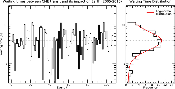
By comparing the catalog of the 107 CME events with the list of the associated geomagnetic storms, it is possible to construct the waiting time distribution (WTD) between the CME transit and its impact on Earth, allowing the estimation of a mean delay between the warning and the geomagnetic effect, with some confidence interval. This is shown in the right panel of Figure 2, where it is fitted with a log-normal function (red curve).

Zoom In Zoom Out Reset image size

Since the WTD between CME and geomagnetic event timings is well reproduced by a log-normal distribution, it is possible to state that the most probable delay between the times of detection of the CME predicted to be geoeffective and the geomagnetic storm is 4 hr and that 98% of the delays lie in the 2–8 hr interval.

Obviously, the number of false positives, the procedure efficiency, and the confidence interval of the waiting times are functions of the thresholds of the MHD quantities used in the analysis. The lower (higher) the thresholds, the higher (lower) the efficiency, but also the larger (smaller) the number of false positives and the broader (narrower) the confidence interval. The predictive tool can therefore be iterated by tuning these thresholds (for instance, by considering different values for different intervals over the course of the solar cycle) in order to maximize its efficiency also for moderate geomagnetic storming (−50 nT > DST > −100 nT) and to provide more accurate predictions by reducing the confidence interval of the most probable waiting time between CME and geomagnetic events, however, taking care not to introduce false positive signals. However, this is devoted to a future work.

It is worth noting that the flux ropes identified in the present analysis have a solar origin, being transported by CMEs. They thus represent a particular class of flux ropes. These magnetic structures may indeed also form locally in the solar wind or may be the remnants of the streamer belt blobs formed from disconnection. The automated detection of small-scale flux ropes of both solar and local origin, based on the Grad–Shafranov (GS) reconstruction, has revealed the existence of much more frequent flux ropes in the solar wind, at an occurrence rate of a few tens per day (Hu et al. 2018; Zhao et al. 2018, 2019; Chen et al. 2019). The tool presented in the present paper can be thus potentially used to identify also those flux ropes forming in the interplanetary space and advected by the solar wind. In this context it will be extremely interesting to compare the flux rope databases obtained on the basis of the GS reconstruction and the magnetic helicity analysis.

A new tool for the forecasting of geoeffective CME events based on in situ solar wind data acquired at 1 au has been developed. The novelty of this predictive approach resides (i) in the possibility of properly localizing CME structures by measuring the magnetic helicity content carried by the flux ropes, which have been recently proved to universally be the core magnetic structure of CMEs, and (ii) in the capability of accurately ascertaining which CMEs are really effective at causing geomagnetic effects, by quantifying their energetic budget. Since it is expected that more intense levels of geomagnetic storming are favored when the energy content carried by CMEs is larger, this tool can potentially forecast not only the CME-driven geomagnetic storms, but also their intensity.

A test campaign performed on the 12 yr time interval from 2005 to 2016 shows that the tool predicts, with an efficiency of 86%, any geomagnetic disturbance registered in Earth-based magnetometers as a sudden decrease of the DST index below −50 nT, providing an advanced alert lying, with a 98% confidence level, between 2 and 8 hr. Although Vourlidas (2014) has provided evidence for the presence of magnetic flux ropes within any CME, the existence of CMEs not embedding flux ropes, and thus not characterized by a strong magnetic helicity state, cannot be fully excluded. The diagnostic algorithm would fail to identify these CMEs, which could therefore constitute a source of the inefficiency of the detection tool.

This new technique has been tested off-line on a historical Wind data set. Its capability in predicting geoeffective CMEs when used on real-time solar wind data, as those provided by the Deep Space Climate ObserVatoRy satellite, and, most importantly, its performances are to be yet fully investigated. Considerable efforts are currently being made in this direction by the Aerospace Logistics Technology Engineering Company engineering team, in order to test and optimize this code in real-time mode. Finally, it is worth noting that this novel tool could be even more powerful by exploiting in situ measurements of future solar sail missions, which will be placed at sub-L1 positions, approximately at 6 million kilometers from Earth (where the radiation pressure balances the Sun gravitational attraction), thus allowing a longer, real-time advanced warning of any Earth-directed CME.

This work was partially supported by the Italian Space Agency (ASI) under contract I/013/12/0. Wind data and geomagnetic indexes were downloaded from the NASA-CDAWeb⁴ and WDC-Kyoto⁵ websites, respectively.