


Abstract
We employ a flux transport model incorporating observed stellar activity relations to characterize stellar interplanetary fields on cycle timescales for a range of stellar activity defined by the Rossby number. This framework allows us to examine the asterospheric environments of exoplanetary systems and yields references against which exoplanetary observations can be compared. We examine several quantitative measures of star–exoplanet interaction: the ratio of open to total stellar magnetic flux, the location of the stellar Alfvén surface, and the strength of interplanetary magnetic field polarity inversions, all of which influence planetary magnetic environments. For simulations in the range of Rossby numbers considered (0.1–5 RoSun), we find that (1) the fraction of open magnetic flux available to interplanetary space increases with Rossby number, with a maximum of around 40% at stellar minimum for low-activity stars, while the open flux for very active stars (Ro ∼ 0.1–0.25 RoSun) is ∼1–5%; (2) the mean Alfvén surface radius, RA, varies between 0.7 and 1.3 RA,Sun and is larger for lower stellar activity; and (3) at high activity, the asterospheric current sheet becomes more complex with stronger inversions, possibly resulting in more frequent reconnection events (e.g., magnetic storms) at the planetary magnetosphere. The simulations presented here serve to bound a range of asterospheric magnetic environments within which we can characterize the conditions impacting any exoplanets present. We relate these results to several known exoplanets and discuss how they might be affected by changes in asterospheric magnetic field topologies.
Export citation and abstract BibTeX RIS
1. Introduction
Since the 1990s, advances in astronomical observation techniques have led to the discovery of nearly 4000 confirmed exoplanets orbiting stars other than the Sun (Brennan 2019), with statistical arguments leading to the conclusion that most stars in the sky host at least one planet (Schrijver & Sojka 2016). As exoplanet detection is becoming more commonplace, the study of these planets is evolving from a phase of basic discovery to one of more in-depth characterization. An important aspect of this characterization is an understanding of the potential planetary magnetic impact of stellar activity: namely, the space physics of exoplanetary systems.
Current observational constraints limit our detection of habitable-zone Earth-sized exoplanets of significant interest to questions of habitability to those found in close-in orbits around small, cool M stars (Santos & Faria 2018), although these restrictions are changing with observations from the recently launched TESS mission (Huang et al. 2018). Though certain of these Earth-sized exoplanets, such as Proxima Centauri b, Ross 128 b, and several of the TRAPPIST-1 planets, are thought to reside in the conventionally defined circumstellar habitable zone (CHZ; Ramirez 2018), the low surface temperatures of these M dwarf stars result in CHZs many times closer to the star than the Earth–Sun distance. For example, Proxima Centauri b and Ross 128 b both have orbital semimajor axes of only about 0.05 au (Anglada-Escudé et al. 2016; Bonfils et al. 2018), and all seven known TRAPPIST-1 planets orbit within about 0.062 au of the star (Grimm et al. 2018). Here we constrain the space physics implications of such systems via a treatment of the magnetic and energetic properties of inner asterospheres for a range of stellar magnetic activity.
Cool stars like the Sun typically support global magnetic fields that, in turn, lead to a range of long-term (cyclic) and transient (in the form of flares and coronal mass ejections) stellar activity. These fields are thought to be generated via a combination of rotation and convection processes deep within the stellar interior (Yadav et al. 2015). The role of stellar parameters such as size, age, and rotation is critical in understanding the underlying physics governing the observed magnetic activity. The dependence of magnetic activity on dynamo action has led a number of authors to characterize stellar activity by the Rossby number, Ro = Prot/τc, where Prot is the star's rotation period and τc is the convective rollover time (Noyes et al. 1984; Jordan & Montesinos 1991). We note that Rossby number is often derived from empirical fits to observations and not from dynamo first principles (Reiners et al. 2014); however, the stellar Rossby number has been found to describe well the activity–rotation relations of populations of both partially and fully convective stars, indicating that the Rossby number may act as a robust descriptor of activity across a broad range of stellar types (Wright et al. 2011).
Stellar activity is determined in part by stellar parameters such as rotation period, cycle period, and meridional flow speed. These parameters are interconnected through stellar activity relations determined from astronomical observations (Noyes et al. 1984; Wright et al. 2011; Reiners et al. 2014; Brun & Browning 2017):


where Pcyc is the stellar activity cycle period, Prot is the equatorial stellar rotation period (24 days for the Sun), ϕ is the average magnetic flux over the stellar surface, Ro is the Rossby number, R* is the stellar radius, and vme is the meridional flow speed. We expand the observed behavior of the Sun to other stars (see Section 2) based on these empirical relations. We consider stars in the range from 0.1 to 5 times the solar Rossby number, RoSun. We scale to RoSun as there is some intrinsic uncertainty in our knowledge of this value (Reiners 2012). We use the above observed interrelationships to generate internally self-consistent simulations of the emergence of stellar flux and its evolution over time for a wide range of stellar activity, extending the application of previous solar flux transport modeling efforts (e.g., Schrijver et al. 2003).
The flux transport model employed here is derived from flux emergence patterns and flow behaviors observed on the Sun over almost a full magnetic cycle (see Section 2 for model description). Since there is much uncertainty in and very few direct or spatially resolved observations of flux emergence and evolution for stars other than the Sun, we do not attempt to simulate the surface magnetic distributions of any specific exoplanet host star. Moreover, much work is required to fully understand the flux emergence processes on stars of different stellar types than the Sun; this scientific question will form the basis of future investigations (see Section 4). For the present, we assume that the dynamical evolution of surface flux in most cool stars exhibits similar behavior when relevant rotation and meridional flow rates are taken into account (Wright et al. 2011). Stars with Rossby numbers greater than about 0.1 display an empirical inverse relation between Rossby number and stellar activity measures such as magnetic field strength and coronal emission; this "unsaturated regime" of the Rossby number–activity relation applies to a wide range of stellar types including M and G dwarfs (Wright et al. 2011). With respect to the evolution of flux distributions that result from the emergence process, evidence from full dynamo calculations suggests similarities in the surface flows and cycle variability of convective envelope stars like the Sun and fully convective M stars (Yadav et al. 2015). The Wright et al. (2011) observations and the modeling results of Yadav et al. (2015) lend confidence to our modeling framework's ability to capture the basic trends of stellar magnetic field evolution with activity. Therefore, in the absence of direct stellar evidence to the contrary, and in consideration of the dynamo arguments for comparable magnetic flux evolution behavior across stellar types, we assume solar flux emergence profiles (Equation (4)) for each star considered and concentrate on the trends implied by the changing levels of stellar activity.
In this work, we are motivated to consider how knowledge of the Sun–Earth system can be extended to characterize the impact of magnetic and energetic stellar activity on exoplanets, following on from previous investigations (e.g., Cohen et al. 2011). As a complement to the available observations of exoplanet host stars, which often lack significant temporal coverage and spatial resolution, we simulate stellar photospheric and coronal magnetic field distributions over stellar cycle timescales. The effect of this stellar magnetic activity on associated exoplanets is potentially a major factor in the broader question of planetary habitability.
In Section 2 we describe the flux transport model, its scaling to stars of greater or lesser activity than the Sun, and the properties of large-scale stellar magnetic fields over stellar cycle timescales. We present our analysis of these simulations, showing some of the relevant magnetic quantities, in Section 3, and we conclude in Section 4.
2. Simulating the Asterospheric Magnetic Field over Time
Magnetic field behavior in stellar atmospheres and beyond into interplanetary space is rooted in and driven by magnetic flux concentrations emerging through and evolving at the stellar photospheres. An understanding of the space environment in planetary systems must be built on detailed knowledge of the behavior of the magnetic field of the star. To this end, we employ a solar magnetic flux transport model developed by Schrijver and colleagues (Schrijver 2001; Schrijver & Title 2001; Schrijver et al. 2003) to treat the emergence, evolution, and dissipation of stellar magnetic flux self-consistently across a range of stellar activity. The bipolar magnetic flux emergence profile takes into account the relationship between active and ephemeral regions (Hagenaar et al. 1999) and is given by

where α = 1/3 represents the relative components of the flux in active and ephemeral regions, as observed on the Sun; a0 = a1 = 8 and p = 1.9 represent the active region flux spectrum observed at solar maximum; S is the area of the emerging bipoles in deg2; and  is the flux injection multiplier parameter (ϕ*/ϕ⊙) that we vary to simulate stars of different flux strength in accordance with Equation (2). The time variability of
  over the course of a stellar cycle is given by Equation (2) of Schrijver & Title (2001).
This surface flux transport (SFT) model employs a full 22 yr magnetic cycle of solar observations to parameterize the behavior and variation over time of the solar photospheric magnetic flux. The model operates by keeping track of the positions and fluxes of tens of thousands of fiducial flux concentrations that, in sum, represent the solar photospheric flux while using empirical prescriptions for flux emergence, advection, dispersal, and removal. The addition of flux to the model is based on the observed distribution functions of bipolar flux emergence across a broad range of size scales, ranging from the largest active regions to the smaller ephemeral regions, all of which have been well studied on the Sun. The distributions used in the SFT model are taken from Harvey & Zwaan (1993) and Hagenaar et al. (2003) for flux pairs on the larger and smaller ends of the spectrum, respectively, and are a function of activity cycle phase, latitude, and size.
Once flux has emerged onto the solar photosphere, most of the flux is observed to be passively advected by the large-scale zonal and meridional flows on the Sun. In the SFT model, an empirical rotation rate is used (see Snodgrass & Ulrich 1990; Komm et al. 1993) that applies to magnetic features of all sizes. The modeled differential rotation rate Ω is a function of latitude θ as follows:

where  deg day−1. The a coefficient is near zero because the model operates in a frame rotating close to the mean stellar rotation rate. The differential rotation multiplier d is a controllable parameter in the SFT model but is not modified for the simulations presented in this work (see Table 1).
Table 1. SFT Model Input Parameters for the Simulations Presented in This Study
| Ro/RoSun |

|
veq (km s−1) | Pcyc (yr) |

|
d (Equation (5)) |
|---|---|---|---|---|---|
| 0.1 | 31.6 | 20 | 2.19 | 12.9 | 1 |
| 0.25 | 8 | 8 | 5.475 | 4.666 | 1 |
| 0.5 | 2.83 | 4 | 10.95 | 2.16 | 1 |
| 0.75 | 1.54 | 2.667 | 16.425 | 1.377 | 1 |
| 1 | 1 | 2 | 21.9 | 1 | 1 |
| 2 | 0.354 | 1 | 43.8 | 0.463 | 1 |
| 3 | 0.19 | 0.67 | 65.7 | 0.295 | 1 |
| 4 | 0.125 | 0.5 | 87.6 | 0.214 | 1 |
| 5 | 0.089 | 0.4 | 109.5 | 0.167 | 1 |
Note. Each row represents a simulated stellar photosphere with the stated Rossby number Ro and the corresponding input parameter values. The SFT model parameters include the flux emergence strength  , stellar equatorial rotation speed veq, stellar magnetic cycle period Pcyc, meridional flow multiplier m, and differential rotation multiplier d. The input parameter values were chosen using Equations (1)–(3).
Download table as: ASCIITypeset image
The poleward meridional flow M(θ) is characterized by

in units of m s−1, taken from the correlation study of Komm et al. (1993). The meridional multiplier m is defined in this work in accordance with the meridional flow speed relation given in Equation (3). Both the differential rotation and meridional flow profiles are symmetric across the equator and do not evolve with time.
In addition to transport by the large-scale flow fields, convective flows present on the Sun affect the evolution of solar flux. This process is modeled in the SFT in a random-walk-like manner, with the displacement of stronger flux elements observed to be smaller than that of weaker flux elements. This coupling reflects the feedback that more concentrated fluxes, such as those within active regions, have on the flows in which they are embedded. These trends were demonstrated in Schrijver et al. (1996) and Hagenaar et al. (1999). Flux concentrations on the Sun are also observed to both spontaneously fragment and collide with neighboring flux concentrations (Schrijver et al. 1997); these processes are implemented in the SFT model.
Taken together, these empirical prescriptions comprise an SFT model that reproduces remarkably well the long-term patterns of flux evolution on the Sun. For example, Schrijver (2001) showed that this model mimics the character of observed solar magnetograms and flux density histograms. Additionally, applications to more active stars have successfully reproduced features such as polar spots (Schrijver & Title 2001) and X-ray/magnetic field flux–flux relations (Schrijver et al. 2003; Schrijver & Title 2005), providing evidence to support the application of the solar-derived SFT to other stars.
We apply this SFT model across a range of stellar activity in order to represent and examine the asterospheric environments of a variety of potential exoplanet host stars. Variation of the model's empirical-based activity parameters allows us to explore a wide range of "modified Suns." Stellar activity relations (1)–(3) constrain the parameter choice to a self-consistent set of values defined by the star's Rossby number (see Table 1). We use these activity relations to explore the asterospheric magnetic environments of these simulated stars for a range of plausible stellar activity levels. This approach is an extension of past applications of the model in that we have here included observationally motivated variations in meridional advection and stellar cycle periods.
Current observations of stellar magnetic fields are limited in spatial resolution and temporal coverage. Zeeman Doppler imaging (ZDI) techniques provide rudimentary estimates of the large-scale dipole component of the star's magnetic field (Reiners & Basri 2006) that can occasionally be extended to some characterization of the multipolar contribution (e.g., Lehmann et al. 2018). However, ZDI techniques may significantly underestimate stellar field strengths if one or more Stokes parameters are undetectable (Rosén et al. 2015). The ability to simulate the detailed behavior of stellar magnetic fields over a range of flux, spatial, and temporal scales allows us to explore a range of potential planetary impacts and lay the groundwork for direct comparison with current and future observations.
A great advantage in using the SFT is the highly tunable range of parameters controlling the emergence of magnetic flux and its behavior in time. Stellar activity in the form of magnetic field concentration in starspots, as well as flaring associated with these regions, is highly correlated with the rotation speed of the star and the meridional (poleward) flows of the magnetic flux (Brun & Browning 2017; Imada & Fujiyama 2018; Lehmann et al. 2018). Using SFT as a laboratory in which to study these stars, we are able to vary the rate of flux emergence, rotation rate, meridional flows, and other inputs to match observed stellar parameters and, in particular, their interrelationships. Additionally, our approach has an advantage over computationally expensive full dynamo simulations (e.g., Lemerle et al. 2015; Yadav et al. 2015), since it evolves magnetic flux concentrations at the stellar surface only and does not incorporate the complex and often poorly constrained internal behavior of the stellar dynamo.
In order to address the large-scale asterospheric field, we employ a field extrapolation approach, known as the potential field source surface (PFSS) method, commonly used in solar studies (Schatten et al. 1969). The PFSS approach calculates a current-free three-dimensional magnetic field distribution in the region above the photosphere, extending to a boundary, the source surface, at which the field is forced to become strictly radial. This condition serves to mimic the observed phenomenon that the solar wind becomes largely radially directed at several solar radii from the solar surface. In the solar case, such potential field models have been found to compare favorably with more sophisticated magnetohydrodynamic (MHD) solutions of field connectivity (Riley et al. 2006), though there is some debate as to whether the PFSS method fully captures the dynamics of the stellar wind plasma flow. For instance, Cohen (2015) found that PFSS treatment of the stellar atmosphere is largely unsuitable for estimating the speed and structure of stellar wind plasma flows. While the stellar wind plasma behavior is an important factor in the stellar impact on exoplanets, this work focuses strictly on the large-scale interplanetary magnetic field and its behavior with stellar activity. Within the solar community, the PFSS model is generally regarded as a sufficient measure of the large-scale magnetic field connectivity (e.g., open field versus closed field; Wallace et al. 2019).
Here we employ the PFSS method, as it provides an idealized but useful picture of the large-scale magnetic connectivity of the stellar atmosphere, as well as the magnetic field distribution that facilitates the propagation of the stellar wind into the inner asterosphere. A spherical source surface located at 2.5RSun is typically assumed for the solar case, although there is some suggestion that the location of this surface should be dependent on the strength of the surface flux and therefore vary with solar cycle (Lee et al. 2011). For stars more active than the Sun (Ro/RoSun < 1), Schrijver et al. (2003) found that the location of the source surface was proportional to the average flux, rising from 2.5 to 19 Rstar as the activity increases from solar to 10 times solar. To date, there has been no study considering the optimal distance of the source surface for high Rossby number stars. However, it is reasonable to assume that a source surface distance comparable to that of the Sun is required to adequately represent the coronal field as it transitions from a field- to a wind-dominated flow. We therefore adopt a minimum source surface radius of 2.5 Rstar for simulations with Ro/RoSun > 1 and use the Schrijver et al. (2003) scaling for high-activity stars. This approach of allowing the source surface to scale with stellar magnetic field strength mitigates the error possibly introduced when applying PFSS with the standard source surface radius 2.5 Rstar to a range of stellar activity levels.
In combining the stellar SFT simulations with potential field coronal extrapolations, we obtain a set of self-consistent three-dimensional magnetic field distributions extending from the stellar surface into the corona and inner asterosphere. These models have finely gridded spatial magnetic fields, as well as complete temporal coverage as the field distributions evolve over several stellar cycles. Thus, we have constructed a set of virtual asterospheres, differentiated by their surface flux and related magnetic activity, that can be examined for their potential impacts on associated exoplanets. Figure 1 displays the results of a solar test case simulation, as well as those for a more active (Ro = 0.5 RoSun) and a less active (Ro = 4 RoSun) star. Both the line-of-sight magnetograms of the simulated photospheres and the coronal magnetic field line distributions are displayed at stellar cycle maximum for direct comparison.

Figure 1. Three example stellar flux transport simulations with associated coronal field extrapolations. Panels (a)–(c) display the stellar photosphere flux distributions for Ro = 0.5 RoSun, RoSun, and 4 RoSun, respectively. These flux distributions are represented in the form of line-of-sight magnetograms with white corresponding to positive magnetic polarity and black corresponding to negative magnetic polarity. Panels (d)–(f) display the associated coronal magnetic field line distributions for each stellar simulation, extrapolated using the PFSS method. Field lines in magenta (outward) and green (inward) represent fields that cross the source surface and extend into interplanetary space, forming the magnetic field of the inner asterosphere. Field lines depicted in black represent closed magnetic field lines with each end rooted in the stellar photosphere, forming the loop structures of the stellar corona.
Download figure:
Standard image High-resolution imageFigures 1(b) and (e) show the solar simulation at cycle maximum. The more active stellar simulation, again at cycle maximum (Figures 1(a) and (d)), contains many more strong and complex magnetic flux concentrations, as well as enhanced magnetic flux in the quiescent regions outside of the starspots. Figures 1(c) and (f), representing cycle maximum for a less active star, have fewer large active regions but still contain a global distribution of small-scale ephemeral regions. The clear increase of magnetic complexity with decreasing Rossby number is also evident in the coronal field distributions. The strength and complexity of the stellar magnetic field has implications for the exoplanet environment: the effect of a star on a planet is largely governed by the nature of the global stellar magnetic field, its related dynamical behavior, and its evolution over time.
We examine a set of Rossby numbers in the unsaturated regime of stellar activity. Observations of cool stars have shown that for Rossby numbers in the range from about 0.1 to 10, stellar activity—chiefly in the form of indicators such as X-ray luminosity, chromospheric emission, or average magnetic field strength—declines steadily with increasing Rossby number, scaling approximately logarithmically (e.g., Reiners et al. 2014; Wright & Drake 2016). For smaller Rossby numbers, Ro < 0.1, observations show that stellar activity becomes effectively independent of Rossby number, and the activity "saturates." Stellar observations have shown the dichotomy between the saturated and unsaturated regimes to be robust for populations of partially convective cool stars like the Sun, as well as for fully convective stars like Proxima Centauri (Wright et al. 2011; Wright & Drake 2016). We restrict the application of the SFT model to stars in the unsaturated regime.
3. Characterizing the Asterospheric Fields of Exoplanet Host Stars
The SFT model, coupled to the PFSS extrapolation, allows us to characterize the coronal and asterospheric magnetic fields of active stars as a function of stellar activity via the Rossby number and the relationships defined in Equations (1)–(3). The topology and strength of the asterospheric field are key to understanding the magnetic and energetic environment in which exoplanets reside. Here we introduce and investigate several quantitative measures of star–exoplanet interaction: the ratio of magnetic flux open to the asterosphere, the location of the stellar Alfvén radius, and the strength of magnetic polarity inversion crossings for planetary orbits.
3.1. Stellar Magnetic Field Topology
Figure 2(a) displays the variation of the fraction of magnetic flux contained in open-field lines relative to total stellar flux as a function of Rossby number. This quantity is analogous to the asterospheric flux defined in Schrijver et al. (2003), except that (a) here we scale the open flux to the star's total flux for direct comparison across a wide range of stellar activity, and (b) we have included the variation of surface flows and stellar cycle parameters in the stellar models in accordance with the observationally motivated relations of Equations (1)–(3). Additionally, this quantity reflects the complexity of the stellar magnetic field topology, with more complex fields containing lower fractions of open magnetic field lines; this magnetic field complexity has been studied for others stars, such as young, fast rotators in open clusters (Garraffo et al. 2018). In particular, Garraffo et al. (2018) found that the evolution of rotation rate in young stars depends strongly on magnetic complexity, as some fast-rotating stars transport angular momentum less efficiently to the stellar wind and thus have persistent fast rotation rates. While we limit our focus to stellar cycle timescales, where the Rossby number is constant for a given star, rather than the megayear-to-gigayear timescales on which stellar rotation period evolves, an understanding of the longer-term effects of magnetic complexity on stellar activity and its implications for the evolution of the magnetic environments of exoplanets is an important consideration in determining the current state of the planet. Exploration of the relation between stellar evolution with age and exoplanetary magnetic environment will form the basis of future work in this area.
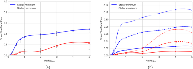
Figure 2. (a) Ratio of open-field flux to total surface magnetic flux as a function of stellar activity at stellar maximum and stellar minimum. Error bars are associated with a ±10% variation in the simulation source strength, corresponding to variation in the open to total flux ratio for a given Rossby number, Ro. (b) Ratio of open-field flux to total stellar flux in three latitude bands: ±0°−30° (solid lines), ±30°–60° (dashed lines), and ±60°−90° (dotted lines). Each data point represents an average of the quantity over the northern and southern hemispheres.
Download figure:
Standard image High-resolution imageThe SFT simulation results presented in Figure 2 are consistent with the observational trend of the logarithmic variation with Rossby number: all stellar simulations show more open flux at stellar minimum than at maximum as a result of the dominant dipolar nature of the minimum field. As the star approaches star-spot maximum, quadrupolar and higher-order components of the magnetic field grow, thereby contributing comparatively less magnetic flux that is open to the interplanetary medium (Wright & Drake 2016). Figure 2(a) also shows that stars more active than the Sun exhibit less variation in the proportion of open flux over the course of an activity cycle, since these very active stars will have complex and predominantly closed magnetic fields even at stellar minimum. Conversely, lower-activity stars have dominant dipolar magnetic fields with a more open field, principally at the stellar poles (see also Figure 1).
It is also useful to consider the variation of open field with latitude as a function of stellar activity; we can examine the open flux in the bands within 30° north or south of the stellar equator as a measure of the available flux in low-latitude regions of the asterosphere. Figure 2(b) demonstrates that the fraction of open flux at low latitudes (solid lines) does not vary significantly with activity, although there is a clear separation between stellar maximum and stellar minimum. It is clear that the open flux is predominantly defined by the high-latitude field (e.g., polar coronal holes) and that the fraction of open flux at high latitudes increases dramatically with decreasing activity (see Figure 1 (f) and Reiners & Basri 2006). The low latitudes (±0°−30°; solid lines) show the least variability, which is expected, as the equatorial activity belt is typically composed of closed-field active regions for all activity levels. The largest variation in the asterospheric field topology with activity is associated with the higher-latitude bands (dashed and dotted trend lines, respectively, in Figure 2(b)), particularly for stellar maximum (red). At low Rossby numbers, the stars are very active and likely dominated by a disordered, closed field, even at stellar minimum, when the dipole component of the field is expected to be relatively strong. This effect is even more pronounced at stellar maximum (see, for example, Figure 1(d)), when the open flux ratio rises sharply for a high Rossby number because stellar maximum is still dominated by the overall dipole component.
We consider the variation of open-field magnetic flux as an indicator of the availability of the magnetic field to the asterosphere and the stellar wind. The closed magnetic field structures that make up the stellar atmosphere also play a significant role in stellar activity with substantial planetary impact; the production of energetic EUV and X-ray emission in closed coronal field structures has implications for planetary magnetosphere energization, variations in ionospheric conductance, atmospheric chemistry, and atmospheric loss (Airapetian et al. 2017). Hydrostatic and hydrodynamic models of stellar coronal heating provide a means to relate the simulated flux distributions and their associated 3D closed-field structures to the expected energetic plasma emission. Such simulations provide self-consistent stellar X-ray and extreme ultraviolet (XUV) emission outputs that subsequently serve as inputs to associated planetary magnetospheric and ionospheric modeling, as well as providing opportunities for direct comparison with stellar observations (A. O. Farrish et al. 2019, in preparation; A. M. Sciola et al. 2019, in preparation).
3.2. Alfvén Surface
An important consideration in examining the magnetic interactions between a star and a planet is the location of the planetary orbit relative to the stellar Alfvén surface. We define the Alfvén radius as the average radius around a star at which the stellar wind energy density equals the asterospheric magnetic field energy density. At the radial distance of the Alfvén surface, RA, the stellar wind transitions from sub- to super-Alfvénic. A planet orbiting periodically or continually inside this surface may be directly magnetically connected to the stellar corona, with potentially disastrous effects on atmospheric retention (Garraffo et al. 2017); a planet with an orbit placed well outside this boundary will be decoupled from the coronal magnetic field and will interact with the stellar wind in a manner similar to that of the Earth.
Depending upon the assumptions one makes about the nature of the stellar wind (e.g., thermally or turbulently driven), the Alfvén boundary may not be purely spherical but rather have a convoluted shape that depends strongly on photospheric magnetic field distributions and the variation of the Alfvén speed in the stellar corona (Scherer et al. 2001). Previous modeling efforts have demonstrated, for example, that the extent of the Alfvén surface may be smaller at the equator and larger at the poles for a star of a given activity level and rotation rate (Réville et al. 2015). We restrict our considerations here to a spherical Alfvén surface as a representative measure of the transition to a stellar wind-dominated magnetic field, enabling us to consider large-scale changes as a function of stellar activity and stellar cycle phase without recourse to a highly parameterized and computationally expensive wind model. We extend previous Alfvén surface analyses to consider a range of potential host star activity and the associated effect on the Alfvén surface, based on the spatially averaged magnetic flux of the star. While the exact extent of atmospheric erosion due to a direct magnetic connection to the stellar corona is not within the scope of this work, it is certain that a planet orbit embedded continually or periodically within its host star's Alfvén surface would reside in a significantly more hostile space weather environment than that of the Earth.
Following Schrijver et al. (2003), we employ a scaling law for the calculation of the Alfvén radius, RA, under the assumption of a thermally driven stellar wind,

where ϕ* is the average magnetic flux at the stellar surface. This relationship is derived from a detailed consideration of angular momentum loss via the stellar wind while also including the simplifying assumption that the Alfvén speed vA is equal to the stellar wind speed at large distances from the stellar surface  . We scale these values to the analogous values for the Sun at solar maximum. It is estimated that the solar Alfvén surface has an average radius of ∼20 RSun (≈0.1 au) at solar maximum (Chhiber et al. 2019).
Figure 3(a) presents the Alfvén radii we find at both stellar minimum and maximum phases for our chosen range of stellar activity. Also shown in Figure 3(b) are the locations (planetary orbit semimajor axis versus host star Rossby number) of several known exoplanets where we assume a fiducial solar Alfvén radius of 20 RSun and a solar Rossby number of 1.85 (Stepien 1994, consistent with Wright et al. 2011). We see that the orbits of some widely studied habitable-zone planets—Proxima Centauri b, Ross 128 b, and TRAPPIST-1 c, e, g, and h—all reside well within the Alfvén surfaces of their host stars at all times over the stellar cycle. Of the two planets within the GJ 3323 system (Astudillo-Defru et al. 2017), GJ 3323 b lies well within the Alfvén radius, while GJ 3323 c skirts the Alfvén surface at stellar minimum. Different models of the stellar wind or the assumption of a larger solar Alfvén radius could result in GJ 3323 c also falling within this crucial surface, significantly affecting its physical state. The points representing Ross 128 b and the recently discovered planets around Teegarden's star (Zechmeister et al. 2019) were generated by estimating the Rossby number of their respective stars using Equation (11) in Wright et al. (2011) to determine the convective rollover time from the stellar mass and an assumed rotation period of ≈100 days, reflecting the expectation for low-mass stars (<0.1 MSun) with no significant Hα emission (see Bonfils et al. 2018 and Newton et al. 2017). The error in the Rossby number is likely to be high. We scale to the assumed value RoSun = 1.85 in each case (Wright et al. 2011).
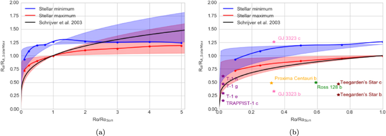
Figure 3. (a) Alfvén surface radius as a function of stellar activity at both stellar minimum and stellar maximum. The Alfvén radius is scaled to the value for the Sun at solar maximum, equal to ∼20 RSun. Shaded error regions are associated with the uncertainty in the exponent of Equation (4). For comparison, we show the relationship derived via Schrijver et al. (2003). (b) The orbital locations of several known close-in exoplanets are shown in relation to observational estimates of their host stars' Rossby numbers. Many known exoplanets with orbits on the order of 1 au or farther lie far above the upper limit of the plot and are not expected to interact measurably with the host star's Alfvén surface.
Download figure:
Standard image High-resolution imageThese results compare well with previous modeling efforts incorporating a more detailed MHD stellar wind that demonstrated, for example, that Proxima Centauri b might cross in and out of its star's Alfvén surface over the course of each 11 day planetary orbit (Cohen et al. 2014); see also similar arguments for the TRAPPIST-1 planets (Garraffo et al. 2017). In the simulations presented here, we have assumed a thermally driven wind expressed by a constant  ; a turbulently driven wind results in a radial and latitudinal variation in the local Alfvén speed (Cohen et al. 2014; Garraffo et al. 2017), resulting in a more structured Alfvén surface.
Figure 3(b) implies that, however the Alfvén surface is defined, many of the Earth-sized planets of interest for possible habitability reside inside or near the Alfvén surface boundary of their small, cool host stars and therefore experience vastly different magnetic environments than that of Earth. Our results are important to long-term prospects for habitability in these and other systems of extreme star–planet proximity, since the location of these planets relative to their stars is almost certainly an unfavorable configuration for a hospitable space weather environment or, at the very least, an extremely exotic system compared to that of Earth and the Sun.
3.3. Stellar Wind Magnetic Polarity Inversions
Finally, we consider the complex structure of the interplanetary magnetic field and its potential for creating magnetic activity at the planet. The asterospheric current sheet (ACS; Wilcox et al. 1980) defines the boundary between opposite polarities in the large-scale stellar magnetic field; a simple stellar dipole field (e.g., Figure 1(f)) leads to an unstructured ACS centered on the stellar equator (see Figure 4(f)). Naturally, a more active star, or a star at a more active phase of its cycle, has higher-order components in its global magnetic field, particularly in the low-latitude activity belt, and the ACS becomes more complex with significant excursions (Lundstedt et al. 1981; Nayar & Revathy 1982). Figure 4 shows the radial magnetic field at the stellar source surface for each of the activity levels presented in Figure 1 (Ro/RoSun = [0.5, 1.0, 4.0]). The increase in complexity is obvious as the activity level increases. Solar maximum activity (Figure 4(b)) shows a highly structured ACS with major poleward excursions in both hemispheres. High-activity, low Rossby number stars have a far more complex and disorganized structure (Figure 4(a)) and even experience significant deviations from dipolar magnetic structure at the minimum activity phase (Figure 4(d)).
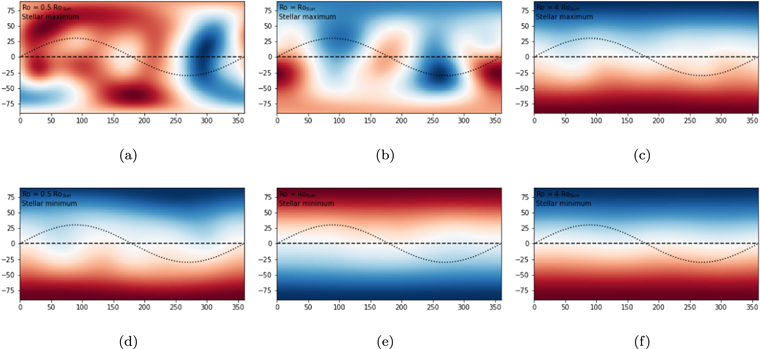
Figure 4. Radial magnetic field component Br at the source surface for the same simulations shown in Figure 1 (Ro/RoSun = [0.5, 1.0, 4.0]), shown at both stellar minimum (bottom) and stellar maximum (top). The projection of two theoretical planetary orbits with 0° (dashed) and 30° (dotted) inclinations are shown.
Download figure:
Standard image High-resolution imageAlso shown in each panel of Figure 4 are projected orbits for two hypothetical planets with inclination angles to the stellar equator of 0° and 30°. The potential for significant planetary magnetic activity resulting from increased stellar magnetic complexity has been extensively studied for the Sun with a number of case and statistical studies emphasizing the importance of sector boundary crossings (SBCs) for driving geomagnetic activity; SBCs signify sharp transitions in the sign of the stellar radial field. It has been shown (Asenovski 2017) for the solar case that sector crossings (radial magnetic field directed away/toward or toward/away from the Sun) are frequently associated with moderate to strong geomagnetic storms. Further, Khabarova & Zastenker (2011) demonstrated that the rapidity of the transition between magnetic polarities is also an important feature in driving strong magnetic activity at the planet. Additionally, a comprehensive statistical analysis of the impact of solar magnetic structures on geomagnetic activity by Echer & Gonzalez (2004) has shown that SBCs alone are moderately geoeffective (∼26% of SBCs leading to moderate to intense activity) but have an increased impact when they are associated with other interplanetary magnetic structures such as magnetic clouds and corotating streams: 100% of magnetic clouds at or near SBCs were found to be geoeffective (compared to 77% of magnetic clouds as a whole). The strength of any planetary magnetic activity resulting from stellar magnetic complexity is dependent on a number of factors: the presence of SBCs, high-speed streams, and magnetic clouds, as well as the strength and orientation of the planetary magnetic field. To fully constrain all of these factors would require detailed modeling coupled, ideally, with high-resolution observations of a particular star–planet pairing. In this paper, we use the variation in the SBC structure with stellar activity as a diagnostic for the potential for enhanced planetary magnetic activity and a consideration for future possible observational searches for associated planetary emissions.
In Figure 5(a), we show the behavior with stellar activity of the magnetic field gradient averaged over all SBCs experienced by the hypothetical planetary orbit of 0° inclination shown in Figure 4. Here we assume that the ecliptic plane coincides with the equatorial plane of the star. While the number of ACS SBCs is a good representation of the magnetic complexity of the inner asterosphere, the significant variability in the structure of the ACS over a stellar cycle limits the utility of this number as a definitive measure of strong planetary magnetic activity. However, it has been shown for the Sun that the steepness of the transition from one polarity to the other has a significant bearing on the intensity of the planetary magnetic response (Khabarova & Zastenker 2011). As such, we have adopted the average spatial gradient of the radial magnetic field across polarity inversions (either away/toward or toward/away) as a discriminator of potential planetary magnetic impact. Figure 5(a) shows that there is likely to be a substantial increase in the magnetospheric activity at the planet with increasing stellar activity/complexity. For stars significantly less active than the Sun (Ro/RoSun ≥ 2), there is very little variation in the structure and complexity of the ACS, and therefore the average strength of the polarity inversion crossings is comparatively low and exhibits little variation with Rossby number. Conversely, the trend shown in Figure 5(a) demonstrates that the typical crossing strength across boundaries between different magnetic polarities rises sharply with higher stellar activity. For all activity levels modeled, there is a clear distinction between stellar minimum and stellar maximum, with the latter showing significantly stronger gradients due to the stronger fields present at stellar maximum.

Figure 5. (a) Red and blue lines show the magnitude of the average radial magnetic field gradient at locations where the 0° inclination orbit (see Figure 4) traverses a polarity inversion crossing for stellar maximum and minimum, respectively. The values are normalized to the largest value in the set, the gradient at stellar maximum for Ro = 0.1 RoSun. (b) Red and blue lines show the magnitude of the average radial magnetic field gradient at locations where the 30° inclination orbit crosses a polarity inversion for stellar maximum and minimum, respectively. The values are normalized to the largest value in the set, the gradient at stellar maximum for Ro=0.1 RoSun.
Download figure:
Standard image High-resolution image
To place the possible impact of SBCs in the exoplanetary context, we must consider the relative timescales of the planetary orbital period and stellar rotation. The evolutionary timescale of the stellar magnetic field itself may also need to be taken into account, particularly when considering planets with long orbital periods or when the orbital and stellar rotation periods are comparable—in this case, the magnetic structure "seen" by the planet over time is more dependent on the changing surface field than on the planet's location in its orbit. Here we are interested in planets that are in close proximity to the star, where the potential for magnetic interactions is stronger; thus, we disregard the stellar field evolution timescale as being long compared to planetary orbit timescales (on the order of 5–10 days for most of the planets displayed in Figure 3(b)). We consider two cases: (a) a fast-rotating star with a planet of reasonably long orbital period and (b) a slow-rotating star with a close-in planetary orbit. In the former case, the planet can be regarded as effectively stationary as the asterospheric field sweeps past; in the latter case, the magnetic configuration can be assumed to be effectively stationary as the planet traverses the interplanetary magnetic structure (see the hypothetical orbital paths shown in Figure 4). For the zero-inclination orbit of Figure 5(a), these two scenarios are equivalent, and the planet effectively encounters the entire equatorial open-field structure, so that the planetary magnetic activity is driven, in part, by the SBCs encountered. For an inclined orbit, e.g., the 30° case considered, the situation is more complex. For case (a)—fast rotator, long-period orbit—the planet is effectively stationary at a specific asterographic latitude, depending upon where it is in its orbit, and the planet would experience any SBCs associated with that latitude. For case (b)—slow rotator, short-period orbit—the planet would sweep out a range of asterographic latitudes as shown in Figure 4, leading to a complex interaction with the ACS. In this case, a possible dominant signature in the average gradient would be the swing from the northern to southern hemisphere. This strong signature would appear at all activity levels and, as a result, the strength of SBCs would display only weak variation with activity.
In Figure 5(b), we show the results for a hypothetical planetary orbit with inclination 30° to the star's equatorial plane (assumed orthogonal to the star's rotation axis), following the sinusoidal curves displayed in the panels of Figure 4. Consistent with the reasoning above, there is little variation in the low-activity regime, where stellar rotation period is long compared to planetary orbital period, and the polarity inversions are dominated by a simple crossing of the magnetic equator. Unlike the 0° inclination orbit shown in Figure 5(a), there is no clear trend in the strength of polarity crossings at high stellar activity for the assumed 30° orbital inclination. This is due to the highly complex and disordered nature of the stellar magnetic fields at low Ro, complicated by the comparable timescales of stellar rotation and planetary orbit (low-Ro stars tend to be fast rotators). In the absence of real planetary orbits with independently defined inclinations and phases relative to stellar rotation, we must choose an arbitrary phasing of the orbit with respect to the magnetic structure, shown in Figure 4, and thus cannot draw universal conclusions from an arbitrary sampling of the stellar magnetic field polarity inversions for high stellar activity. For example, for the phasing selected in Figure 4(a), the planet traverses a large inversion in the radial magnetic field distribution at asterospheric longitudes of approximately 250° and 340°. A different choice of orbital phase might miss these large inversions and therefore change drastically the average strength of the planet's SBCs.
We consider these sharp transitions in the polarity of the stellar magnetic field because of the implications for strong and/or frequent opportunities for reconnection events in any planetary magnetosphere that may be present. The stronger the planetary magnetic response, the stronger its expected radio signature (Zarka 2010), thus placing important constraints on future exoplanetary observations.
A more complete picture of the potential asterospheric magnetic field effects on exoplanets will emerge as we broaden our investigation in future work to consider full MHD stellar wind calculations. This research will provide additional knowledge of the behavior of the stellar wind plasma and the kinetic (ρv2) energy density of exoplanet host stellar winds (S. Moschou et al. 2019, in preparation).
4. Discussion and Conclusions
Here we have presented a description of our methodology in applying solar physics modeling capabilities to questions of exoplanet host star behavior. We bridge the gap between heliophysics understanding of the Earth–Sun system and the open questions of characterizing star–exoplanet interactions. Combining a solar magnetic flux transport model with observed stellar physics relations and a global coronal field model, we are able to simulate the spatial and temporal variations of stellar magnetic activity for a range of possible exoplanet host stars. We have characterized the scaling using the Rossby number as a measure of stellar activity and magnetic field behavior for the unsaturated regime of the activity–rotation relation, which observational evidence suggests is robust for both solar-like partially convective stars and slowly rotating fully convective stars. This observational support for the scaling of the solar-based models to other stars is an encouraging result for this still-developing field of comparative heliophysics for exoplanet systems.
We note that these simulations do not represent the exact surface flux distributions of any given star, due to factors such as large uncertainties in measured stellar parameters, e.g., stellar cycles, rotation periods, and large- and small-scale magnetic field strengths. In addition, the current state of stellar observations provides very limited knowledge of the surface flows and internal dynamics of other stars, though advances in ZDI and asteroseismic observations may improve our understanding of these processes in the future (Reiners & Basri 2006). Rather than attempting an exact replication of the magnetic flux distribution and evolution on a particular star's surface, we instead consider a set of simulations that are representative of the levels of activity and the large-scale connectivity of asterospheric magnetic fields in general. We complement these simulated stellar photospheric magnetic field distributions by coupling to a potential field source surface model for the stellar corona and inner asterosphere; the PFSS extrapolations represent an ideal current-free magnetic field, a reliable descriptor of the large-scale connectivity and topology of the solar corona. Future work will incorporate more complex representations of the coronal field, such as MHD or force-free extrapolation methods, to discern contributions to star–planet interactions from nonpotential sources of coronal magnetic fields and currents.
We find that with increasing stellar activity, the fraction of magnetic flux topologically open to the stellar wind decreases as the coronal magnetic field increases in complexity, though it does become less restricted to the stellar poles; in addition, the variation across cycle timescales of this ratio decreases with decreasing Rossby number. One avenue of further investigation will be to combine this topological approach to wind structure with models of stellar wind speeds and pressures to provide a fuller picture of both the strength and spatial distributions of stellar winds affecting exoplanets (Scherer et al. 2001).
We also demonstrate via a flux-dependent scaling relation that the average radius of the stellar Alfvén surface decreases for small Rossby numbers but stays roughly constant at large Rossby numbers. We find that several close-in exoplanets around active host stars, e.g., Proxima Centauri b and the TRAPPIST-1 planets, reside entirely within their stars' Alfvén surfaces, effectively embedded in the potentially quite extreme environment of their host stars' coronae. With a more structured, turbulent-driven stellar wind, the interaction between the planets and their star's Alfvén surface may be more complicated (Garraffo et al. 2017). Investigation of the consequences for habitability of these planets is outside the scope of this work, but it is certain that such an environment would be very different than the magnetic environment at Earth. However, given the thermally driven wind assumption adopted here, GJ 3323 c would lie marginally outside the stellar Alfvén surface, having an orbital semimajor axis of 0.126 au; if the planet has a sufficiently strong magnetic field, it should be well protected from the stellar activity of GJ 3323 and an interesting target for future radio observations. For completeness, it is worth noting that GJ 3323 c also lies significantly outside the star's CHZ (estimated to be between 0.026 and 0.054 au) and outside Kopparapu's outer boundary for an early Mars (estimated to be 0.077 au; Kopparapu et al. 2013).
An important factor in the characterization of the physical nature of an exoplanet is the determination of its magnetospheric field. This requires modeling the planetary response to stellar activity. In the present work, we note that the increasing magnetic complexity associated with decreasing Ro is reflected in the number and intensity of the SBCs in the asterospheric magnetic field. While these characteristics of the ACS are by no means "fixed" for a given star at a given phase of its activity cycle, the modeling presented here does provide some insight into the exoplanet magnetic environments expected. This also provides useful contextual information for possible searches for exoplanetary radio signatures.
With the rapid growth in exoplanet discovery, there is a need for in-depth characterization of planetary environments, significant aspects of which are driven by interaction with their parent star. It is important to understand the physical conditions that underpin these interactions if we are to fully characterize planetary conditions, interpret observational signatures, help guide future searches, and refine our knowledge of the potential for habitability. Since present observational capabilities are not sufficient to detect key signatures that define the planetary environment, it is necessary to guide future observations by constraining the expected signatures via modeling and simulation. In this paper, we have considered the energetic interactions between stars and planets, their temporal evolution over stellar cycle timescales, and their expected impact on the magnetic environment of exoplanets. In future work, we will extend this analysis to the coronal XUV signatures associated with the stellar magnetic activity discussed here. Energetic XUV emission is an important component of the planetary response, as it drives ionospheric currents that serve to influence the planet's magnetospheric state.
We would like to acknowledge insightful discussion with Ofer Cohen as we were getting this project underway. This work was supported by an INSPIRE grant from the NASA Science Foundation (AST-1461918). Ms. Mei Maruo's participation was supported by the Tomodachi STEM @ Rice University Program funded by the US–Japan Council.