


Abstract
It is well established that solar flares and coronal mass ejections (CMEs) are powered by the free magnetic energy stored in volumetric electric currents in the corona, predominantly in active regions (ARs). Much effort has been made to search for eruption-related signatures from magnetic field observed mostly in the photosphere; and the signatures are further employed for predicting flares and CMEs. The parameters in the Space-weather HMI Active Region Patches (SHARP) data from the Solar Dynamics Observatory/HMI observation of vector magnetic field are designed and generated for this purpose. In this paper, we report research done on modification of these SHARP parameters with an attempt to improve flare prediction. The newly modified parameters are weighed heavily by magnetic polarity inversion lines (PIL) with high magnetic gradient, as suggested by Schrijver, by multiplying the parameters with a PIL mask. We demonstrate that the number of the parameters that can well discriminate erupted and nonerupted ARs increases significantly by a factor of two, in comparison with the original parameters. This improvement suggests that the high-gradient PILs are tightly related with solar eruption that agrees with previous studies. This also provides new data that possess potential to improve the machine-learning-based solar flare prediction models.
Export citation and abstract BibTeX RIS
1. Introduction
Solar flare prediction is one of the important topics in solar-physics and space-physics communities. Since released energy during flares mainly comes from the magnetic field in the corona, many studies have focused on searching for magnetic features and parameters that are related to solar eruption and on further establishing forecast schemes (see, e.g., Falconer et al. 2002; Leka & Barnes 2003, 2007; Barnes & Leka 2006, 2008; Cui et al. 2006; Jing et al. 2006; Georgoulis & Rust 2007; LaBonte et al. 2007; Schrijver 2007; Falconer et al. 2008; Bloomfield et al. 2012; Barnes et al. 2016). With quickly increasing interest in and success of pilot studies in the solar-physics community, machine-learning technology has opened a new window into the space weather forecast. Various models have been investigated and developed (e.g., Ahmed et al. 2013; Bobra & Couvidat 2015; Liu et al. 2017a, 2019; Nishizuka et al. 2017, 2018; Benvenuto et al. 2018; Florios et al. 2018; Huang et al. 2018; Jonas et al. 2018).
Specifications of observational data taken by the Helioseismic and Magnetic Imager (HMI; Scherrer et al. 2012; Schou et al. 2012) on board the Solar Dynamics Observatory (SDO; Pesnell et al. 2011), including full disk field of view, continuous observation coverage, high temporal and spatial resolutions, and consistent data quality, provide a unique opportunity to study solar eruption. The parameters in the HMI data product, the Space-weather HMI Active Region Patches (SHARP; Bobra et al. 2014), are specifically useful for searching for the relationship between magnetic properties in ARs and solar eruptions because these parameters, derived from the vector magnetic field, characterize magnetic field property, especially magnetic nonpotentiality, in ARs, and therefore contain magnetic signatures that are related to solar eruption (e.g., Leka & Barnes 2003; Bobra & Couvidat 2015). Indeed, these SHARP parameters have been widely used for predicting solar flares through various techniques and methods, including the machine-learning methods (see, e.g., Bobra & Couvidat 2015; Liu et al. 2017a; Florios et al. 2018; Inceoglu et al. 2018; Jonas et al. 2018; Chen et al. 2019), and some of the magnetic features have been shown to be effective in discriminating noneruptive and eruptive ARs and predicting solar flares (e.g., Bobra & Couvidat 2015; Liu et al. 2017a; Florios et al. 2018; Chen et al. 2019).
The magnetic polarity inversion line (PIL), the harbor to host filaments, has been shown to relate to solar flares and CMEs (e.g., Falconer et al. 2002; Schrijver 2007; Mason & Hoeksema 2010; Welsch et al. 2011; Georgoulis et al. 2012, 2019; Moore et al. 2012; Török et al. 2014; Liu et al. 2017b; Georgoulis 2018), indicating an area of interest in ARs that may contain a property of magnetic field configuration necessary for triggering and fueling solar flares. Schrijver (2007) analyzed 2500 ARs with MDI magnetograms (Scherrer et al. 1995) and concluded that "...large flares, without exception, are associated with pronounced high-gradient polarity-separation lines." In this study, we modify the SHARP parameters by multiplying with a high-gradient PIL mask before calculating the parameters. In this way, the resulting parameters are weighed heavily by the areas along the PILs. We evaluate the effectiveness of the newly modified parameters in discriminating the noneruptive and eruptive ARs. We conclude that the modified parameters are significantly better than the original ones at separating the two groups of ARs, and thus show great potential to improve the machine-learning-based solar flare prediction models.
The paper is organized as follows. In Section 2, we describe the data and the computation of the modified parameters. We present our results in Section 3. The conclusion is given in Section 4.
2. Data and Modified SHARP Parameters
2.1. Data
We use the SDO/HMI vector magnetic field data (Hoeksema et al. 2014) to produce the PIL mask and then calculate the parameters for the ARs. The HMI instrument is a filtergraph with full disk coverage at 4096 × 4096 pixels. The spatial resolution is about 1'' with a 0 5 pixel size. The spectral line is the Fei 6173 Å absorption line formed in the photosphere (Norton et al. 2006). The Stokes parameters [I, Q, U, V], measured at six wavelength positions and sampled every 720 seconds using a 1350 second weighted average, are inverted to retrieve the vector magnetic field using a Milne–Eddington based inversion algorithm, the Very Fast Inversion of the Stokes Vector (VFISV; Borrero et al. 2011; Centeno et al. 2014). The 180° degree ambiguity of the azimuth is resolved using a "minimum energy" algorithm (Metcalf 1994; Metcalf et al. 2006; Leka et al. 2009). The location and extent of the ARs are automatically identified and bounded by a feature recognition model (Turmon et al. 2010), and the disambiguated vector magnetic field data are deprojected to heliographic coordinates (Bobra et al. 2014). Here we use the Lambert (cylindrical equal area) projection method centered on the region for the remapping. The remapped data of the vector magnetic field in ARs is then used to compute the parameters.
We collect SHARP vector magnetic field data from 2010 May 1 to 2018 November 30 to form two data samples. One includes the data of eruptive ARs one hour before the major flares (M-class and above); the other includes the data of noneruptive ARs (one data point per day). Eruptive ARs are defined here as ARs that produced at least one major flare (M-class and above) during their disk passage; noneruptive ARs are those that do not produce any major flares during disk passage. The data of flares are obtained from the NOAA Space Weather Prediction Center. Only the ARs within 60° from the central meridian are selected. Following the above procedures, we have sampled a total of 313 data points for the eruptive ARs and 6633 data points for the noneruptive ARs. We use these two data samples for our study.
2.2. Modified SHARP Parameters
For the vector magnetic field data, we first use radial field, Br, to generate a PIL mask. We then multiply this mask with the SHARP parameter distribution maps derived from the vector magnetogram. Finally, we sum up all the pixels resulting in parameter maps to obtain the modified SHARP parameters.
The PIL mask is generated from Br using the method described in Schrijver (2007). We first produce two bitmaps from the Br map: one for positive field in which the pixels with Br > 200 G are set to 1 and the rest are 0; the other for negative field in which the pixels with Br < −200 G are −1 and the rest are 0. 200 G is about 2σ for HMI vector field data (Hoeksema et al. 2014). We then derive the positive and negative masks from the bitmaps using the Density-Based Spatial Clustering of Application with Noise (DBSCAN; Sander et al. 1998) method. We finally multiply the two masks after convolving with the masks a Gaussian kernel with a width of 10 pixels to generate the PIL mask. The SHARP parameter maps are calculated from the vector field data using the formulas listed in Table 1 that are modified from Table 3 in Bobra et al. (2014). The final modified SHARP parameters are then obtained after multiplying the parameter maps with the PIL mask. The modified SHARP parameters retain all the original ones except the parameters that are related with Lorentz force, because these parameters are global quantities (Fisher et al. 2012) which must be calculated using the data over all of the ARs. The parameters calculated from the area enclosed by the PIL mask only do not have physical meaning. As a result, the modified SHARP parameters include 16 physical quantities.
Table 1. Some of the SHARP Parameters, Modified from Table 3 in Bobra et al. (2014)
| Keyword | Description | Sharp Formula |
|---|---|---|
| TOTUSJH | Total unsigned current helicity |

|
| TOTPOT | Total photospheric magnetic free energy density |
|
| TOTUSJZ | Total unsigned vertical current |

|
| ABSNJZH | Absolute value of the net current helicity |

|
| SAVNCPP | Sum of the modulus of the net current per polarity |
|
| USFLUX | Total unsigned flux |

|
| MEANPOT | Mean photospheric magnetic free energy |
|
| R_VALUE | Sum of flux near polarity inversion line |
 within R mask within R mask |
| MEANSHR | Mean shear angle |
|
| MEANGAM | Mean angle of field from radial |

|
| MEANGBT | Mean gradient of total field |
|
| MEANGBZ | Mean gradient of vertical field |
|
| MEANGBH | Mean gradient of horizontal field |
|
| MEANJZH | Mean current helicity (Bz contribution) |

|
| MEANJZD | Mean vertical current density |

|
| MEANALP | Mean characteristic twist parameter, α |

|
Download table as: ASCIITypeset image
As an example, Figure 1 demonstrates the procedures to generate the PIL mask for AR 11158. The top left panel is Br taken at 01:12 UT, 2011 February 15. The top right and bottom left are bitmap masks for positive and negative fields, respectively. The PIL mask is shown in the bottom right panel. It can be clearly seen that the PIL is well characterized by the mask.
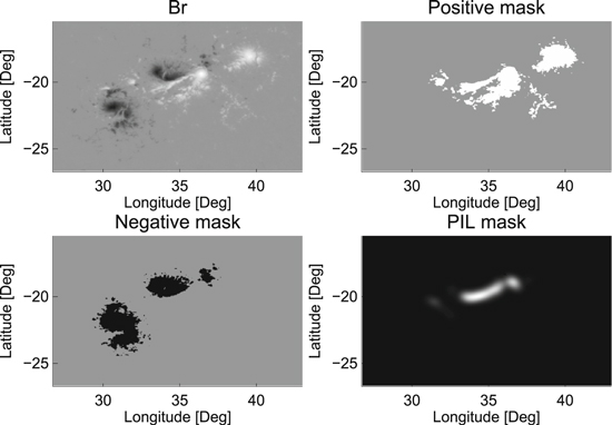
Figure 1. Top left: radial magnetic field, Br, in the active region AR 11158 taken at 01:12 UT, 2011 February 15. Top right: the mask of positive field derived from Br. Bottom left: the mask of negative field from Br. Bottom right: the PIL mask. See the context for details.
Download figure:
Standard image High-resolution imageFigure 2 shows the SHARP parameter maps for AR 11158. The panels in the first and third columns are the original parameter maps, while the second and fourth columns denote the modified maps multiplied with the PIL mask. In the modified maps, the parameters are excluded from most pixels in the images, except for the area enclosed by the PIL mask. The pixels finally chosen to calculate the modified SHARP parameters are indeed enclosed by the PIL mask, and also satisfy a high-confidence disambiguation threshold where the vector field has been disambiguated with high confidence (Bobra & Couvidat 2015). Thus, the modified SHARP parameters represent the physical quantities in the PIL areas.

Figure 2. Distributions of vector magnetic field and physical quantities for AR 11158 at 01:12 UT, 2011 February 15. The first and third columns refer to original data; the second and fourth columns show the original data multiplied with a PIL mask. Bh denotes the horizontal field. Btot denotes the total field. GAM denotes the angle of field from radial. SHR denotes the shear angle. Jz denotes the vertical current. DerivBz, DerivBh, and DerivBtot denote the gradients of radial, horizontal, and total fields, respectively.
Download figure:
Standard image High-resolution image3. Results
3.1. Discriminant Analysis
Figures 3 and 4 show distributions of the original and modified SHARP parameters, respectively. The black (red) curves refer to distributions of the parameters for the noneruptive (eruptive) AR sample. The two groups of data are described in Section 2.1. X-axis refers to the value of the parameters. The parameters are normalized. We use distributions of the total unsigned current helicity (TOTUSJH, top left panels) as an example to describe the plots. For both the original and modified TOTUSJH, most noneruptive ARs have low values and the peak of the distribution is thus on the low-value end (black); the value becomes high for most eruptive ARs, and thus the peak for eruptive ARs is on the high-value end (red). The peak separation between the noneruptive and eruptive ARs represents a discrimination distance between the two groups. Discriminating the two groups becomes easy when the distance is large. TOTUSJH is therefore an effective parameter to separate the noneruptive and eruptive ARs.

Figure 3. Distributions of the original SHARP parameters. X-axis refers to the normalized parameters. Red curves represent distributions of the SHARP parameters for the eruptive AR sample; black for the noneruptive AR sample. The parameter names are marked in the panels.
Download figure:
Standard image High-resolution image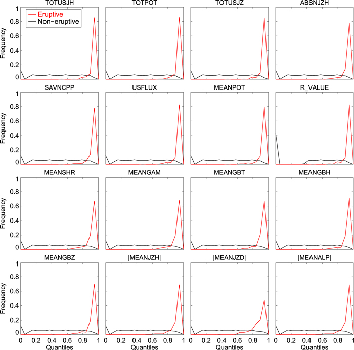
Figure 4. Same as Figure 3 but for modified SHARP parameters.
Download figure:
Standard image High-resolution imageParameters TOTPOT, TOTUSJZ, ABSNJZH, SAVNCPP, USFLUX, MEANPOT, and R_VALUE in both original and modified SHARP data are also effective for discrimination. The rest of the parameters (the third and fourth rows) that perform poorly in discriminating the noneruptive and eruptive ARs have been improved substantially after modification. Thus this modification increases the number of effective SHARP parameters by a factor of two that are able to discriminate the two groups of ARs.
To further evaluate the effectiveness of the modified SHARP parameters for discrimination, we calculate the Fisher ranking score (F-score) for each parameter. The F-score is a useful statistics algorithm that measures both the distance between the data points in different groups and the distance between the data points in the same group for a selected feature (Lomax & Hahs-Vaughn 2013, p.10). For a good predictor, the former should be as large as possible, the latter should be as small as possible. For a binary classification (yes or no outcomes), F-score is defined as,
where x+ and x− are the subsamples of the feature belonging to two groups, respectively. E(x) and Var(x) are the expect value and variance of the samples. A low F-score indicates that the distance between two groups is blunt and there are many nearby values of parameter X related to both groups. Conversely, a high F-score indicates that the distance between two groups is sharp and clear. Similar to Bobra & Couvidat (2015), we calculate the F-score using the SelectKBest class of binary classifier in the Scikit-learn package (Pedregosa et al. 2011).
Figure 5 displays the F-scores for the modified (red dots) and original (black) SHARP parameters. All the modified SHARP parameters have a high F-score, while the F-score is fairly low for more than half of the original SHARP parameters. This once again demonstrates that the modified parameters have been improved significantly in discriminating the two groups of noneruptive and eruptive ARs, which shows potential for them to be used for predicting solar flares.
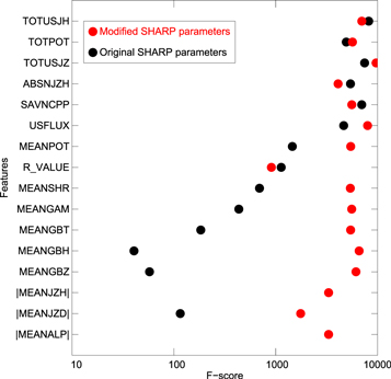
Figure 5. Fisher ranking score (F-score) for each parameter. Black dots refer to the F-scores for the original SHARP parameters; red for the modified SHARP parameters. Names of the parameters are on the Y-axis.
Download figure:
Standard image High-resolution imageIn the aforementioned tests, the original SHARP parameters that perform poorly in discrimination are physical quantities that average over the entire images, i.e., the mean of the quantities. Modification that weighs the PIL areas to the parameters improves their performance significantly. This strongly suggests that the magnetic field property in PILs is tightly related to flare eruptions. This localized property has been significantly diluted when averaging over all of the ARs for the original SHARP parameters.
3.2. Prediction
To assess the potential of predicting flares with the modified SHARP parameters, we use a binary classification method to classify the ARs based on each parameter. We adopt the random forest algorithm using the RandomForestClassifier in the Scikit-learn package (Breiman 2001; Pedregosa et al. 2011). For each AR, the method classifies whether the AR is in the eruptive group or the noneruptive group. To achieve unbiased results, for each parameter we perform a Monte Carlo analysis 500 times on the training and testing processes. For each time, we first shuffle the data points; then we split them into 60% training data set and 40% testing data set; we generate a random forest model based on the training data set to classify ARs; and we run a test on the independent testing data set; finally, we verify the model performance statistically.
As listed in Table 2, compared with the ground truth, this prediction for the AR can be true positive if the prediction agrees with the true and the AR is an eruptive AR, or true negative if the prediction agrees and the AR is a noneruptive AR. The prediction can also be false negative if the prediction disagrees and the AR is eruptive, or false positive if the prediction disagrees and the AR is noneruptive.
Table 2. Confusion Matrix of Binary Classification
| Actual Group | |||
|---|---|---|---|
| Eruptive AR | Noneruptive AR | ||
| Forecast Group | eruptive AR | True positive (TP) | False positive (FP) |
| noneruptive AR | False negative (FN) | True negative (TN) | |
Download table as: ASCIITypeset image
Following Zhang & Casey (2000) and Powers (2011), we use five metrics, recall, precision, F1 Score, True Skill Statistic (TSS), and Heidke Skill Scores (HSS), to evaluate the performance of the prediction. They are defined as,


This binary classifier is deemed to be effective if the metrics are high.
Figure 6 shows metrics for both original (left panel) and modified SHARP parameters (right panel). The black, blue, red, orange, and purple circles represent recall, precision, TSS, HSS, and F1 scores for each parameter, respectively. The horizontal bars in each circle refer to the error bar (standard deviation) for the metrics. The TSS, HSS, and F1 becomes much smaller for half of the original SHARP parameters. Apparently these parameters are not effective classifiers for eruptive and noneruptive ARs. Again these parameters are means of the physical quantities, agreeing with the result in Section 3.1. Performance of these parameters becomes much better for the modified data. This suggests the modified SHARP parameters have great potential to identify the eruptive ARs.

Figure 6. Recall, precision, TSS, HSS, and F1 score (X-axis) for a random forest binary classification for each parameter. Left (right) panel is for the original (modified) parameters. Black, blue, red, orange, and purple circles represent recall, precision, TSS, HSS, and F1, respectively. Short horizontal lines refer to standard deviation for the matrix.
Download figure:
Standard image High-resolution image
Here, the application of the random forest algorithm with a single predictor variable in the above context does not involve many predictors at a time but only one predictor. This does not use the full power of the random forest algorithm. So, results of this numerical application of random forests are not exhaustive and a multiparameter random forest analysis will be done in a future work.
4. Discussion and Conclusions
In this paper, we modify the SDO/HMI SHARP parameters and investigate their potential in discriminating noneruptive and eruptive ARs. The modified SHARP parameters are calculated from the parameter distribution maps after being multiplied with a high-gradient PIL mask. In comparison with the original SHARP parameters, the newly modified ones are more weighed by the PIL mask, and therefore represent the physical quantities in the PIL areas.
We demonstrate that the newly modified SHARP parameters have been improved significantly in discriminating the noneruptive and eruptive ARs. The number of the modified parameters that can well discriminate the eruptive and noneruptive ARs is doubled when compared with the original ones. This suggests that new data have potential to improve the machine-learning-based flare prediction models.
For the newly modified, PIL weighted SHARP parameters, the increase of their ability for discriminating noneruptive and eruptive ARs implies that the high-gradient PIL is tightly linked to solar flares. This provides another piece of evidence in supporting the hypothesis that PIL is an important property of magnetic field to study for advancing our knowledge on the solar eruption mechanisms.
We thank the SDO/HMI team members who have made great contributions to the SDO mission for their hard work! We wish to thank the anonymous referee for valuable suggestions and comments that improved this work significantly. J.W., S.L., and X.A. were supported by the National Natural Science Foundation of China (grant 41604149), Beijing Municipal Science and Technology Project (project Z181100002918004).