


Abstract
By assuming that the solar wind flow is spherically symmetric and that the flow speed becomes constant beyond some critical distance r = R0 (neglecting solar gravitation and acceleration by high coronal temperature), the large-scale solar wind magnetic field lines are distorted into a Parker spiral configuration, which is usually simplified to an Archimedes spiral. Using magnetic field observations near Mercury, Venus, and Earth during solar maximum of Solar Cycle 24, we statistically surveyed the Parker spiral angles and obtained the empirical equations of the Archimedes and Parker spirals by fitting the multiple-point results. We found that the solar wind magnetic field configurations are slightly different during different years. Archimedes and Parker spiral configurations are quite different from each other within 1 au. Our results provide empirical Archimedes and Parker spiral equations that depend on the solar wind velocity and the critical distance (R0). It is inferred that R0 is much larger than that previously assumed. In the near future, the statistical survey of the near-Sun solar wind velocity by Parker Solar Probe can help verify this result.
Export citation and abstract BibTeX RIS
1. Introduction
Since the interplanetary magnetic field (IMF) is frozen in the outflowing solar wind plasma, as a result of the Sun's rotation, the solar wind magnetic field lines are distorted into a so-called Parker spiral configuration (Parker 1958). The solar wind magnetic field exists throughout the entire heliosphere. It is significant for understanding and forecasting space weather to study the structures and dynamics of the solar wind magnetic field. In addition to the Parker model (Parker 1958), many studies have paid attention to the large-scale magnetic field configuration of the solar wind at different heliolatitudes (Owens & Forsyth 2013, and references therein). Note that the solar wind models including nonradial intrinsic magnetic fields and velocities at the source surface were proposed (e.g., Schulte in den Bäumen et al. 2011, 2012). And, recently, Tasnim & Cairns (2016) and Tasnim et al. (2018) suggested more generalized theoretical models including the solar wind's acceleration, conservation of angular momentum, deviations from corotation, and nonradial velocity and magnetic field components from an inner boundary. However, this study focuses on the much more simple and original Parker model, which is capable of describing the large-scale magnetic field of solar wind using long-term averages as mentioned below.
Some assumptions are made to obtain the Parker spiral equation. The solar wind flow is assumed to become radial at the solar source surface, which is a boundary in the Potential-Field Source-Surface model (Altschuler & Newkirk 1969; Schatten et al. 1969) and beyond which, the solar wind magnetic field is assumed to be radial. The source surface is typically placed at 2–2.5 solar radii based on Owens & Forsyth (2013). After coming out from the source surface, the solar wind flow is assumed to be spherically symmetric. And there exists a critical distance (R0), beyond which both solar gravitation and acceleration by high coronal temperature can be neglected and the solar wind velocity becomes constant (Parker 1958). The constant solar wind velocity is represented as vm in the following equations. As the plasma streamline and the frozen-in field line coincide, Parker (1958) concluded that the solar wind magnetic field at the point (r, θ, ϕ) in spherical coordinates are
where ω is the Sun's angular velocity, which is approximately 2.7 × 10⁻⁶ rad s−1. ϕ0 is the azimuth angle and B(θ, ϕ0) is the magnetic field at r = R0. The radial component Br of the field is proportional to  and the tangential component Bϕ of the field is proportional to 1/r at large distance r (r ≫ R0). The solar wind magnetic field generates a spiral geometry due to both the radial and tangential components. The equation of the solar wind magnetic field line can be written as:
This equation as derived by Parker (1958) shows that the Parker spiral angle ϕ increases with increasing r when ω, vm, R0, and ϕ0 are constants. However, ϕ0 corresponds to the distance r = R0, and we do not know exactly what ϕ0 and R0 are yet. By changing the form of Equation (2), we can obtain
or

where  .
.
In general, the Parker spiral IMF line at large r ( is negligible with respect to
  ) can be simplified as an Archimedes spiral, whose general form is given by

By comparing Equations (4) and (5), it can be seen that  and
and  . However, Equation (4) is quite different from Equation (5) for small r, which means that Archimedes spiral configuration and Parker spiral configuration are not the same when the distance from the Sun is not large enough.
The Parker spiral angle is defined by the angle between the x component (pointing to the Sun) and the y component (pointing to the opposite direction of the planetary motion) of the IMF (Luhmann et al. 1993; Masunaga et al. 2013), negative for −By components and positive for +By components. Parker's theory has been roughly verified by using data from Helios, MESSENGER, Ulysses, Mariner 4, Mariner 5, Pioneer 6, Pioneer 10, and Mariner 10, which primary science orbits range from 0.29 to 5 au (Behannon 1978; Forsyth et al. 1996; Korth et al. 2011). Thomas & Smith (1980) surveyed the Parker spiral configuration of the solar wind magnetic field between 1 and 8.5 au measured by Pioneer 10 and 11 and found that the average direction is basically in accordance with Parker's predictions. It is difficult to investigate the Parker spiral tendency instantaneously because of the large fluctuations of the solar wind magnetic field (Borovsky 2010). Using Ulysses magnetic field observations, Forsyth et al. (1996) found the magnetic field can be hardly described by the Parker model for instantaneously averaged measurements, instead varying greatly in direction and magnitude. The solar wind magnetic field is approximately consistent with Parker's theory but there are large fluctuations in the field. Consequently, long-term statistical studies of the IMF on average are able to help investigate the large-scale configuration of the solar wind magnetic field.
Previous studies have confirmed that the Parker spiral angle varies with the heliocentric distance. Korth et al. (2011) found that the main concentration of the spiral angle distributions near Mercury is about 30° by Helios and MESSENGER observations. Svalgaard & Wilcox (1974) showed that the spiral angle near Earth was approximately 45°, which was predicted by Parker's theory. They also pointed out that there is a variation in the spiral angle with sunspot cycle. Luhmann et al. (1993) reported that the Parker spiral angles at 0.72 and 1 au decrease slightly from the declining phase through solar minimum during Cycle 21. Borovsky (2010) also found that there is no clear solar cycle dependence of the IMF direction at 1 au by analyzing OMNI2 and Advanced Composition Explorer (ACE) measurements over four solar cycles. A recent study shows that the IMF direction near Venus is affected by solar cycles but not significantly affected by solar phases of the same solar cycle (Chang et al. 2018).
Although the Parker spiral configuration of the solar wind magnetic field has been accepted widely, the exact equations of the Parker or Archimedes spirals have not been obtained yet. In this study, we model the empirical configuration of solar wind magnetic field to derive the specific Parker and Archimedes spirals using multiple-point observations during solar maximum of Cycle 24 within 1 au. Furthermore, we can infer the critical distance, R0, and the constant average speed, vm, which can help us understand the acceleration of the solar wind.
2. Data and Instrumentation
The data used in this study are provided by magnetometers (MAG) on board MESSENGER (Anderson et al. 2007; Solomon et al. 2007), Venus Express (VEX; Svedhem et al. 2007; Zhang et al. 2007), ACE (Smith et al. 1998; Stone et al. 1998), and Wind (Lepping et al. 1995; Ogilvie & Desch 1997), since these four spacecraft covered the same time duration of the maximum phase of Solar Cycle 24. MESSENGER was launched on 2004 August 3, inserted into the Mercury orbit on 2011 March 18, and deorbited on 2015 April 30. VEX was launched on 2005 November 9, arrived at Venus on 2006 April 11, and deorbited on 2015 January 18. However, it lost contact on 2014 November 28, leading to the data gap afterwards. The ACE spacecraft was launched on 1997 August 25 and has been orbiting around the Lagrange point 1 (L1) (∼240 RE sunward of Earth) of the Sun–Earth system (Stone et al. 1998). The Wind spacecraft was launched on 1994 November 1 and positioned at L1 since 2004 (Wood et al. 2015; Ogilvie & Desch 1997). The MAG data observed by MESSENGER and Wind from 2012 January to 2014 November and by VEX and ACE from 2008 January to 2014 November are used.
However, the resolutions of these four MAG measurements used in this study are quite different: the 60 s resolution by MESSENGER, the 1 s resolution by VEX, the 16 s resolution by ACE, and the 3 s resolution by Wind. Note that the MESSENGER and VEX spacecraft entered into the magnetosphere of Mercury and the induced magnetosphere of Venus, respectively, during every orbit. The magnetic field configurations of the magnetosphere are totally different from that of the solar wind. Therefore, the magnetic field measurements in the two planets' magnetosphere have been removed. For each orbit, we removed all the measurements during the interval from half an hour prior to the inbound bow shock to half an hour after the outbound bow shock. Since the resolutions of the solar wind magnetic field data obtained by these four spacecraft are quite different, we chose a relatively long time interval, 30 minutes, for averaging all the three spacecraft MAG data. The solar wind usually consists of Alfvénic turbulence, which covers a broad band of wavelength. Therefore, a relatively long interval is needed to cover as many as Alfvén waves as possible.However, this time interval cannot be very long, say several hours, otherwise there would be very few samples for each orbit of MESSENGER with a period of about 12 hr. On the other hand, large-scale solar wind structures with very different magnetic field configurations from the Parker spiral can last from several hours to several days within 1 au. The samples of magnetic field smoothed during these structures can greatly deviate from Parker spiral configuration. Therefore, long-term measurements are required to reduce such deviations by average.
It should be emphasized that the solar wind magnetic field data must cover the same time duration so that we can reduce as much as possible the influence of the solar activity. In this study, relatively long-term solar wind MAG data measured by MESSENGER, VEX, ACE, and Wind cover the same time duration from 2012 January to 2014 November, which covers most of the maximum phase of Solar Cycle 24. Unfortunately, there are no relatively long-term solar wind magnetic field measurements during that period from other planets beyond 1 au.
3. Observation
Now we show the statistical results of the solar wind magnetic field from the measurements by MESSENGER, VEX, ACE, and Wind. The Parker spiral angles near Mercury, Venus, and Earth are investigated to obtain the empirical equations of the Archimedes and Parker spiral configurations at the solar maximum of Cycle 24. Furthermore, R0 and the corresponding solar wind average velocity vm are also inferred.
3.1. MESSENGER Observations near Mercury
The perihelion and the aphelion of Mercury are about 0.31 au and 0.47 au, respectively. Since the heliocentric distance of MESSENGER varies too much in percentage (over 50%), we divide the solar wind magnetic field data near Mercury into two parts by the distance from the Sun (too many parts would cause the measurements to not be long enough). The Mercury-centered solar orbital (MSO) coordinate system is used in MESSENGER observations: +X points from Mercury to the Sun; +Y is defined to be antiparallel to the direction of Mercury orbital motion; +Z is normal to the X–Y plane, completing a right-handed system. Figures 1(a)–(d) show the distributions of the occurrence of the Parker spiral angle from 0.31 to 0.39 au measured by MESSENGER during 2012, 2013, 2014, and solar maximum, respectively. We model the distribution by Gaussian function:

In this equation, a is the peak of the fitting curve, b is the corresponding position of the peak and c is the standard deviation. The two curves (red and magenta curves) in each figure represent two respective Gaussian fittings for two opposite directions of the IMF: one is the direction toward the Sun, and the other is away from the Sun. There are two peaks at different positions (including a negative value b1 and a positive value b2), which correspond to two average Parker angles toward and away from the Sun. The included angle is the angle between these two average opposite directions of the IMF. If the Parker spiral is stable and most fluctuations of IMF are removed, the included angle is expected to be 180°. In Figure 1, the negative values of b1 are −22 52, −2452, −2178, and −2288. The positive values of b2 are 15920, 16050, 15810, and 15910. Thus, the included angles between the two IMF directions are 18172, 18502, 17988, and 18198. They are very close to 180°, which is similar to that obtained near Mercury (Korth et al. 2011). Since we only focus on the configuration rather than the direction of the magnetic field, the average Parker spiral angle (ϕ) is defined by
  and are calculated to be 2166, 2201, 2184, and 2189 in Figures 1(a)–(d).
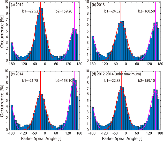
Figure 1. Histograms of the occurrence of the Parker angle between 0.31 au and 0.39 au observed by MESSENGER. (a)–(c) Observations during 2012–2014, respectively. (d) Observations during solar maximum (2012–2014).
Download figure:
Standard image High-resolution imageSimilarly, Figure 2 displays distributions of the occurrence of the Parker angle during solar maximum using data between 0.39 and 0.47 au. Figure 2 also presents the b1 and b2 derived by Gaussian fitting. As a result, the corresponding average Parker angles between 0.39 and 0.47 au during 2012, 2013, 2014, and solar maximum can be calculated to be 2657, 2734, 2536, and 2682, respectively. It is clear that the average Parker angles between 0.39 and 0.47 au are much greater than those between 0.31 and 0.39 au. This result is in accordance with Equation (2), which shows that ϕ increases with increasing r.

Figure 2. Histograms of the occurrence of the Parker angle between 0.39 au and 0.47 au observed by MESSENGER. (a)–(c) Observations during 2012–2014, respectively. (d) Observations during solar maximum (2012–2014).
Download figure:
Standard image High-resolution image3.2. VEX Observations near Venus
The Venus solar orbital (VSO) coordinate system, similar to the MSO coordinate system at Mercury, is used for studying the solar wind magnetic field near Venus measured by VEX. The VSO system has its X-axis pointing from Venus toward the Sun and its Y-axis pointing in the opposite direction of Venus orbital motion. The Z-axis is perpendicular to Venus's orbital plane, forming a right-handed system. Figure 3 shows the distributions of the occurrence of the Parker angle at 0.72 au during different years (2008–2014) by VEX observations. The 7 yr observations as shown in Figures 3(a)–(g) are plotted year by year. The negative b1 varies from −4648 to −3636 during these 7 yr and the average value is −4125 for the IMF toward the Sun. The positive b2 varies from 12810 to 14460 during these 7 yr and the average value is 13747 for the IMF away from the Sun. The included angle of these two IMF directions is about 17872, which is very close to 180°. Figures 3(h) and (i) show the occurrence of Parker angle during solar minimum and solar maximum, respectively. To clearly display the variation of the Parker angle, Figure 4 concludes all relevant angles that are plotted according to Figure 3. The average Parker angles (the average Parker angles during 2008–2014 are marked by red cycles, and the average Parker angles during solar minimum and maximum are marked by red asterisks) and the corresponding b1 and b2 (yearly b1 and b2 are marked by blue cycles, and b1 and b2 during solar minimum and maximum are marked by blue asterisks) are displayed in Figure 4(a). It can be seen that there are significant differences in b1 and b2 from year to year, suggesting that the average Parker angle also has a yearly variation. The average Parker angles are 4207 at solar minimum and 4200 at solar maximum, indicating that the average Parker angle is not significantly affected by solar activity. Figure 4(b) shows the included angles (b2–b1 in Figure 3) of the IMF toward the Sun and away from the Sun. The included angles are 18393 during solar minimum and 17599 during solar maximum, which are very close to 180°. Most of the included angles from 2008 to 2014 are around 180° ranging from 17622 to 18672. However, it is worth noting that the include angle during 2012 is 16446, much smaller than 180°. Because the reason for this is not clear to us, we insist on using long-term measurements to reduce as much as possible the potential influences by turbulence, solar eruptions, and so on.
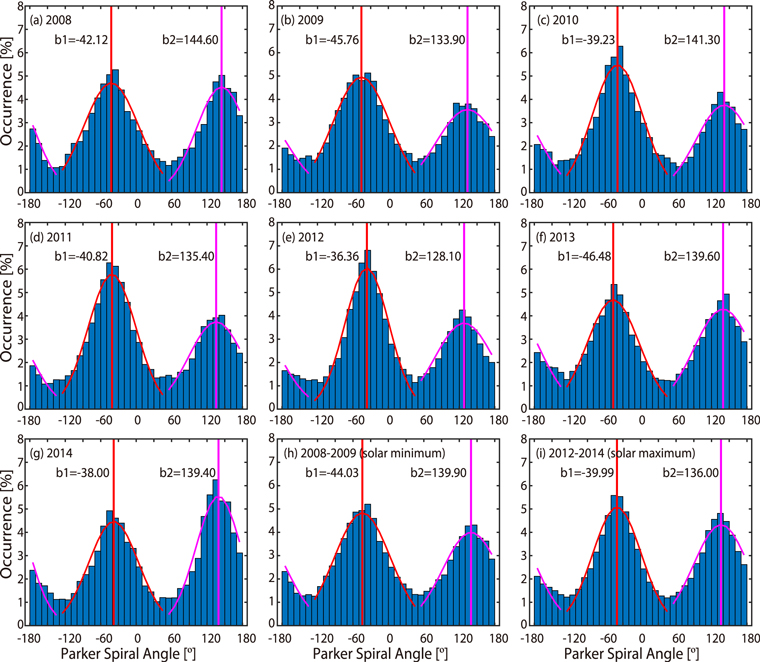
Figure 3. Histograms of the occurrence of the Parker angle at 0.72 au during different years (2008–2014) using data obtained by VEX. (a)–(g) Observations during 2008–2014, respectively. (h)–(i) Observations during solar minimum (2008–2009) and solar maximum (2012–2014), respectively.
Download figure:
Standard image High-resolution image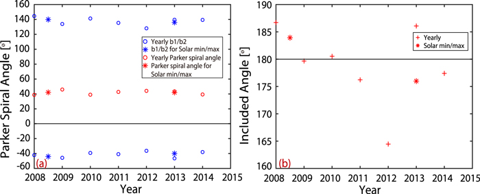
Figure 4. Distributions of b1, b2, the average Parker angles, and the included angles observed by VEX. (a) b1/b2 during 2008–2014 (blue circles), b1/b2 during solar minimum and maximum (blue asterisks), the average Parker angles during 2008–2014 (red circles) and the average Parker angles during solar minimum and maximum (red asterisks) are displayed. (b) The included angle between the average inward and outward IMF directions.
Download figure:
Standard image High-resolution image3.3. ACE and Wind Observations near Earth
The ACE and Wind MAG measurements are investigated in a Geocentric solar ecliptic coordinate system that is similar to MSO and VSO systems. Analogous to Figure 3, Figure 5 shows the distributions of the Parker angle at 1 au during different years (2008–2014) by ACE observations. The negative b1 varies from −4881 to −4014 during 2008 to 2014 and the average value is −4466. The positive b2 varies from 12530 to 13790 during these 7 yr and the average value of b2 is 13037. Figures 5(h) and (i) show occurrences of Parker angle during solar minimum and maximum, respectively. Figure 6 concludes all relevant angles similar to Figure 4. The average Parker angles and the corresponding b1 and b2 in Figure 5 are displayed in Figure 6(a). The average Parker angle is 4530 during solar minimum and 4911 during solar maximum. However, the average Parker angles from 2008 to 2014 perform no significant dependence on solar activity. Figure 6(b) shows the included angles of the inward and outward IMF. The included angles are 17580 during solar minimum and 17502 during solar maximum. It should be pointed out that our results are better than those obtained in previous studies (Svalgaard & Wilcox 1974; Thomas & Smith 1980). One of the reasons could be that we used much more data in this study. As mentioned above, Wind is also positioned at L1 during solar maximum of Solar Cycle 24. Figure 7 shows the distributions of the Parker angle at 1 au during different years (2012–2014) using data obtained by Wind. Table 1 lists the average Parker angles and the average included angles measured by ACE and Wind during solar maximum in detail. Compared to the average Parker angles measured by ACE, the angles measured by Wind during 2012, 2013, 2014, and solar maximum increase by 1.91%, 2.73%, 4.85%, and 3.22%, respectively. The included angles observed by both ACE and Wind are very close to 180°, which also implies that the data we used are reliable. Since ACE and Wind are both positioned at L1, the average Parker angles measured by Wind are in good agreement with those measured by ACE. Due to the tiny differences of the observations between the ACE and WIND, we use ACE data at 1 au to model the solar wind magnetic field configuration in the next section.
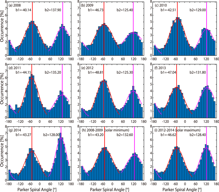
Figure 5. Histograms of the occurrence of the Parker angle at 1 au during different years (2008–2014) using data obtained by ACE. (a)–(g) Observations during 2008–2014, respectively. (h)–(i) Observations during solar minimum (2008–2009) and solar maximum (2012–2014), respectively.
Download figure:
Standard image High-resolution image
Figure 6. Distributions of b1, b2, the average Parker angles, and the included angles observed by ACE. (a) b1/b2 during 2008–2014 (blue circles), b1/b2 during solar minimum and maximum (blue asterisks), the average Parker angles during 2008–2014 (red circles), and the average Parker angles during solar minimum and maximum (red asterisks) are displayed. (b) The included angle between the average inward and outward IMF directions.
Download figure:
Standard image High-resolution image
Figure 7. Histograms of the occurrence of the Parker angle at 1 au during different years (2012–2014) using data obtained by Wind. (a)–(c) Observations during 2012 to 2014, respectively. (d) Observations during solar maximum (2012–2014).
Download figure:
Standard image High-resolution imageTable 1. The Average Parker Angles and the Average Included Angles Observed by ACE and Wind during Solar Maximum (2012–2014)
| Period | 2012 | 2013 | 2014 | Solar Maximum | |
|---|---|---|---|---|---|
| The average Parker angle | ACE | 5176 |
4762 |
4764 |
4911 |
| WIND | 5275 |
4892 |
4995 |
5069 |
|
| The average included angle | ACE | 17411 |
17884 |
17127 |
17502 |
| WIND | 17830 |
18423 |
17589 |
17978 |
|
Download table as: ASCIITypeset image
4. Multiple-point Modeling the Parker Spiral Configuration
As mentioned above, Parker and Archimedes spiral configurations are quite different from each other when the heliocentric distance is not large enough. The Parker spiral can be simplified to be Archimedes spiral only when  is negligible with respect to
  in Equation (4). Here, we believe
  can be neglected when
  . The quantitative difference between Equations (4) and (5) (Δϕ or Δϕ/ϕ) depends on not only R0 but also vm, and thus is too complicated to display when the Parker and Archimedes spirals are equivalent. On the contrary, with a given R0,
  can easily indicate beyond which r (under a specific R0), the Parker spiral can be simplified to Archimedes spiral though we do not know the exact forms of these two spirals. Therefore, the
  , which is a function of R0, is a good parameter to indicate whether the Parker spiral can be simplified as the Archimedes spiral. Figure 8 shows the parameter
  with different R0s varying with the distance to the Sun. Since there is a strong dependence on R0, four different R0 (7.19 Rs, 15 Rs, 30 Rs, and 45 Rs) marked by different colors are plotted. For each curve,
  increases at first to reach a peak at
  and then descends with increasing r. It can be easily seen that all the curves with different R0 have the same profiles. It is obvious that
  is significantly greater than 10% (marked by the red line in Figure 8) for
  within 1 au, suggesting that
  cannot be ignored with respect to r' within 1 au. In other words, the Parker spiral cannot be simplified to the Archimedes spiral within 1 au. Here we will model both the Parker and Archimedes spirals by Equations (4) and (5) using the average Parker angles at 0.35 au (0.31–0.39 au, observed by MESSENGER), 0.43 au (0.39–0.47 au, observed by MESSENGER), 0.72 au (observed by VEX), and 1 au (observed by ACE).

Figure 8. Variation of  with the distance to the Sun (r). The horizontal axis is r (in logarithmic coordinate) and the vertical axis is
  (1 au is about
  and the average distance between Mercury and the Sun is 0.39 au).
Download figure:
Standard image High-resolution imageFigures 9(a)–(d) show the solar wind magnetic field configurations by Parker and Archimedes spiral modelings during 2012, 2013, 2014, and solar maximum, respectively. Based on these four points, we can simply model Archimedes spiral configuration (Equation (5)) using the fitting method of the minimal standard error (σ is given by  , where ϕi is the Parker angle calculated from the Parker or Archimedes equation and
  is the Parker angle from observations). The final results are marked by red curves in Figures 9(a)–(e). The fitting of the Archimedes spiral provides us with the two coefficients (a0 and b0) of Equation (5), with which we can derive vm from
  . Since the Parker spiral cannot be simplified to the Archimedes spiral within 1 au, the Archimedes spiral obtained here is just an empirical model that cannot reveal the physical features of the solar wind magnetic field configuration. For instance, the a0 is about 0.7617 during solar maximum, and then vm is 530.28 km s−1, which is too large for the real average solar wind velocity (415.07 km s−1) measured by ACE during solar maximum.
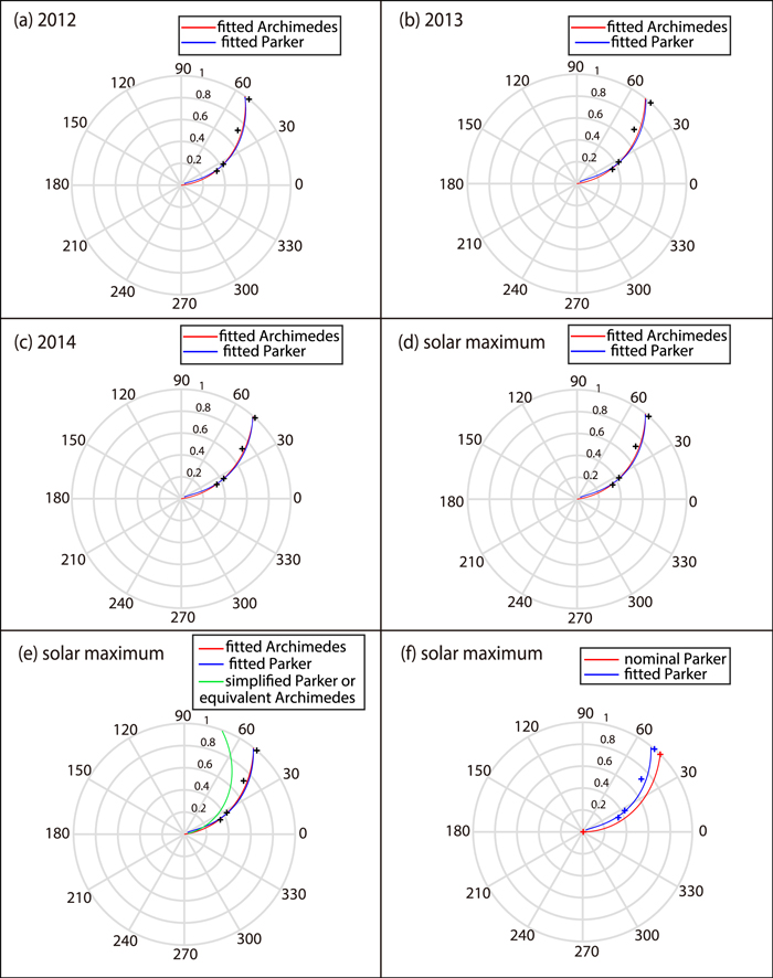
Figure 9. Solar wind magnetic field configurations and their comparisons within 1 au. (a)–(d) The solar wind magnetic field configurations fitted by Parker and Archimedes spirals during 2012, 2013, 2014, and solar maximum, respectively. (e) The solar wind magnetic field configurations fitted by Parker and Archimedes spirals, and the simplified Parker spiral during solar maximum. (f) The comparison between the nominal and our fitted Parker spiral during solar maximum.
Download figure:
Standard image High-resolution imageThe fitting of the Parker spiral is much more complicated since Equation (4) cannot be transformed into a linear equation. We first need to assume a proper ϕ0. Here we assume that the solar wind starts to be accelerated from the source surface at r = 2.5 Rs based on Hoeksema & Scherrer (1986) and reaches a constant average speed at r = R0. We further assume that the solar wind undergoes an acceleration process with constant acceleration, i.e., the average speed ( ) from r = 2.5 Rs to r = R0 is
  . ϕ0 is thus given by
Then, the standard error (σ) depending on R0 and vm can be derived. The minimal standard error (σmin) for each time interval can provide the unique pair of R0 and vm. And thus the Parker spiral can be determined by the assumed ϕ0 and derived R0 and vm from the fitting. The blue curves in Figure 9 mark the final Parker spiral configurations during different time intervals. In Figure 9(e), a green line representing the simplified Parker spiral (to an equivalent Archimedes spiral) is added during solar maximum for comparison. It is obvious that the Parker spiral cannot be simplified to the Archimedes spiral as revealed by Figure 8. We also compared the nominal Parker spiral and our fitted Parker spiral in Figure 9(f). The nominal Parker spiral is actually an Archimedes spiral with an angle of 45° at 1 au and ϕ0 = 0 at r = Rs (e.g., Schulte in den Bäumen et al. 2011). From Figure 9(f), we can see that our fitted Parker spiral has a larger azimuthal component of magnetic field at 1 au.
In summary, Table 2 concludes the fitting results of the Parker and Archimedes spirals for the assumed ϕ0 by Equation (7). It is important to note that the fitting results of R0 for the Parker spiral during different intervals are all larger than 30 Rs, which is much greater than that assumed by Parker (1958). And the corresponding solar wind velocities are close to the observations by ACE.
Table 2. Fitting Results
| Period | 2012 | 2013 | 2014 | Solar Maximum | |
|---|---|---|---|---|---|
Archimedes spiral equation ( ) ) |

|
0.0386 | 0.0504 | 0.0201 | 0.0333 |
| a0 | 0.8528 | 0.7539 | 0.7144 | 0.7617 | |
| b0 | 0.0959 | 0.1415 | 0.1388 | 0.1340 | |
Parker spiral equation 
|

|
0.0471 | 0.0592 | 0.0292 | 0.0428 |

|
34 | 42 | 40 | 39 | |

|
358.32 | 387.95 | 399.55 | 381.21 | |
Download table as: ASCIITypeset image
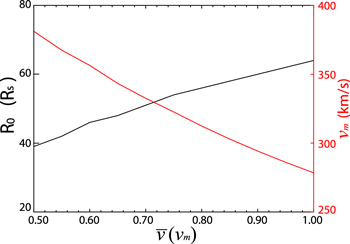
Note that different ϕ0 can change the fitting results of vm and R0. Figure 10 shows the variations of vm and R0 depending on the hypothetical average speed ( ) from the source surface the critical distance R0.
  is assumed to stay between
  and vm (Parker 1965) because the solar wind actually undergoes an acceleration process with decreasing accelerations near the Sun. ϕ0 is thus between
  and
and  . It is obvious from Figure 10 that R0 increases and vm decreases with increasing
  . Therefore, the fitted 39 Rs during solar maximum as shown in Table 2 is a lower limit of R0.
Figure 10. Dependence of R0 and vm on  during solar maximum.
Download figure:
Standard image High-resolution image
5. Discussion and Conclusions
We statistically studied the solar wind magnetic field directions measured by MESSENGER, VEX, ACE, and Wind and obtained the Parker angles within 1 au during the solar maximum of Solar Cycle 24. Because ω, vm, R0, and ϕ0 can be seen as constants in a long-term period, the distance from the Sun r becomes the most dominant factor for the IMF direction. Unlike Thomas & Smith (1980) who used the median and Svalgaard & Wilcox (1974) who used the average when discussing the Parker angle, we model the distribution of the occurrence by Gaussian function to calculate the Parker angle. In this way, we obtained the Parker angles at four different positions (0.35, 0.43, 0.72, and 1 au). The average Parker angle is increasing from Mercury to Earth as predicted by Parker (1958) and appears to have a slight dependence on solar activity. The Parker angles of these four points enable us to fit the average solar wind magnetic field configuration within 1 au during the maximum phase of Solar Cycle 24. To the best of our knowledge, most previous studies are performed using single-satellite observations. They focused on the values of the Parker spiral angles at different heliocentric distances and their dependencies on the solar cycle. The nominal Parker spiral, whose Parker angle is 45° at 1 au, is usually thought to be linearly dependent on heliocentric distance or an Archimedes spiral (e.g., Schulte in den Bäumen et al. 2012). Our study for the first time clearly pointed out that the Parker spiral cannot usually be simplified to the Archimedes spiral especially within 1 au. And by using multiple-point observations, we obtained the exact equation of Parker spiral with known empirical coefficients. In addition, our multiple-point Parker model can infer the value of the critical distance, R0.
Our results of the solar wind magnetic field configuration during maximum phase of Solar Cycle 24 can be concluded as follows. The modeled Parker spiral is  (
( and ϕ is in unit of rad) and the Archimedes spiral is
  (r is in astronomical units and ϕ is in units of rad). It is clear that the parameters of these two spiral configurations are significantly different from each other during the same period. In fact, the Archimedes spiral has no definite physical meaning. It is a coincidence that the minimal standard errors in Archimedes spiral modeling are much lower than that in Parker spiral modeling. Based on the fitting results of the Parker spiral configuration, R0 is inferred to be over 39 Rs, which is much larger than that (7.19 Rs) assumed by Parker (1958). A much larger R0 indicates that the solar wind acceleration could be a significantly longer process. In the near future, the Parker Solar Probe can provide us with long-term observations near the Sun (Fox et al. 2016) to verify this result.
As we pointed out above, no suitable solar wind magnetic filed data during the same period from spacecraft near planets beyond 1 au are used in this study. Therefore, our empirical models of the Parker and Archimedes spirals are probably not applicable for solar wind magnetic field beyond 1 au.
We acknowledge MESSENGER and Venus Express teams as well as the NASA Planetary Data System (http://ppi.pds.nasa.gov) for providing the data. We also thank ACE and Wind teams and NASA CDAWeb for providing magnetometer data at 1 au. This work is funded by The Science and Technology Development Fund, Macao SAR (File no. 008/2016/A1) and National Natural Science Foundation of China (NSFC) under grants 41564007 and 41731067.