


Abstract
Spectrometers provide our most detailed diagnostics of the solar coronal plasma, and spectral data is routinely used to measure the temperature, density, and flow velocity in coronal features. However, spectrographs suffer from a limited instantaneous field of view (IFOV). Conversely, imaging instruments can provide a relatively large IFOV, but extreme-ultraviolet (EUV) multilayer imaging offers very limited spectral resolution. In this paper, we suggest an instrument concept that combines the large IFOV of an imager with the diagnostic capability of a spectrograph, develop a new parametric model to describe the instrument, and evaluate a new method for "deconvolving" the data from such an instrument. To demonstrate the operating principle of this new slitless spectroscopy instrument, actual spectroscopic raster data from the Hinode/EUV Imaging Spectrometer (EIS) spectrometer is used. We assume that observations in multiple spectral orders are obtained, and then use a new inverse problem method to infer the spectral properties. Unlike previous methods, physical constraints and regularization derived from prior knowledge can be naturally incorporated as part of the solution process. We find that the fidelity of the solution is vastly improved compared to previous methods. The errors are typically only a few km s−1 over a large IFOV, with a width of a few hundred pixels and an arbitrarily large height. These errors are not much larger than the errors in current slit spectroscopic instruments with limited IFOV. A further benefit is that the performance of candidate instruments can be optimized for specific scientific objectives. We demonstrate this by deriving optimum values for the spectral dispersion and signal-to-noise ratio.
Export citation and abstract BibTeX RIS
1. Introduction
Spectrographs provide a unique window into plasma parameters in the solar atmosphere (Phillips et al. 2008). In the corona, and elsewhere, spectral emission line profiles have been used to infer microturbulence velocities (Coyner & Davila 2011), Doppler shifts have been used to measure flows (Brosius et al. 2000a), and line intensity ratios have been used to measure temperatures and densities (Brosius et al. 2000b). In fact, by fitting the emission line profile to obtain the line intensity, Doppler shift, and width, spectrographs provide the most accurate measurements of solar plasma characteristics such as density, temperature, and flow speed, and provide essential information for understanding dynamic solar phenomena. However, traditionally the usefulness of spectrographic instruments has been limited by a small instantaneous field of view (IFOV), i.e., the inability to cover large spatial regions of the Sun quickly using a narrow slit.
Imaging instruments, on the other hand, are able to provide high time and spatial resolution images of large regions of the solar disk but with limited spectral resolution. Multilayer extreme-ultraviolet (EUV) telescopes like those on board the Solar Dynamics Observatory (SDO; Haisch et al. 1988; Lemen et al. 2012) can now obtain a full disk solar image every 10 s with roughly 1'' spatial resolution. However, multilayer imagers typically have a FWHM spectral resolving power λ/δλ of about 50. For example, the spectral resolving power of the Atmospheric Imaging Assembly (AIA) on SDO varies with bandpass but is of order 30–70 in the EUV (Boerner et al. 2012). In contrast, a typical solar EUV spectrograph (Brosius et al. 2000a) has a spectral resolving power of order 5000 in the EUV. Because of the low spectral resolving power, it is difficult to interpret multilayer imaging data to accurately obtain plasma parameters like temperature and density. In addition, there is no unambiguous measure of plasma flow velocity. Proper motions observed in imagers are usually interpreted as flows perpendicular to the line of sight, but proper motions due to actual plasma flow can be confused with the evolution of temperature and density within the source as plasma emissivity increases or decreases in a particular bandpass. This ambiguity can be reduced by taking images of the same scene in different bandpasses; however, one then sacrifices simultaneity.
In the past, typically two strategies have been employed to overcome the limited IFOV of slit spectrographs; (1) the slit is rastered over the area of interest with an exposure taken at each pointing location, or (2) a wider aperture, a slot, is used to image a two-dimensional (2D) region on the Sun. In the first strategy (see Figure 1), the raster process can easily take 10 minutes or longer to cover an active region sized area on the Sun, and this time becomes longer as the spatial resolution is increased (i.e., slit width decreased) or the rastered area is increased. Because of this long raster cycle time, the spectra of dynamic events like flares, coronal mass ejections (CMEs), or transient brightening are obtained only rarely. And even if spectra are obtained, they are either taken over an extremely small spatial region so that the overall context is not apparent, or the spectra are not co-temporal across the raster, adding uncertainty to the analysis.

Figure 1. Slit spectrograph schematic. An imaging unit (e.g., telescope, mirror) focuses a 2D scene on an image plane. A narrow slit lies on the image plane to limit the FOV to a 1D portion of the scene. The light that passes through the slit is input to a wavelength dispersive unit, which generally consists of collimator optics (e.g., mirror), a dispersive element (e.g., diffraction grating), and focusing optics (e.g., mirror). Each spectral line in the incoming light is dispersed according to the wavelength and imaged onto a 2D detector. To obtain the spectrum of the entire 2D scene, the slit is moved within the image plane to scan the scene spatially.
Download figure:
Standard image High-resolution imageAn alternate strategy to rastering is to widen the slit to become what is usually called a slot, but slot images have traditionally been difficult to interpret (Brosius et al. 1993). Coronal emission lines have a finite line width, Δλ (Coyner & Davila 2011). Because of this, the observed intensity in any one spatial position depends on the intensity at that position, plus the spectrally dispersed contributions from neighboring positions. More details on this process are presented in Section 2 below. This dispersion within the slot image creates difficulty in inferring the spectral line profile at each position due to overlapping spectra from adjacent spatial positions, and degrades the spatial resolution of the zero-order image itself. Another difficulty with slot images is that emission lines nearby in wavelength can cause the overlapping of the individual slot images (Figure 2). For example, the S082A spectroheliograph on board Skylab produced full disk emission line images of the Sun in a slitless instrument (Tousey et al. 1977) with a moderately high spectral resolution. These images provided significant insight into a broad range of solar coronal emission, but the overlapping of the images made detailed analysis of the data almost impossible, except for spatially compact sources. Solar EUV Rocket Telescope and Spectrograph (SERTS) and EIS partially addressed this problem by using a slot to produce monochromatic images with a more limited FOV to reduce the occurrence of overlapping spectral lines. Again, however, dispersion within the slot image prevented the detailed analysis for intensity, Doppler shift, and line width at each spatial position in the wide slit, except for spatially compact sources.

Figure 2. When the slit of an imaging spectrograph is widened to a slot, monochromatic dispersed images of the slot are reproduced at the detector for each emission line in the source. Depending on the size of the FOV, the dispersion of the spectrograph, and the wavelengths of the emission lines (e.g., λ1, λ2, and λs) as shown, these monochromatic images may appear as separate images or overlap on the detector.
Download figure:
Standard image High-resolution imageKankelborg & Thomas (2001) introduced the idea of using multiple images, −1, 0, and +1 spectral orders of a single emission line, to provide data to "deconvolve" the slot image into individual spectral line contributions. This scheme provided three independent images to measure the three spectral line parameters (intensity, Doppler shift, and width) at each spatial position. Subsequently the Multi-Order Solar EUV Spectrograph (MOSES) instrument was designed and flown on a sounding rocket to provide the 0, +1, and −1 order images. The images were analyzed using Fourier back projection, pixon reconstruction, and Smooth Multiplicative Algebraic Reconstruction (SMART) algorithms (Fox et al. 2003; Harra et al. 2005; Fox et al. 2010). From simulation results, SMART was regarded as the most successful one, yielding ∼1/4 pixel precision in Doppler shifts and ∼1/3 pixel precision in line widths where one MOSES pixel is ∼29 mÅ (Fox 2011). These initial inversion results demonstrated the usefulness of a multi-order slitless spectrometer for extracting spectral line parameters in a 2D FOV. However there were at least two significant issues; (1) the SMART method introduces significant artifacts into the reconstruction including the systematic under- or over-estimation of parameters and over-smoothing (Fox 2011) because the inverse problem posed in a non-parametric way is heavily underdetermined, and (2) it is difficult to introduce constraints (derived from prior knowledge) to improve the solution. Hence a more powerful inversion method is needed. The method should be flexible enough to allow (1) the use of an arbitrary combination of multiple spectral orders that can be tailored to the scientific objective and the resource allocations of the instrument, and (2) the introduction of reasonable constraints on the inversion without imposing artificial smoothing while minimizing the numerical artifacts in the resultant inversion.
In this paper, a new parametric model is developed that describes the formation of a dispersed EUV image of the solar corona in terms of the emission line parameters in the source, i.e., the integrated intensity and the normalized line profile, for each pixel. Like Kankelborg & Thomas (2001), we consider images obtained over a 2D FOV and at multiple spectral (diffraction) orders within a spectrograph. We then study the problem of estimating emission line parameters from these images of the slitless spectrometer. For this, we consider the "deconvolution" of a series of artificial images generated with parameters similar to those observed by Hinode/EIS. The numerical problem is solved iteratively by choosing emission line parameters that minimize the difference between the observed image and the reconstructed image subject to reasonable constraints, and with proper regularization derived from prior knowledge. Initial results show that the typical Doppler shift and line width are recovered by the reconstruction method with an error of order a few km s−1 at wavelengths similar to those observed with Hinode/EIS. This method allows the natural incorporation of physical bounds, constraints, and regularization conditions.
In Section 2, we first describe the parametric model for the dispersed images of the slitless spectrometer, and then formulate the inverse problem as an optimization problem in Section 3. In Section 4, we use data from the Hinode/EIS instrument to model the line profile parameters as random variables, which is then used to simulate the measurements of the slitless spectrometer as well as to constrain the inverse problem. We then consider numerical solution of the problem using simulated realistic solar parameters derived from Hinode/EIS spectrometer raster observations, and discuss the optimization of regularization parameters and the instrument design. Finally we discuss the results and conclusions in Section 5.
An instrument designed to use this new parametric deconvolution method would have the ability to reliably obtain spectral line parameters at every pixel in a 2D FOV, and thus allowing new spectroscopic observations of solar transient events. These observations would provide a new insight into flares, CMEs, and other rapidly evolving solar structures, and hence facilitate the understanding of transient solar phenomena. Therefore, this paper will lay the foundation for a new generation of spectral imagers with the ability to obtain plasma properties in transient solar phenomena like flares, CMEs, and regions of transient brightening over relatively large fields of view.
2. Parametric Formulation of the Forward Problem
In a stigmatic spectrograph (Figure 1) a telescope or an off-axis parabolic mirror images the disk of the Sun onto a very narrow slit aperture. The light which passes through the slit then strikes a toroidal grating where each emission line in the incoming beam is dispersed according to wavelength and imaged onto a 2D detector. The resulting image at the detector plane consists of a series of emission lines in the bandpass of the instrument, that are spectrally dispersed, and all of which are associated with the same narrow linear spatial region of the solar disk selected by the slit.
An emission line from each spatial position along the slit can be characterized by an integrated intensity, a Doppler shift, and a finite line width. The finite line width at any given spatial position is the result of the combined effect of thermal motions along the line of sight in the emitting plasma, as well as spatially and temporally unresolved flows along the line of sight. Doppler shifts, i.e., variations in the line center position, at any spatial position are due to coherent flows along the line of sight. Generally, the physical parameters of the emitting plasma are obtained by fitting a parameterized line profile to the observed emission line profile. Doppler shifted line profiles and their three parameters (intensity, Doppler shift, and line width) are then obtained at each spatial position along the slit. This type of analysis provides very detailed information on the state of the solar plasma, but only for a very small portion of the solar disk covered by the slit.
To cover a larger region of interest, the slit is rastered, i.e., the instrument FOV is pointed to a series of adjacent positions on the Sun, with a narrow-slit exposure taken at each pointing location. Spectra are subsequently positioned side by side to provide spectral information over a 2D field of view. This raster process can easily take 10 minutes or longer to cover an active region sized area on the Sun, and the raster time can be much longer for larger regions.
If instead the width of the entrance slit of the spectrograph is increased to form a slot, a wider IFOV is obtained (Figure 2), but because of the spectral dispersion introduced by the grating, a blurred (dispersed) image is obtained at the detector. In this slot image, the observed intensity in any single pixel is its contribution plus the contribution of neighboring pixels, i.e., each pixel in the slot image measures a portion of the emission line from its apparent spatial position, as well as varying contributions from dispersed emission line profiles of neighboring spatial positions that are superimposed due to the finite widths and Doppler shifts of the emission lines in neighboring pixels. This process is shown in Figure 3 for a single row of pixels, and for two different spectral dispersions.

Figure 3. Dispersed images are formed when the line profiles from adjacent spatial locations overlap. Two examples are shown for line profile parameters that are derived from Hinode/EIS measurements for a model instrument with large (left panel) and small (right panel) instrument spectral plate scales (mÅ/pixel). Each panel shows the individual Gaussian profiles, as well as the summed dispersed image with noise added (bar plot) for a signal-to-noise ratio of 50. The observed intensity in any given pixel is just the sum of all possible contributions from neighboring pixels. The amount of overlap is determined by the solar line profile parameters, i.e., Doppler shift, width, and intensity, which are obtained from Hinode/EIS rasters, as well as instrument parameters like spectral plate scale (mA/pixel).
Download figure:
Standard image High-resolution imageThe spectral plate scale, i.e., the reciprocal of the spectral dispersion, can be small (large spectral dispersion) so that each emission line is spread over a large number of detector pixels as shown in Figure 3(b), or the spectral plate scale can be large (small spectral dispersion) so that the emission line is spread over only a few detector pixels as shown in Figure 3(a). In the limit where the spectral plate scale is much larger than the FWHM of the emission line, nearly all of the line profile is confined to a single pixel, an undispersed image is recovered, and there is essentially no usable spectral information.
In this paper we present a method for disentangling dispersed slot images to obtain the intensity, Doppler shift, and line width as a function of position for each pixel in the field of view. We adopt the observation strategy of Kankelborg and Thomas by assuming the simultaneous observation of multiple spectral orders, but we implement a reconstruction approach based on parametric methods with regularization (Kay 1993). For this, we first develop a parametric model for the dispersed slot images of the slitless spectrometer.
To simplify the problem, we assume that the dispersion plane in the spectrograph is aligned to be parallel to the rows of pixels in the detector, then spectral dispersion within the instrument does not mix emission from neighboring detector rows. In this case each row can be treated independently so that the 2D slot image can be treated as a series of 1D images. We assume that each spatial pixel, m, has a Gaussian line profile from a single spectral line characterized by three independent parameters, an integrated line intensity, Im, a Gaussian line width, Δm, and a Doppler shift of δm (both Δm and δm are measured in pixels), and that these parameters vary with spatial position, m, along a detector row.
The zero-order image is not spectrally dispersed, therefore with the appropriate bandpass filtering, the observed intensity in the zero-order image is simply the integrated line intensity with measurement noise added. For spectral orders  , the observed intensity of the ath order dispersed image at each pixel,
  , is related to the integrated line intensities Im, Doppler shifts δm, and line widths Δm, disregarding noise by
or equivalently in closed-form by

In this formulation, Δm stands for the line width at the first diffraction order and δm stands for the Doppler shift at the first diffraction order. Note that the Doppler shift and line width of emission lines are scaled by the spectral order a for each different dispersed image since the spectral plate scale is inversely proportional to the spectral order a, and therefore the line widths and Doppler shifts measured in pixels need to be scaled with the order a.
The goal in this paper is to use the observations of the dispersed slot images to recover the integrated intensity, Doppler shift, and line width for each pixel in the FOV. With the above parametric model for these observations, this problem is now reduced to solving a set of nonlinear equations, one for each order. In particular, given a single slot image with rows of M pixels each measuring the total intensity  , we have a set of M coupled equations, which are to be solved for the 3M independent line profile parameters, consisting of Im, Δm, and δm for each pixel m along a row. Such inverse problems with more number of unknowns than the number of measurements (equations) generally have multiple solutions consistent with the data (You & Kaveh 1999; Cardiff & Kitanidis 2008). One common way to reduce this nonuniqueness issue is to collect multiple observations of the same object, instead of a single one, e.g., images of the same object in multiple spectral orders. For this reason, here we assume that simultaneous observation of multiple spectral orders are available to recover the line profile parameters.
In the context of previous inverse problem work, the dispersed image  can be viewed as the blurred version of the intensities Im with a spatially varying Gaussian blurring function. Hence, the problem of recovering Im, Δm, and δm from the given slot measurements
  can be regarded as a multiframe semi-blind deblurring problem with shift-variant blur. The blur is shift-variant because the parameters of the blurring function differ from one pixel to another. Hence we cannot express the blurring relation in terms of a simple convolution. Moreover, deblurring problem is semi-blind because although the parametric form of the blurring function, i.e., the line profile, is known to be Gaussian, its parameters for line width and center shift are unknown and must therefore be estimated jointly with the intensity of the source, Im. The term multiframe refers to the availability of multiple dispersed (blurred) images from different spectral orders.
Problems of this nature have been studied for different applications, where multiple blurred images of the same object are available and the parametric form of the blurring function is assumed to be known (Rajagopalan & Chaudhuri 1999; You & Kaveh 1999). Another area of related work is multiframe blind deconvolution with shift-invariant blur and with multiple blurred images (Schulz 1993; Harikumar & Bresler 1999; Giannakis & Heath 2000; Sroubek & Flusser 2003; Sroubek et al. 2007; Matson et al. 2009; Almeida & Almeida 2010). These works have shown to provide a more accurate reconstruction than the case with a single image measurement, which supports the intuitive notion that the additional constraints provided by the observation of additional spectral orders will improve the fidelity of the solution.
3. Formulation of the Inverse Problem
The goal in the inverse problem is to estimate the emission line parameters Im, Δm, and δm from slot images in multiple spectral orders. Given three slot images with rows of M pixels, each measuring the total intensity Φm(a) with a different order a, we have three observations of M pixels and a total of 3M unknowns consisting of Im, Δm, and δm for each pixel m (coupled in a nonlinear fashion). In this case, one might think that the solution could be uniquely obtained. However, even without noise the inversion process is ill-posed. The equations are nonlinear, and since each slot image is noisy, there is no exact solution for the emission line parameters, and we must seek a best-fit solution.
We shall assume that the best-fit solution is the solution that minimizes the weighted least-squares difference between the observations,  , and their parametric model estimate given in Equation (1). The solution can be significantly improved by the imposition of prior knowledge of the line profile parameters through a regularization functional
  (discussed further below), and by imposing reasonable bounds on the model parameter solution to yield estimated model parameters that are close to the true values. In this paper, we consider the simplest case, where the rows of detector pixels are aligned with the spectral dispersion direction. This minimizes the computational effort since each individual row of M pixels in the images can be solved independently. With these considerations in mind, the following form is assumed for the penalty function, P(I,
  ):
):
where  denotes the regularization functional. This function can be easily generalized to incorporate images from additional spectral orders if they are available; however, in this paper we will assume the availability of only three slot images with −1, 0, and +1 spectral orders.
The first three terms are simply weighted least squares terms, which are meant to minimize the difference between the slitless spectrograph observations and the model. For all of the calculations in this paper the weighting coefficients were chosen as α1 = α2 = 1, and α3 = 0.3. Experience showed that these values worked well, but no systematic optimization was attempted.
The regularization functional,  , allows prior knowledge about the solution to enter into the optimization, and thereby limit the universe of solutions to those that are physically reasonable. The regularization functional is chosen as
where  and
and  are typical constant average values for the line width and Doppler shift, respectively. The averages
  and
and  are well known from previous solar observations. The first two terms enforce that the parameters obtained are within the expected ranges for solar line fits. The last two terms provide smoothing of the solution to prevent extreme oscillations in the solution.
The selection of the form of the regularization functional in Equation (4) was based on experience with other inverse problems and the expected properties of the observation. By penalizing solutions that are too far from the expected average, large excursions of all parameters from the expected average value are discouraged. Various works on inverse problems (Vogel & Oman 1998; Hansen 2005) have indicated that this type of variation from pixel-to-pixel is best preserved by minimizing the absolute value of the difference from average rather than the rms difference. While the regularization with rms difference penalizes large deviations from the average value, the regularization with the absolute value of the difference penalizes only the total deviation from the average, and hence allows preservation of large deviations when they fit the data.
The regularization terms in the objective function can have significantly different magnitudes. For instance the zero-order images measured in erg s−1 cm−2 sr−1 are typically of order a thousand, while Doppler shifts are typically a small fraction of a pixel. These differences are compensated for by choosing the regularization parameters, which were chosen without formal optimization as α4 = α5 = 1, and α6 = α7 = 500. Note that methods for automatically determining the optimal regularization parameter can also be incorporated to further improve the results. These include the classical approaches like the discrepancy principle, the L-curve method, and the generalized cross-validation method (Golub et al. 1979; Kundur & Hatzinakos 1996; Nguyen et al. 2001; Hansen 2005; Liao & Ng 2011), as well as more advanced estimation methods based on the variational Bayesian framework (Molina et al. 2006; Babacan et al. 2009).
In addition to the regularization function, we impose reasonable bounds on the integrated line intensity, the Doppler shift, and the Gaussian line width (based on prior knowledge of solar spectra) to restrict the solution search region. For example, the integrated line intensity, Im, at each pixel is given by the intensity measured in the zero-order image,  , in the absence of noise. However, when this image is obtained, it has a finite signal-to-noise ratio (S/N), which is determined by a number of observational factors including brightness of the source, integration time, and instrument sensitivity. The S/N also varies across any exposure with a single integration time because the intensity of the source varies with position. For this analysis the S/N is defined as the value obtained for a pixel exposed to 90% of the maximum pixel value in the image. Based on these, the true value of the integrated line intensity, Im, is assumed to be bounded by the scaled versions of the noisy zero-order intensity,
  , as follows:
with κ = 3 assumed for the solutions below. Here, the noise standard deviation is scaled appropriately for pixels with larger or smaller values due to shot noise. That is, the noise standard deviation at an arbitrary pixel m in the zero-order image is roughly taken as  (as the true values Im are not available). Then the largest deviation from the true value Im due to noise is assumed to be κ times this standard deviation.
The Doppler velocity in pixel units is assumed to be −2 ≤ δm ≤ 2 pixels. This choice is obviously instrument dependent (since the maximum and minimum values observed depend on the spectral plate scale of the instrument). The line width is bounded at the low end by the spectral resolution of the instrument, i.e., the width of the instrument profile. For example we have been using the Hinode/EIS spectrograph with an instrument width FWHM of 54 mÅ; the maximum line width is assumed to be 2.8 pixels.
4. Numerical Results
To simulate the data that would be obtained from a slitless spectrograph, we use the line profile parameters obtained from the line profile fits obtained by Doschek et al. (2008). The observations consist of rasters using the slit positions stepped from west to east for a total of 255 pointing positions. The slit height is 256 pixels, and the EIS exposure time is 60 s. The spectrum at each location in the original raster contains 20 spectral lines, in 16 pixel wide spectral windows; however, only parameters for a single line, 195 Å, were used in this simulation as shown in Figure 4. From these actual parameters we are able to use Equation (2) to calculate synthetic images for the 0 and ±1 spectral orders. We then apply simulated Poisson noise to each pixel and then solve the optimization problem given by Equation (3), using the three image arrays as input. In all cases the Nelder–Mead Simplex algorithm which is a standard part of the Mathematica software package, is used to find a solution to Equation (3). The model estimated line profile parameters obtained from this optimization are then compared to the true (i.e., input) parameters to determine the accuracy of the solution method. Figure 5 shows a typical result. The difference can be characterized by calculating the rms difference between the Hinode raster inputs and model calculated outputs for each pixel. This rms difference then represents the uncertainty of the solution method.

Figure 4. Original 256 × 256 Hinode/EIS raster data from Doschek et al. (2008) are shown for a moderately active area on the Sun. The three panels show (a) the integrated line intensity, (b) the Doppler shift, and (c) the line width. All are obtained by fitting the Fe xii λ195 Å emission line profiles to the data obtained by rastering the slit across the field of view.
Download figure:
Standard image High-resolution image
Figure 5. Emission line parameters from the Hinode/EIS instrument used in the simulation are shown on the left. The reconstructed line parameters are shown on the right. In all cases the color tables are matched so that the images can be easily compared.
Download figure:
Standard image High-resolution image4.1. The Basic Model
What is the optimum instrument design for a slitless spectrograph instrument? Previous work has not addressed this question, and with the current method we are uniquely positioned to approach this problem for the first time. In particular we will investigate the effect of varying the instrument spectral dispersion and the S/N. It is clear that if the dispersion scale measured in mÅ/pixel is small then the line profile from a single spatial position will be spread across many pixels. In the limit that the line width becomes very broad, the contribution from any pixel in the dispersed image will be constant across the pixel array for every spatial position. In this limit, the Gaussian nature of the profile is lost and it is not possible to recover line widths and Doppler shifts. In the opposite limit, when the dispersion scale is large, the entire line profile for a single spatial position is contained within that single pixel. This is the imaging limit where there is essentially no spectral dispersion, the 0 and ±1 order images are nearly identical, and again the line profile parameters cannot be determined. Between these two limits we expect there will be an optimum value for the spectral plate scale. However, the sampling scheme used in this paper is not valid at very high and low dispersions. Therefore, we consider only the range of dispersion from 20 to 40 mÅ per pixel, and for the basic model we use a dispersion of 30 mÅ per pixel, and we do not reproduce the expected minimum.
An important consideration in the design of any new instrument is the S/N. The S/N affects the accuracy with which line profile parameters can be estimated. However a larger S/N is obtained at the expense of reduced temporal resolution, i.e., the integration time of the instrument must be increased. As a result quantifying the relationship between the S/N and measurement accuracy is one of the most significant aspects of instrument design. We consider an S/N variation below; however, in the basic model we assume S/N = 50.
To limit the computation we consider only a 20 × 20 pixel subset of the full Hinode EIS raster. This subarray was chosen so that the maximum downflow velocity would coincide with the subarray center. Synthetic images were then calculated using the process described above. These images were used as input for the reconstruction in Figure 5.
To quantify the accuracy of the reconstruction, the rms differences between the original input intensity, Doppler, and line width parameters, and the reconstructed output parameters are calculated. In this case the rms differences obtained are  ,
,  , and
, and  . These errors are of the same order of magnitude as the fitting errors in the original data. The distributions of the fractional differences between the input and output parameter values by pixel are shown in Figure 6. From these distributions one can see that the reconstruction process introduces only a 4%–5% error in the intensity and a 15%–20% error in the Doppler velocity. The line width error is larger, typically 30%–40%, and the distribution is not symmetrical. The current method tends to systematically underestimate the line width. Perhaps this could be remedied with a better choice of regularization function.
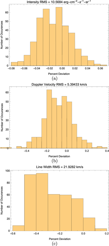
Figure 6. The differences pixel-by-pixel between the original parameter values and the reconstructed parameter values are shown. Each difference is normalized to the original and the fractional difference that results for each pixel is displayed as a distribution. The rms difference in physical units is also shown.
Download figure:
Standard image High-resolution image4.2. Effect of Spectral Dispersion
We can evaluate the effect of spectral dispersion by fixing the S/N at 50 and vary the spectral plate scale in the range from 20 to 40 mÅ/pixel. In each case the input images were the same. Reconstruction of the line fit parameters was obtained and the rms error for each case was calculated. The results are shown in Figure 7.

Figure 7. The fidelity of the reconstructions do not show significant variation for dispersion scale variations between 20 and 40 mÅ/pixel. The rms error is expressed in  for the integrated line intensity, and in km s−1 for the Doppler velocity and the line width.
Download figure:
Standard image High-resolution imageWe find that the accuracy of reconstruction is not strongly dependent on the spectral plate scale for the range that we were able to simulate. Even though an optimum value is expected from physical arguments, we were not able to demonstrate it in this simulation. A more detailed model (Oktem et al. 2014) for pixel sampling the image would allow the range of validity for the dispersion scale to be extended. Typically, spectrometers like Hinode/EIS have higher dispersions with spectral plate scales of order 20–30 mÅ/pixel, these simulations show that much larger dispersion scales could be used. This would result in increased spectral coverage, and smaller instruments with similar performance.
4.3. Effect of Noise
To evaluate the effect of S/N, we fix the dispersion scale at 30 mÅ per pixel. We vary the S/N in the three spectral order images. The value of the S/N used here is defined as the S/N of the pixel which has a value equal to 90% of the maximum pixel in the image. This value is scaled to pixels with lower and higher values as appropriate. Three values of the S/N were considered, 30, 50, and 100. Results are shown in Figure 8.

Figure 8. Accuracy of the reconstructed parameter values increases with increased S/N as expected. Units are the same as in Figure 7.
Download figure:
Standard image High-resolution image
We find, as expected, that as the S/N increases the rms errors decrease. For an S/N greater than 50, the rms error is similar to the errors obtained from fitting in a slit spectrograph. From this we infer that the addition of more complicated observing situations, like overlapping neighboring emission lines, will still allow a solution with errors in the Doppler shift ≤10 km s−1, and errors in the intensity and line width of ≤15 km s−1. Verification of this expectation is left for future work.
5. Discussion and Conclusions
In this paper we have shown that reconstruction can produce results that are accurate enough to provide useful spectral information, provided that multiple orders, say 0 and ±1, can be observed simultaneously. The reconstruction accuracy of the line fit parameters is of the same order as the line fitting accuracy of current state-of-the-art narrow-slit spectrographs like Hinode/EIS.
The results presented in this paper should be considered only a lower limit to the possibilities of the optimization method. There are two reasons for this. First, the penalty function used in this model is only one of many that could be constructed. Experimentation to find the most effective penalty function for a variety of solar scenes is needed, and will result in lower reconstruction errors. Second, the line fit parameters obtained from the Hinode/EIS rasters show small pixel-to-pixel variations. Analysis shows that the values of the line fit parameters in adjacent pixels are partially correlated. We expect that features on the Sun are much smaller than those resolved by EIS, and that if they were resolved the correlation between pixels would be reduced, increasing the pixel-to-pixel variation. The method presented here works best when there are gradients of the parameters, so one would expect that the fidelity of the reconstruction would increase.
The accuracy of the reconstruction is not strongly dependent on the spectral dispersion for the range of dispersions considered in this paper. This is likely a characteristic of some combination of the reconstruction method and the properties of the original source image. Further analysis with more detailed pixel sampling methods and other solar data sets will be required to evaluate the relative contributions.
The reconstruction method presented here allows the determination of optimal instrument design and operational characteristics like spectral dispersion and S/N for the first time. These characteristics can then be tuned for the scientific objectives of the instrument. This is an important point when specifying an instrument when resources such as mass, power, and volume are constrained. Estimation-theoretic techniques (Oktem et al. 2013) can also be utilized for the determination of the optimal design.
Although the method is promising, there are several issues that remain to be evaluated. Potentially the most significant is the effect of overlapping spectral lines. This issue can be minimized by choosing the proper spectral range, but in general can never be completely eliminated. The most promising spectral ranges will contain nearly isolated spectral lines, with overlapping only by much fainter lines. Future work will center on the simulation of this situation.
We thank the referee for helpful comments that have improved this paper. F. S. O. acknowledges the hospitality and support received as a Visiting Postdoctoral Researcher at the Catholic University of America and NASA Goddard Space Flight Center, Heliophysics Division, where some of this work was performed. F. K. acknowledges the NASA grant 80NSSC18M0052 of the Small Spacecraft Technology Program. This work has also been partially supported by the NASA grant NNX12AL74H.