


Abstract
The polytropic behavior of space plasmas defines a power law between the plasma moments during the transition of the plasma from one state to another under constant specific heat. Knowledge of the polytropic index—the power-law exponent—is essential for understanding the dynamics of plasma particles, while a full kinetic description can be established by the study of the velocity distribution of plasma particles. The particle velocities of collisionless space plasmas, such as the solar wind, follow the kappa distribution function. The kappa index, the parameter that labels and governs these distributions, is an independent variable that describes the state of plasmas and is required for a complete description of the plasma properties. Previous studies showed and demonstrated how the kappa and polytropic indices are related to each other in the presence of potential energy, and their relationship also depends on the potential degrees of freedom. This paper extends these analyses and derives the kappa and polytropic indices of the solar wind proton plasmas using Wind observations during the last two solar cycles. We examine and show the systematic long-term correlation between these indices, the magnetic field strength, and the solar activity.
Export citation and abstract BibTeX RIS
1. Introduction
The polytropic behavior is a macroscopic relationship between plasma moments that describes the transition of a plasma from one state to another under constant specific heat (e.g., Parker 1963; Chandrasekhar 1967):

where the exponent γ constitutes the polytropic index, which is characteristic for individual plasma streamlines and it may vary for different plasma species, within different plasma regimes, and/or with time (for example, see: Sittler & Scudder 1980; Osherovich et al. 1993, 1998, 1999; Newbury et al. 1997; Borovsky et al. 1998; Sittler & Burlaga 1998; Kartalev et al. 2006; Liu et al. 2006, Nicolaou et al. 2014a; Nicolaou & Livadiotis 2017; Livadiotis 2016; Dialynas et al. 2018; Prasad et al. 2018). The studies of the long-term behavior of the solar wind proton polytropic index (e.g., Nicolaou et al. 2014a; Livadiotis 2018a), calculated an average value γ ∼ 1.8, and it is found to be independent of the solar wind speed (Totten & Freeman 1995; Livadiotis 2018a). (Note: the symbols used in this study are defined in Table 1.)
Table 1. Symbols for the Physical Quantities Used in This Paper
| Symbol | Physical quantity |
|---|---|
| mp | proton mass |
| kB | Boltzmann constant |
| n | number density |
| ρ = nmp | mass density |
| VSW | bulk speed |
u
|
thermal speed derived from statistical moments |
u
|
thermal speed derived from fitting |

|
temperature in terms of energy |
| P = nkBT | thermal Pressure |
| B | magnetic field strength |
| σi | one-sigma error of the parameter i |
| δi | standard error of the parameter i |
| d | degrees of freedom |
| γ | polytropic index |
| ν = 1/(γ-1) | secondary notation of a polytropic index |
| κ | standard kappa index |

|
invariant kappa index for d |

|
potential degrees of freedom |
| dr | dimensionality |
| Sn | sunspot number |
| r | heliocentric distance |
| Φ | potential |
Download table as: ASCIITypeset image
Recently, it has been shown that the polytropic relationship is equivalent to the formulation of kappa distributions (Livadiotis 2019a). It was specifically shown that not only the kappa distributions can lead to the polytropic behavior, but the reverse derivation is also true, namely, the polytropic behavior act as a mechanism that produces kappa distributions.
Several studies have shown that the velocity and energy distributions of space plasmas follow the kappa distribution function (e.g., see: the book Livadiotis 2017; the reviews Pierrard & Lazar 2010; Livadiotis & McComas 2013a; Livadiotis 2015a, and references therein). While Maxwell–Boltzmann distributions describe particle systems residing in the stationary state of the classical thermal equilibrium, kappa distributions describe particle systems residing in stationary states of a generalized thermal equilibrium. Specifically, it was shown that kappa distributions are consistent with (i) statistical mechanics, as they maximize entropy under the constraints of a canonical ensemble (Treumann 1999; Leubner 2002; Milovanov & Zelenyi 2002; Livadiotis & McComas 2009); and (ii) thermodynamics, namely, particle systems exchanging heat and reaching thermodynamic equilibrium are always stabilized into a kappa distribution (Livadiotis 2018c).
The kappa index, the parameter that labels and governs kappa distributions, indicates how far the system resides from the classical thermal equilibrium (e.g., Livadiotis & McComas 2009, 2010, 2013a; Livadiotis 2015a), while attaining the physical meaning of an intensive parameter consistent with thermodynamics (Livadiotis 2018c). It characterizes the stationary state of the plasma and determines the correlation of the energies of two different plasma particles (Livadiotis & McComas 2011). Therefore, the determination of the kappa index is crucial for the complete description of the plasma kinetics and thermodynamics, and for understanding the physical mechanisms and processes taking place in plasma systems.
Given the strong connection of the kappa index with the thermodynamic characterization of plasmas, it is not unusual for it to be measured within a broad range of values within different plasma regimes, to exhibit large temporal variations, and/or to be correlated with other plasma parameters. Indeed, the kappa index has been extensively studied for numerous space plasmas and found to vary significantly within different plasma regimes; e.g., the solar wind (e.g., Collier et al. 1996; Mann et al. 2002; Zouganelis et al. 2004; Maksimovic et al. 2005; Marsch 2006; Yoon et al. 2006; Pierrard & Lazar 2010), across interplanetary shocks (Wilson et al. 2019), planetary magnetospheres (e.g., Sckopke et al. 1981; Hapgood & Bryant 1992; Mauk et al. 2004; Dialynas et al. 2009, 2018; Ogasawara et al. 2013; Nicolaou et al. 2014b), the outer heliosphere and the inner heliosheath (e.g., Decker & Krimigis 2003; Decker et al. 2005; Zank et al. 2010; Livadiotis et al. 2011, 2012, 2013; Livadiotis & McComas 2012).
Both the polytropic and kappa indices characterize local processes; they are constant along individual plasma streamlines, but they may vary within different plasma regimes and/or time. A strong correlation between these indices has been shown to exist for the solar wind proton plasma near 1 au (e.g., Ogasawara et al. 2017; Livadiotis 2018b; Livadiotis et al. 2018) (see Figure 1). The exact relationship between these indices also involves the potential degrees of freedom d (Livadiotis 2018b, 2019a, 2019b, 2019c):

where we consider a negative attractive central potential,  ,
,  . We used the notation of the invariant kappa index κ0. The standard kappa index κ was shown to be dependent on the degrees of freedom (d.o.f.) d,
  , so that the difference
  is invariant under variations of d.o.f.; for d = 3, this is written as
  (for more details, see Livadiotis & McComas 2011; Livadiotis 2015c).
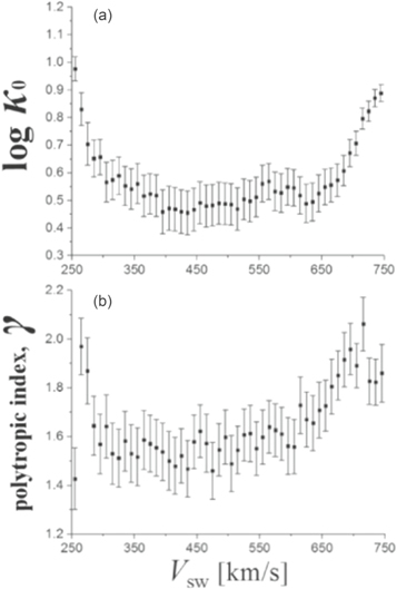
Figure 1. Mean values and their standard errors of (a) log κ0 and (b) γ, for the solar wind proton plasma near 1 au, plotted against the solar wind flow speed VSW. (Adapted from Livadiotis et al. 2018.)
Download figure:
Standard image High-resolution imageRecently, we used the positional kappa distribution in the presence of potential energy in order to examine the relationship between the polytropic and kappa indices of the solar wind protons (Livadiotis 2018b). Therefore, a systematic data analysis for deriving the polytropic and kappa indices and applying them to their linear relationship shown in Equation (2), may lead to determining the potential degrees of freedom, and thus to understanding the nature of the present potential.
In this paper, we carry out the first systematic, long-term study of the relation between the polytropic and kappa indices, in order to investigate the nature of the potential present in the solar wind plasma near 1 au and over the last two solar cycles. In Section 2 we describe the Wind data set that we use in this study. We explain how the solar wind proton bulk parameters are derived and show characteristic time series of the parameters we use through our analysis. In Section 3 we present the data analysis followed in order to derive the polytropic and kappa indices; then, we show the method to quantify the relationship between these two indices. In Section 4 we show the results of the derived indices for each year from 1995 to 2017 and we describe their characteristic features. We discuss our results in Section 5; specifically, we show the annual averages of the key parameters as a function of time, and investigate the correlations among them, the solar activity and the interplanetary magnetic field strength; we also examine the functional form of the potential energy based on our findings. In Section 6, we summarize our basic conclusions.
2. Data
We use ∼92 s resolution Wind measurements of solar wind protons and magnetic field strength from 1995 to 2017. The Wind/SWE experiment (Ogilvie et al. 1995) measures the plasma particles and determines their velocity distribution function. The proton bulk parameters n, VSW, and uth are derived by (i) calculating the statistical moments of the distribution function, and (ii) fitting a bi-Maxwellian distribution to the observations (Kasper 2003). The fitting also derives the 1σ error of the plasma parameters and the χ2; these provide a measure of the goodness of the fitting. The Wind/MFI experiment (Lepping et al. 1995) measures the magnetic field strength B, averaged over the plasma data resolution (92s). (All data sets can be found at https://cdaweb.gsfc.nasa.gov/index.html/.)
In Figure 2, we show the solar wind plasma bulk parameters and the magnetic field as measured for 1995, and in Figure 3, we show the dynamic, thermal, and magnetic pressure calculated for the same time period. The plasma temperature is calculated from the thermal speed (Table 1). We also use the annual sunspot number Sn from the World Data Center SILSO, Royal Observatory of Belgium, Brussels.

Figure 2. 92 s resolution solar wind plasma and magnetic field strength measurements by Wind/SWE and Wind/MFI, respectively, during 1995.
Download figure:
Standard image High-resolution image
Figure 3. Solar wind pressure terms calculated using Wind plasma and magnetic field measurements (shown in Figure 2); From top to bottom: dynamic pressure, thermal pressure for uth,m (Tm), thermal pressure for uth,f (Tf), magnetic pressure, and total pressure (using average temperature (Tm + Tf)/2).
Download figure:
Standard image High-resolution image3. Methodology
3.1. Subintervals Selection
The polytropic relationship applies along the same streamline plasma flow. Hence, for the calculation of γ, we need to analyze subintervals obtained within the same streamline. The analyzed subintervals obtained from a single spacecraft (S/C) should be sufficiently short in order to minimize the possibility of mixing measurements of different streamlines. Following previous studies (e.g., Kartalev et al. 2006; Nicolaou et al. 2014a; Livadiotis & Desai 2016; Livadiotis 2018a; Elliot et al. 2019), we analyze every 5 consecutive Wind measurements, which cover ∼8 minutes if there are no time gaps between them. In order to exclude subintervals with large time gaps we reject any subinterval that covers a time period larger than 10 minutes.
3.2. Calculation of the Polytropic Index γ
Taking the logarithm of Equation (1), we have

where the constant is different for different streamlines. We use orthogonal regression to calculate γ and σγ from the slope of  , within each subinterval of 5 consecutive measurements. The left panel of Figure 4 shows the fitting of Equation (3) to the density–temperature data within the subinterval obtained in DOY: 1995 January 4, from ∼10:20 to ∼10:28 UT. For the specific example, the slope in the
  diagram is 0.58 ± 0.04, thus, γ = 1.58 ± 0.04.

Figure 4. Regression for estimating the polytropic and kappa indices for the sample data subinterval obtained on the DOY 1995 January 4 between ∼10:20 and ∼10:28UT. (Left) The linear relationship between log T and log n indicates a streamline with a nearly adiabatic plasma (γ = 1.58 ± 0.04). (Middle) Fitting of Equation (4) to the data within the same subinterval; the fitted line is forced to pass from the origin and its slope indicates κ0 = 7.26 ± 0.08. (Right) The Bernoulli integral is estimated for each point of the selected subinterval (black dots), while the red lines indicate ±10% deviation of the mean value; apparently, the standard deviation of the mean value is quite smaller than this deviation; the constancy of the Bernoulli integral enhances the possibility that the measurements correspond to the same streamline, validating the estimation of the indices γ and κ0.
Download figure:
Standard image High-resolution image3.3. Calculation of the Invariant Kappa Index κ0
As explained in Livadiotis et al. (2018), and based on the work of Nicolaou & Livadiotis (2016), the invariant kappa index, for a 3D kappa distribution function, can be calculated by combining uth,m and uth,f:
In Equation (4), we assume that the bi-Maxwellian fitting to the observed proton distributions underestimates the actual thermal speed of the plasma because the fitted model does not account for the higher energy "tails" of the distribution function (for more details, see: Nicolaou & Livadiotis 2016; Livadiotis 2018b). This underestimation is reflected in the values of thermal speed and pressure, samples of which are plotted in Figures 2 and 3; uth,m is higher than uth,f and the thermal pressure calculated for uth,m is higher than the thermal pressure calculated for uth,f.
We use orthogonal regression to calculate κ0 and σκ from the slope of the diagram of  plotted against
  . The kappa index is estimated along with the polytropic index for each selected subinterval (discussed in Section 3.1). Note that according to Equation (4), the fitted line passes from the origin (thus we apply linear regression with the intercept fixed to zero). In the middle panel of Figure 4 we show an example of this fitting to the subinterval obtained in 1995 January 4 between ∼10:20 and ∼10:28 UT. For the specific subinterval, our analysis derives κ0 = 7.26 ± 0.08.
3.4. Data Selection and Filtering
3.4.1. Error of Plasma Parameters
We exclude data points with large errors, in order to minimize the propagated error in the derived parameters. Similarly to Livadiotis (2018b), we analyze data points with relative density error  and relative temperature error
  smaller than 30%. In addition, we reject subintervals that include data point(s) for which the χ2 value is larger than 5. Finally, we reject subintervals for which the calculated
  from linear regression σκ or σγ is larger than 1.
3.4.2. Bernoulli Integral
In order to enhance the possibility that the analyzed subintervals correspond to individual streamlines where the polytropic relation is valid, we analyze only subintervals with quasi-constant energy of the proton plasma, that is, the Bernoulli integral (Kartalev et al. 2006; Nicolaou et al. 2014a; Pang et al. 2015, 2016; Livadiotis 2018a, 2018b; Park et al. 2019). For the plasma near 1 au, the Bernoulli integral can be estimated from the plasma parameters as (e.g., Livadiotis 2016):

where P/ρ = kBT/mp = 1/2 ·  .
.
In the presented analysis, we first calculate the Bernoulli integral for each subinterval (five consecutive data points) using Equation 5(a) if  , and Equation 5(b) if
  . We then reject subintervals for which the standard deviation of the Bernoulli integral is larger than 10% of its average value. The right panel of Figure 4 shows the Bernoulli integral calculated for the subinterval obtained in 1995 January 4 from ∼10:20 and ∼10:28. The red dashed lines in the plot correspond to the mean value ±10%. The nearly constant Bernoulli integral within the specific subinterval enhances the possibility that the analyzed plasma belongs to the same streamline.
4. Results
4.1. Dependence of the Polytropic and Kappa Indices on the Solar Wind Speed
First, we examine the dependence of γ and κ0 on the solar wind speed VSW, and then determine the relationship between the two indices. For each year, we generate the 2D histograms of γ and log κ0 as a function of VSW (similarly to Livadiotis & Desai 2016; Livadiotis 2018a). Figure 5 shows such a histogram for 1997, while Figure 6 shows the specific panels for the years from 1995 to 2017. For each year, we show (left) the non-normalized and (right) normalized occurrence of (top) γ and (bottom) log κ0.

Figure 5. (Left) Non-normalized and (right) normalized 2D histograms of (top) γ and (bottom) log κ0 as a function of VSW for the year 1997. The white lines indicate the corresponding average values per VSW-bin.
Download figure:
Standard image High-resolution image
Figure 6. Annual (left) non-normalized and (right) normalized 2D histograms of (top) γ and (bottom) log κ0, plotted as a function of VSW, for the years from 1995 to 2017. The white lines indicate the corresponding average values per VSW-bin.
Download figure:
Standard image High-resolution imageFor each velocity bin (column), we calculate the mean values of γ, log κ0 (white lines in Figures 5 and 6) and their standard errors δγ and δlog κ0, which we use to calculate the mean values of the secondary polytropic index  and the kappa index
  , as well as their propagation errors δν and δκ0, respectively. Figure 7 shows the estimated mean values of ν and log κ0, as a function of the solar wind speed VSW for each year from 1995 to 2017.
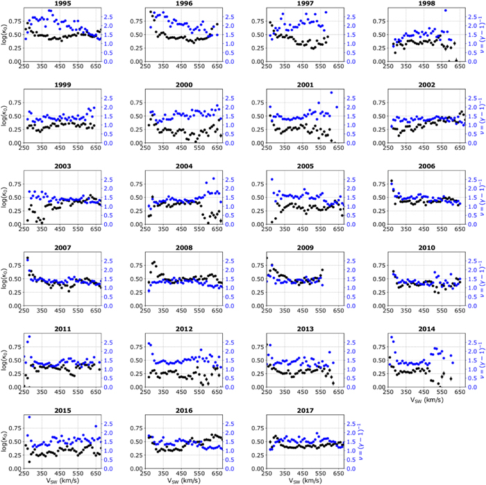
Figure 7. Average (per VSW-bin) of the polytropic index ν and the logarithm of the kappa index κ0 for each year from 1995 to 2017.
Download figure:
Standard image High-resolution image4.2. Polytropic-Kappa Linear Relationship and Potential Degrees of Freedom
According to Equation (2), the secondary polytropic index ν is linearly related to the kappa index κ0, with the slope equal to −1, and y-axis intercept given by:

For each year, we select the data points that follow the expected linear relation. The selection is based on the χ2 optimization between the selected data points and the theoretical line in Equation (2). Our analysis excludes data points with κ0 larger than 4.5, which is the theoretical limit of kappa indices for 3D kappa distributions describing both the kinetic and potential energy with  (Livadiotis 2015b). We calculate the average y-intercept
  from the N selected data points (κ0i, νi), as follows:
where  and
and  . The standard error of
  is
is

where  is the propagation error:
 is the statistical error:
Finally, we calculate the potential degrees of freedom:

Figure 8 shows the indices ν and κ0 (averaged per VSW-bin) plotted as a function of the solar wind speed VSW for the annual interval in 1997; it also shows κ0 plotted against ν, by canceling VSW. The blue data points (νi, κ0i,) are fitted with Equation (2) (dashed line) in order to estimate the value of the potential d.o.f.,  . The analysis is completed for each year from 1995–2017, in order to examine the long-term variation of
  over the last two solar cycles (see also Table 2). In Figure 9, we show the panels of κ0 plotted against ν (similar to that in the top right panel of Figure 8), for all the years from 1995 to 2017.
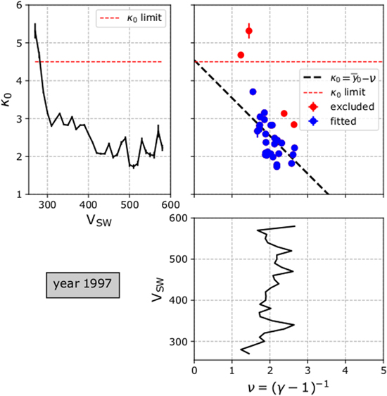
Figure 8. (Top left) κ0 and (bottom) ν indices plotted as a function of VSW for 1997. (Top right) κ0 plotted as a function of ν. Data points lying above the theoretical limit κ0 = 4.5 (red dashed line) are excluded from this analysis (see the text). The data points (blue dots) follow the fitted linear relationship shown in Equation (2).
Download figure:
Standard image High-resolution image
Figure 9. Plots of κ0 as a function of ν for each year from 1995 to 2017 (in the same format as in the top right panel of Figure 8). Errors of ν are not shown, for clarity.
Download figure:
Standard image High-resolution imageTable 2. Annual Means of Polytropic and Kappa Indices, and the Related Potential d.o.f, for 1995–2017
| Year |

|

|
σγ |

|
σlog κ0 |

|
σκ0 |

|

|
|---|---|---|---|---|---|---|---|---|---|
| 1995 | 2.24 | 1.45 | 1.09 | 0.48 | 0.29 | 3.00 | 2.00 | 5.89 | 0.05 |
| 1996 | 2.25 | 1.45 | 1.04 | 0.46 | 0.25 | 2.91 | 1.70 | n/a | n/a |
| 1997 | 1.98 | 1.50 | 1.11 | 0.43 | 0.32 | 2.72 | 2.02 | 5.57 | 0.06 |
| 1998 | 1.46 | 1.69 | 1.07 | 0.34 | 0.35 | 2.18 | 1.76 | 4.75 | 0.04 |
| 1999 | 1.38 | 1.73 | 1.01 | 0.31 | 0.36 | 2.03 | 1.69 | 4.53 | 0.04 |
| 2000 | 1.45 | 1.69 | 1.03 | 0.22 | 0.38 | 1.66 | 1.43 | 3.94 | 0.03 |
| 2001 | 1.43 | 1.70 | 1.05 | 0.25 | 0.39 | 1.77 | 1.60 | 4.21 | 0.04 |
| 2002 | 1.30 | 1.77 | 1.02 | 0.30 | 0.33 | 1.98 | 1.52 | n/a | n/a |
| 2003 | 1.38 | 1.73 | 0.97 | 0.36 | 0.32 | 2.31 | 1.70 | 4.78 | 0.05 |
| 2004 | 1.35 | 1.74 | 1.02 | 0.36 | 0.33 | 2.30 | 1.75 | 4.70 | 0.03 |
| 2005 | 1.56 | 1.64 | 1.05 | 0.31 | 0.34 | 2.04 | 1.58 | 4.72 | 0.04 |
| 2006 | 1.48 | 1.68 | 1.03 | 0.43 | 0.28 | 2.68 | 1.72 | 5.07 | 0.03 |
| 2007 | 1.40 | 1.72 | 1.00 | 0.44 | 0.28 | 2.78 | 1.77 | n/a | n/a |
| 2008 | 1.32 | 1.76 | 0.95 | 0.52 | 0.28 | 3.32 | 2.17 | 5.51 | 0.05 |
| 2009 | 1.38 | 1.73 | 1.01 | 0.53 | 0.29 | 3.41 | 2.30 | n/a | n/a |
| 2010 | 1.34 | 1.74 | 1.03 | 0.40 | 0.32 | 2.52 | 1.87 | 4.82 | 0.04 |
| 2011 | 1.32 | 1.76 | 1.03 | 0.35 | 0.34 | 2.24 | 1.73 | 4.65 | 0.03 |
| 2012 | 1.43 | 1.70 | 1.06 | 0.25 | 0.35 | 1.76 | 1.43 | 4.19 | 0.04 |
| 2013 | 1.40 | 1.71 | 1.08 | 0.28 | 0.35 | 1.89 | 1.51 | 4.30 | 0.03 |
| 2014 | 1.40 | 1.71 | 1.05 | 0.28 | 0.34 | 1.91 | 1.47 | 4.26 | 0.03 |
| 2015 | 1.46 | 1.68 | 1.02 | 0.30 | 0.31 | 1.99 | 1.43 | 5.16 | 0.02 |
| 2016 | 1.44 | 1.70 | 1.02 | 0.39 | 0.30 | 2.47 | 1.69 | 5.38 | 0.04 |
| 2017 | 1.57 | 1.64 | 1.02 | 0.42 | 0.27 | 2.63 | 1.66 | 5.23 | 0.03 |
Download table as: ASCIITypeset image
4.3. Description of the Results
The occurrences of γ and log κ0 as a function of VSW (Figures 5 and 6) show that γ ranges between −2.5 and 5 and log κ0 ranges between −1 and 1, but they mostly lie around their mean values, that is, ∼1.68 and ∼0.37, respectively. The average γ and log κ0 (per VSW bin, white lines in Figures 5 and 6) do not exhibit any characteristic or systematic variation with VSW. The standard error of both indices is of the same order for the entire solar wind speed range (see also Figure 1). We note that the standard error increases with the spread of the values around their mean and decreases when increasing the amount of samples within each VSW bin. Therefore, as the majority of the data reside in the intermediate speeds, our result indicates that the spread of γ and κ0 is greater within that speed range.
The γ values are roughly symmetrically distributed; log κ0 values occasionally exhibit asymmetric occurrences with "tails" toward the lower log κ0 values. We observe these "tails" to be more pronounced during years with stronger solar activity. For instance, in the years 1995–1997 and 2007–2009, corresponding to minimum solar activity periods, the occurrence of log κ0 does not extend significantly below zero. On the other hand, in the years 2000–2002 and 2012–2014, corresponding to maximum solar activity, the occurrence exhibits tails extending to ∼−1. These tails shift the average log κ0 (white line on top of the occurrence plot) toward lower values.
Figure 5, shows the occurrences of the polytropic and kappa indices as a function of the solar wind speed for 1997. The average log κ0 is higher for lower speeds, VSW < 300 km s−1, whichmay be caused by less reliable measurements that characterize these speeds; for higher speeds and a wider range of speeds log κ0 almost flattens, while it slightly increases for the fast solar wind (VSW > 550 km s−1). The behavior of the polytropic and kappa indices as a function of VSW is slightly different for different years of the last two solar cycles (Figure 6).
Figure 7 shows the mean values of ν and log κ0 as a function of VSW, for each year between 1995 and 2017. Interestingly, while there is no systematic variation of both indices as a function of VSW, most of the time, the two indices are anti-correlated, as expected from theory (Livadiotis 2017, 2018b, 2019a, 2019b, 2019c). For instance, in 1997, ν ∼ 1.5 within the low speed range (VSW < 300 km s−1), reaches a maximum value ν ∼ 2.5 in the intermediate speed range (450 km s−1 < VSW < 550 km s−1) and drops again down to ν ∼ 1.5 as the speed increases (VSW > 550 km s−1). Within the same year, log κ0 follows an opposite trend; log κ0 ∼ 0.5 within the low speed range (VSW < 300 km s−1), reaches a minimum value log κ0 ∼ 0.25 in the intermediate speed range (450 km s−1 < VSW < 550 km s−1), and increases again to log κ0 ∼ 0.5 as the speed increases (VSW > 550 km s−1). In another characteristic example, in 2004, the two indices exhibit a different behavior as a function VSW but similar to 1997, they are anti-correlated. For this specific year, ν ∼ 1 in the low speed range (VSW < 300 km s−1) and ∼2 in the high speed range (VSW > 500 km s−1), exhibiting a local maximum (ν ∼ 1.5) for VSW ∼ 400 km s−1 and a local minimum (ν ∼ 1.3) for VSW ∼ 500 km s−1. In the same year, log κ0 ranges between 0.5 and 0, with a global minimum (log κ0 ∼ 0.3) at VSW ∼ 400 km s−1 and a local maximum (logκ0 ∼ 0.4) at VSW ∼ 500 km s−1.
Although we observe anti-correlation between the values of ν and κ0 in most of the annual intervals, there are examples in which the two indices do not exhibit any systematic correlation. We identify these cases in years 2002, 2007, and 2009. Interestingly, we also observe that in 1996, the two indices are positively correlated. Within this year, ν and log κ0 exhibit similar behavior within a wide range of VSW. Specifically, for VSW between 350 km s−1 and 500 km s−1, both indices decrease; ν drops from a local maximum ν ∼ 2.5, to a local minimum ν ∼ 1.5, while log κ0 decreases from local maximum log κ0 ∼ 0.6, to a local minimum log κ0 ∼ 0.35. The linear relation of Equation (2) is not applicable to any of these annual intervals (see also Figure 9). We speculate that during these annual intervals there is more than one potential affecting the distribution function of the particles. In such a case, we need to use a superposition of potentials to describe the observed relationship, which is not the scope of this current work.
We fit ν and κ0 with Equation (2), within each of the annual intervals that the two indices are anti-correlated (19 out of the 23 annual intervals) in order to determine the y-intercept  , and the potential degrees of freedom
  . In Figure 8, we show ν and κ0 as a function VSW and ν as a function of κ0 for the year 1997. In this typical example, we fit the majority of the data points with the linear model of Equation (2) and we calculate
  , therefore,
  . In Figure 9 we show ν as a function of κ0 for each year from 1995 to 2017. Although there is a clear scattering of the data points, probably due to the turbulent nature and the multiple structures within the solar wind, the linear relationship between the polytropic and kappa indices can be statistically identified in most of the annual subintervals.
5. Discussion
5.1. Long-term Behavior of Polytropic and Kappa Indices and Potential Degrees of Freedom
We investigate the annual averages of the key parameters as a function of time, for the last two solar cycles. Table 2 shows the annual averages of the polytropic index  and
and  , the logarithm of the invariant kappa index
  , the invariant kappa index
  , the potential degrees of freedom
  , and their errors, as calculated for each year from 1995 to 2017. For the years in which the linear model does not apply (that is the cases of the four years mentioned above, i.e., 1996, 2002, 2007, and 2009), we do not derive
  and
and  (listed as n/a in Table 2). Figure 10 shows the time series of the calculated average parameters along with the annual average sunspot number Sn and the interplanetary magnetic field strength B. We identify the following characteristics in the long-term behavior of the parameters:
- 1.The annual average
 and are correlated with each other, while both these parameters are anti-correlated with the solar activity. From 1995 to 2000, both and decrease monotonically as Sn increases. During the solar maximum in 2000, and reach their minimum values, ∼0.2 and ∼4, respectively. During the decay phase of the 23rd solar cycle, both and increase; during the solar minimum in 2008–2009, log κ0 reaches a maximum value ∼0.5 and reaches a local maximum ∼5.5. During the ascending phase of the 24th solar cycle between 2009 and 2012, both and drop systematically and reach local minima in 2012, before they increase again.
 - 2.The annual average polytropic index exhibits weak correlation with the solar activity. For the first three years, the plasma is sub-adiabatic, with , with a slide increase in 1997, as . From 1998 until 2017, the plasma is nearly adiabatic with ranging between 1.65 and 1.8. The results of this study do not precisely follow the characteristic long-term behavior of and its anti-correlation with the solar activity shown by Nicolaou et al. (2014a). The differences may be caused by the different number of data points per subinterval and/or by the different data sets and processing, as Nicolaou et al. (2014a) used timeshifted, cross-calibrated data sets of plasma parameters, measured by different S/C and processed with different time resolutions.


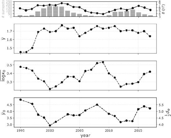
Figure 10. (From top to bottom) Time series of Sn (gray, left y-axis) and B (black, right y-axis), annual averages  ,
,  , and y-intersect
  (left y-axis) that corresponds to the potential d.o.f,
  (right y-axis). We observe that
  and
and  are correlated, while both parameters are anti-correlated with the solar activity. The polytropic index shows weaker correlation with the solar activity.
Download figure:
Standard image High-resolution image5.2. Correlation of the Potential d.o.f. with Solar Activity
We further quantify the relation between  and Sn. We seek a power-law function that relates the two parameters using the fitting method based on the correlation coefficient maximization (Livadiotis & McComas 2013b). We specifically search for the positive exponent p for which the absolute correlation coefficient between
  and
and  is maximized. Because
  and
and  are anti-correlated, we optimize the exponent p for the minimum Pearson correlation coefficient value. We find that the minimum correlation (Pearson coefficient −0.82) is achieved for p ∼ 0.6 (Figure 11, left). We achieve an approximate fit (Figure 11, right) with

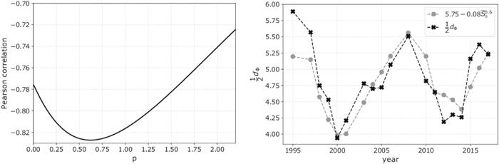
Figure 11. (Left) The (Pearson) correlation coefficient between the time series of  and
and  as a function of the exponent p. The strongest anti-correlation (Pearson coefficient <−0.82) is calculated for p ∼ 0.6. (Right) The time series of
  (black) and the
  (gray) are approximately fitted.
Download figure:
Standard image High-resolution image5.3. Evidence of a Long-term Relationship between Polytropic and Kappa Indices
We examine 23 annual intervals, from 1995 to 2017, to investigate the long-term behavior of the polytropic  and kappa κ0 indices, and quantify the linear relationship between them (averaged in each solar wind speed bin) over the last two solar cycles. In 19 of the 23 examined intervals (∼83%) we determine a significant amount of data points that are linearly correlated. The analysis of these intervals derives the potential d.o.f.,
  . This may be caused by the fact that the annually based data analysis is not sensitive for the various solar wind structures, thus we were averaging features for which the relationship between the two indices is different—for reasons that are not fully understood at the moment. A deviation from the theoretical model in Equation (2) may be expected if more than one potential is acting on the plasma particles within the specific intervals. Such intervals could be analyzed in future studies with finer resolutions, in order to resolve the existing potentials. Moreover, different solar wind structures such as magnetic clouds, CMEs, and CIRs may introduce scattering of the data points around the theoretical expectation. Also, the presence of enhanced turbulence can introduce additional data-point scattering and prevent the accurate determination of the potential d.o.f. Indeed, the anti-correlation is not persistently strong within all the analyzed annual intervals and the whole range of VSW, nonetheless the result still constitutes strong evidence of the specific correlation, verifying the results and the theoretical expectations (Livadiotis 2018a, 2018b, 2019a).
5.4. Distribution Function Affected by the Solar Activity
We found a clear variation of the annual  , which is correlated with the annual average
  . Both
  and
and  are anti-correlated with Sn (Figure 10). Further analysis quantifies the relationship between
  and Sn (Figure 11). The results indicate that, during periods of strong activity, the enhanced magnetic field induces stronger correlations among particles (Livadiotis et al. 2018), resulting in kappa distributions with lower κ0. This is specifically shown in Figure 12, where κ0 decreases with increasing Sn and B. In the right panel of Figure 12, we show the data points within the two solar cycles. The anti-correlation between κ0 and B is more pronounced during the 23rd solar cycle, for which κ0 drops from ∼3.5 to ∼1.5 as B increases from ∼3 nT to ∼8 nT. In addition, we observe anti-correlation between the magnetic field and the potential d.o.f.; we discuss this behavior in the next subsection.
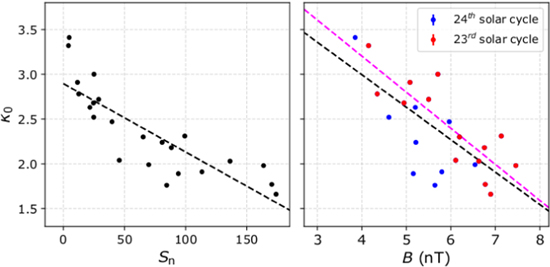
Figure 12. Kappa index κ0 plotted as a function of Sn (left) and B(right). The linear fit to data points (black dash) is shown for both panels. The dashed magenta line in the right panel corresponds to the linear fitting to the data points within the 23rd solar cycle. The result indicates that κ0 decreases with increasing Sn and B.
Download figure:
Standard image High-resolution image5.5. Implications on the Potential Energy Function
The observed d.o.f.  decreases from ∼6 during solar minimum to ∼4 during solar maximum. For the power-law central potential,

(negative  and attractive
  ), it has been shown that the d.o.f.
  can be expressed as a function of the exponent b and the potential dimensionality dr (Livadiotis 2015b, 2017, Chapters 3 and 4)

For a typical interplanetary electric field with b = 1/2 (e.g., Cuperman & Harten 1971; Lacombe et al. 2002; Livadiotis 2018b), our findings indicate that the dimensionality dr reduces from 3 during solar minimum and a weak magnetic field to 2 during solar maximum and a strong magnetic field. Table 3 shows the corresponding values of the potential dimensionality dr, for such a typical interplanetary electric potential (b = 0.5), and the annual Sn and B. Figure 13 shows dr as a function of Sn and B. The linear fitting to the data shows that during low activity and a weak interplanetary magnetic field, the interplanetary electric potential is characterized by spherical symmetry, which reduces to cylindrical symmetry during high activity and a strong interplanetary magnetic field.
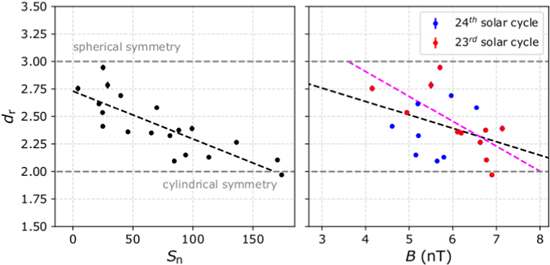
Figure 13. Dimensionality dr for a typical interplanetary potential  , as a function of Sn (left) and B(right). The linear fit to data points (black dash) is also shown for both diagrams. The dashed magenta line in the right panel corresponds to the linear fitting to the data points within the 23rd solar cycle. The results indicate that the potential dimensionality dr reduces with increasing Sn and B.
Download figure:
Standard image High-resolution imageTable 3. Annual Means of the Potential d.o.f., Space Dimensionality, and Magnetic Field for 1995–2017
| Year |

|

|
dr | δdr | B | Sn |
|---|---|---|---|---|---|---|
| 1995 | 5.89 | 0.05 | 2.95 | 0.03 | 5.71 | 25.1 |
| 1996 | n/a | n/a | n/a | n/a | 5.08 | 11.6 |
| 1997 | 5.57 | 0.06 | 2.79 | 0.03 | 5.50 | 28.9 |
| 1998 | 4.75 | 0.04 | 2.38 | 0.02 | 6.75 | 88.3 |
| 1999 | 4.53 | 0.04 | 2.27 | 0.02 | 6.63 | 136.3 |
| 2000 | 3.94 | 0.03 | 1.97 | 0.02 | 6.90 | 173.9 |
| 2001 | 4.21 | 0.04 | 2.11 | 0.02 | 6.77 | 170.4 |
| 2002 | n/a | n/a | n/a | n/a | 7.46 | 163.6 |
| 2003 | 4.78 | 0.05 | 2.39 | 0.03 | 7.13 | 99.3 |
| 2004 | 4.70 | 0.03 | 2.35 | 0.02 | 6.19 | 65.3 |
| 2005 | 4.72 | 0.04 | 2.36 | 0.02 | 6.11 | 45.8 |
| 2006 | 5.07 | 0.03 | 2.54 | 0.02 | 4.95 | 24.7 |
| 2007 | n/a | n/a | n/a | n/a | 4.35 | 12.6 |
| 2008 | 5.51 | 0.05 | 2.76 | 0.03 | 4.15 | 4.2 |
| 2009 | n/a | n/a | n/a | n/a | 3.85 | 4.8 |
| 2010 | 4.82 | 0.04 | 2.41 | 0.02 | 4.61 | 24.9 |
| 2011 | 4.65 | 0.03 | 2.33 | 0.02 | 5.21 | 80.8 |
| 2012 | 4.19 | 0.04 | 2.10 | 0.02 | 5.64 | 84.5 |
| 2013 | 4.30 | 0.03 | 2.15 | 0.02 | 5.16 | 94.0 |
| 2014 | 4.26 | 0.03 | 2.13 | 0.02 | 5.79 | 113.3 |
| 2015 | 5.16 | 0.02 | 2.58 | 0.01 | 6.54 | 69.8 |
| 2016 | 5.38 | 0.04 | 2.69 | 0.02 | 5.96 | 39.8 |
| 2017 | 5.23 | 0.03 | 2.62 | 0.02 | 5.20 | 21.7 |
Download table as: ASCIITypeset image
It is possible that both dr and b may vary with the solar activity and the interplanetary magnetic field. The diagram in Figure 14 plots the exponent b as a function of dr within the observed range of values of 1/2dΦ. In the same plot we indicate the solutions for b = 0.5, which are discussed above (intersection with the horizontal magenta), and the solutions of dr = 2 and dr = 3 (intersections with the vertical gray lines). For example, in the case of potential dimensionality fixed to dr = 3 (right gray dashed in Figure 14), our findings indicate that the exponent b would vary from 0.75 during solar maximum to 0.5 during solar minimum.

Figure 14. Potential exponent b plotted as a function of the dimensionality dr, plotted for several potential degrees of freedom  ranging from 4 (during solar maximum) to 6 (during solar minimum). Intersections with the horizontal magenta line are solutions for typical interplanetary potential with b = 0.5. Intersections with the two vertical gray lines, are solutions for dimensionalities dr = 2 and dr = 3, respectively.
Download figure:
Standard image High-resolution image
6. Conclusions
The presented paper simultaneously derived the polytropic and kappa indices of the solar wind protons over the last two solar cycles, using Wind observations. The analysis determined the long-term relationship between the two indices, from which the potential d.o.f. were derived. We examined the characteristic long-term correlation between these parameters, and how this varies with the solar activity and the interplanetary magnetic field.
In summary, in this paper we showed the following:
- 1.There is a systematic relationship between the polytropic ν = 1/(γ − 1) and kappa κ0 indices of the solar wind protons.
- 2.The kappa distribution function is affected by the solar activity and the interplanetary magnetic field. More specifically, the kappa index of the distribution function decreases with increasing solar activity and magnetic field strength.;
- 3.The potential degrees of freedom decrease with increasing solar activity and the interplanetary magnetic field strength.
- 4.The dimensionality of the particles varies with the solar activity and the magnetic field. For a typical interplanetary electric field, the dimensionality reduces from dr = 3 in solar minimum, to dr = 2 in solar maximum, meaning that particles have spatial configurations with d.o.f. close to three for weaker magnetic fields, while it flattens to a configuration of d.o.f. close to two for stronger magnetic fields.
Finally, we highlight the importance of similar studies with future S/C missions such as Solar Orbiter and Parker Solar Probe, which will provide high-resolution data at a wide range of heliocentric distances. With similar data analyses that combine plasma, magnetic, and electric field measurements from these missions, we can determine the dependence of exponent b on r, which will lead to an accurate determination of Φ(r). Additionally, we can determine Φ(r) beyond the ecliptic, by analyzing future Solar Orbiter data obtained in high-inclination orbits (>30°).
G.N. was supported by the STFC Consolidated Grant to UCL/MSSL, ST/N000722/1 and ST/S000240/01. G.L. was supported by NASA's projects NNX17AB74G and 80NSSC18K0520.