


Abstract
We report observations of small-scale swirls seen in the solar chromosphere. They are typically 2 Mm in diameter and last around 10 minutes. Using spectropolarimetric observations obtained by the CRisp Imaging Spectro-Polarimeter at the Swedish 1 m Solar Telescope, we identify and study a set of swirls in chromospheric Ca ii 8542 Å and Hα lines as well as in the photospheric Fe i line. We have three main areas of focus. First, we compare the appearance, morphology, dynamics, and associated plasma parameters between the Ca ii and Hα channels. Rotation and expansion of the chromospheric swirl pattern are explored using polar plots. Second, we explore the connection to underlying photospheric magnetic concentration (MC) dynamics. MCs are tracked using the SWAMIS tracking code. The swirl center and MC remain cospatial and share similar periods of rotation. Third, we elucidate the role swirls play in modifying chromospheric acoustic oscillations and found a temporary reduction in wave period during swirls. We use cross-correlation wavelets to examine the change in period and phase relations between different wavelengths. The physical picture that emerges is that a swirl is a flux tube that extends above an MC in a downdraft region in an intergranular lane. The rotational motion of the MC matches the chromospheric signatures. We could not determine whether a swirl is a gradual response to the photospheric motion or an actual propagating Alfvénic wave.
Export citation and abstract BibTeX RIS

Original content from this work may be used under the terms of the Creative Commons Attribution 3.0 licence. Any further distribution of this work must maintain attribution to the author(s) and the title of the work, journal citation and DOI.
1. Introduction
Solar tornadoes have been observed in the solar atmosphere for nearly a century. Their importance lies in how they act as energy channels between different layers of the solar atmosphere (Zöllner 1869; Hale 1908a, 1908b; Parker 1983; Simon & Weiss 1997; Brown et al. 2003; Wedemeyer-Böhm et al. 2012, and references therein). Tornadoes exist with different physical morphologies related to the different formation mechanisms. This study focuses on small-scale chromospheric swirls (Wedemeyer-Böhm & Rouppe van der Voort 2009) that have heights between 2 and 3 Mm and diameters between 1 and 3 Mm.
Instruments such as the CRisp Imaging Spectro-Polarimeter (CRISP; Scharmer et al. 2008) on the Swedish 1 m Solar Telescope (SST; Scharmer et al. 2003) equipped with adaptive optics have advanced to the extent that it has now become routinely possible to observe vortices on much smaller scales (≤1 Mm wide), and their evolution is close to the telescope's diffraction limit. With image reconstruction techniques, spatial resolutions can be achieved that are below the mean free path of photons, which, in the solar photosphere and chromosphere, is typically between 70 and 120 km. At such scales, one can study the evolution of photospheric granules and magnetic concentrations (MCs) lying in narrow and corrugated granular downflow lanes.
Swirls are believed to be connected with photospheric vortex flows of several megameters in size associated with granulation and located in intergranular lanes and junctions (e.g., Brandt et al. 1988; Bonet et al. 2008; Attie et al. 2009). Vortices observed by Bonet et al. (2008) in G-band images were thought to be associated with the motions of MCs lasting ≈5 minutes, similar to granular lifetimes. At the solar surface, these convective motions are driven by localized downdrafts as photons stream freely into space, rapidly cooling the atmosphere. As the angular momentum is conserved, the converging plasma spins as it approaches the center of the sink, thus forming a whirlpool-like flow. The magnetic field twists and unwinds the built-up stresses above the MCs. Numerical simulations have confirmed the formation of granular vortex flows that lead to the formation of swirling motions in vertical vortex tubes (Shelyag et al. 2011), the role of magnetic fields, and the connection between magnetic vortices and rotary motions of photospheric bright points (Kitiashvili et al. 2012).
Chromospheric plasma spirals upward, producing the observed signatures of the chromospheric swirls (Wedemeyer-Böhm & Rouppe van der Voort 2009) or "magnetic tornadoes" (Wedemeyer-Böhm et al. 2012). Wedemeyer-Böhm et al. (2012) observed chromospheric swirls in Ca ii (8542 Å). They found Doppler velocities of 4 km s−1 and evidence of an increase in swirl cross section with height, implying a "magnetic tornado." Thus, these swirls represent a highly organized structure that can transfer mass and energy into the corona, as the vortices and associated waves are able to channel the energy to the overlying solar atmosphere to dissipate as heat.
The swirls were tracked from the chromosphere to the corona using a combination of images from the SST and the Solar Dynamics Observatory (SDO; Lemen et al. 2012). Using CO5BOLD simulations, Wedemeyer-Böhm et al. (2012) have shown that swirls may provide, through the form of torsional Alfvén waves, a Poynting flux of 440 W m2 into the lower corona. As the Poynting flux required to heat the quiet-Sun corona and drive the solar wind is around of 100–300 W m−2 (Withbroe & Noyes 1977), they argued that swirls form an attractive alternative mechanism of channeling energy into the upper solar atmosphere.
We present an observational study of chromospheric swirls with three main areas of focus. First, we wish to compare the appearance, morphology, dynamics, and associated plasma parameters between the Ca ii and Hα channels. Traditionally, swirls have been observed in Ca ii only. Second, we wish to explore the connection to underlying photospheric MC dynamics. Third, we wish to elucidate the role swirls play in modifying and possibly generating chromospheric acoustic oscillations (e.g., Kitiashvili et al. 2011). The paper is organized as follows. Observations related to the swirls are described in Section 2. Section 3 discusses the analysis and results for two detailed case studies. Discussions and conclusions related to the swirls are described in Section 4.
2. Observations
2.1. Data Details
We present observations carried out between 08:07:24 and 09:05:46 UT on 2012 June 21, using the CRISP instrument on the Swedish 1 m Solar Telescope. The spatial resolution of these observations is 0 16 at 6302.0 Å and 020 at 8542 Å. The spatial sampling of the detector is 0059/pixel. The time cadence of the data is 8 s. The data were reconstructed using Multi-Object Multi-Frame Blind Deconvolution (MOMFBD; van Noort et al. 2005). The field of view (FOV) of 55'' ×55'' was centered in the quiet-Sun region, at solar-x = −31 and solar-y = 699. Using CRISP, we observed 11 line positions along the Hα line scan with increments of ±0.26 Å from the line center at 6563.0 Å up to ±1.29 Å. For the Ca ii line scan, we observed 19 line positions with increments of ±0.055 Å from the line center at 8542.0 Å up to ±0.495 Å. We obtained polarimetric observations in Fe 6302 Å at a single wavelength position at +0.043 Å from the line center. Figure 1 shows the SST FOV on an SDO-AIA 1600 channel full-disk image of the Sun. The context images for SST obtained in Hα at +1.29 Å from the line core, Ca ii 8542 Å at 0.495 Å from the line core, and Stokes-V of Fe 6302 Å are shown in subpanels (e)–(g). Reference images from SDO-AIA covering temperatures ranging between 4500 and 600,000 K are shown in subpanels (b)–(d) and (h).
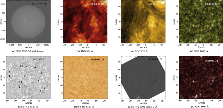
Figure 1. Quiet-Sun observations carried out on 2012 June 21. Subpanels (a) and (b) show CRISP (SST) wavelengths are represented by the panels covering wings of Ca ii 8542 Å, Hα, and Fe 6302 Å (adapted from Shetye et al. 2018). The locations of the "swirls" are indicated by numbers corresponding to them.
Download figure:
Standard image High-resolution image2.2. Details of Swirl Observations
Chromospheric swirls are difficult to identify without clear, well-developed signatures in intensity. Therefore, we have adopted a set of visual criteria for selecting candidate swirls. First, we need to observe a circular pattern in intensity, at least at one time, in the line core of Ca ii 8542.11 Å and in its wings at ±0.11 Å, as well as in the Hα line core and 0.26 Å red wing. In Hα, swirls have a more fragmented appearance than in Ca ii. Second, we require that the swirl is associated with one or more photospheric magnetic concentrations observed in Fe 6302 Å. This emphasizes the connection between photospheric and chromospheric dynamics as suggested by Wedemeyer-Böhm et al. (2012).
In our data set, we have been able to visually identify 13 candidate swirls using these criteria. Their locations are indicated on an SST context image in Figure 1. Also, further basic details are provided for all swirls in the Appendix. The observed swirls have an average diameter of 15 and lifetime of 9–10 minutes, as seen in the Ca ii wings. The lifetime is estimated based on the duration of time over which the feature can be visually tracked. These signatures are consistent with previous reports by Wedemeyer-Böhm et al. (2012). The five most promising swirl candidates are shown at a given time in the various channels in Figure 2. As we shall see, these swirls also broadly satisfy the identification criteria for a chromospheric swirl set out by Wedemeyer et al. (2013). We have constructed Doppler difference images from intensity differences at ±3.5 km s−1 from the Ca ii line core. The blue color implies upflow and the red downflow. During the appearance of swirls in the Ca ii line, we observe cospatial bright-intensity ring fragments in Hα. Such cospatial Ca ii–Hα swirl features have not been reported before.
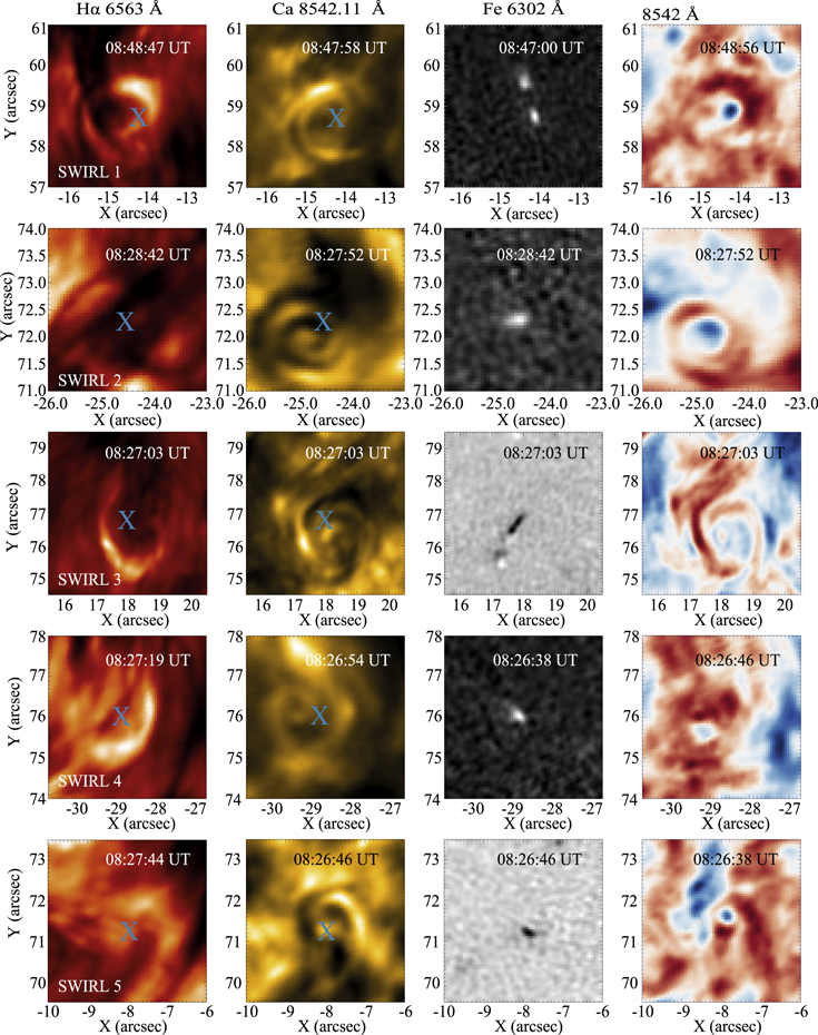
Figure 2. Snapshots in Hα 6563 Å, Ca ii 8542.11 Å, and Stokes-V of Fe 6302 Å, and Doppler difference images constructed in Ca ii 8542 Å showing selected swirling events. Blue crosses show the positions of the MCs overplotted on the Hα 6563 Å and Ca ii 8542.11 Å images. These are Swirls 1–5 from Figure 11.
Download figure:
Standard image High-resolution imageUnder the second criterion, the population of swirls can be split into two categories: five associated with multiple MCs, and eight associated with a single MC. We have chosen to present the analysis of the clearest swirl from both categories. Swirl 1 is representative of a chromospheric swirl formed above multiple MCs and is similar to Swirls 3, 8, 9, and 10. Swirl 2 is representative of a chromospheric swirl formed above a single MC and is similar to Swirls 4, 5, 6, 7, 11, 12, and 13. The time evolution of Swirls 1 and 2 is shown in Figures 3 and 4, respectively. We shall first provide an overall description of the appearance and evolution of the two swirls in the chromospheric channels and the underlying MCs in the photospheric channel. Later we shall undertake an in-depth analysis.
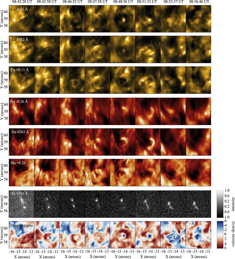
Figure 3. Evolution of Swirl 1 from 08:42 UT to 08:57 UT. The top three rows show the evolution observed in ±0.11 Å and the Ca ii 8542 line core. The next three rows show the evolution in the Hα wavelengths ±0.26 Å and Hα 6563 Å line core. The seventh row shows the evolution of MCs in Fe i 6302 Å, and the last row shows a sequence of Doppler images constructed in the Ca ii 8542 Å wings. Black crosses on the Doppler images indicate the locations of centers of the swirls when they change Doppler sign. Color bars on the right show the Doppler velocity range and intensity.
Download figure:
Standard image High-resolution image
Figure 4. Evolution of Swirl 2 from 08:18 UT to 08:34 UT. The description of the rows is the same as for Figure 3.
Download figure:
Standard image High-resolution imageSwirl 1: The evolution of Swirl 1 is shown as a set of time snapshots in the various channels in Figure 3. The swirl is visible in the chromosphere between 08:42 and 08:57 UT. At 08:46 UT, roughly 10 minutes after the appearance of the MC, a circular structure is observed first in the Ca ii +0.11 Å red wing, followed by the Ca ii line core and −0.11 Å blue wing a minute later. Around the same time, circular patterns are observed in the Hα core and ±0.26 Å wings, though partially obscured by chromospheric fibrils. The circular chromospheric pattern further develops into a swirl, as seen as a pattern of intensity enhancement that forms one or more spiral curves, or "arms." Within the curve, the intensity is reduced, which enhances the swirl pattern. It is observed to rotate around its axis, as well as expanding as it evolves. Also, in Hα there is a modulation of the overall swirl intensity with time. Overall, the swirl is visible for 15 minutes.
During the initial stage, the arms of this swirl are redshifted but the swirl center is blueshifted, as seen in the Doppler difference images in Figure 3. However, later around 08:48–08:51 UT, the Doppler signal changes sign, where the arms are now seen blueshifted and the swirl center is redshifted. We have emphasized this effect in Figure 3 by placing black crosses on the swirl centers at times of a change in Doppler sign. The chromospheric dynamics are analyzed in more detail in Sections 3.2 and 3.3.
In the photosphere, two MCs of the same polarity become visible in Fe i Stokes-V around 08:35 UT, one to the north (top MC) and one to the south (bottom MC). The bottom MC is cospatial with the chromospheric swirl, such that the swirl center tracks the MC position. The top MC moves south a distance of about 100 km toward the bottom MC. At the same time, the bottom MC has two components of motion, which may be interpreted as a rotation of the MC around an external center that itself is translating. Furthermore, the evolution of its shape is suggestive of rotation of the MC itself. These rotational motions, combined with the cospatiality, suggest that this MC lies at the footpoint of and is connected with the chromospheric swirl.
Swirl 2: the evolution of Swirl 2 is shown as a set of time snapshots in the various channels in Figure 4. The swirl is visible in the chromosphere between 08:18 UT and 08:34 UT. A circular pattern begins to appear around 08:18 UT in Ca ii. This pattern develops into a swirl similar to Swirl 1 from 08:26 UT. However, the circular pattern is not prominent in Hα. Similar to Swirl 1, Doppler difference images show a blueshifted center at the swirl with a redshifted arm, as well as a change of Doppler sign with time. Again, we have placed black crosses on the Doppler difference images to indicate a change in Doppler sign.
In the photosphere, a single MC is present that is cospatial with the swirl center. We track its motion from 08:16 UT. The MC initially has a complex morphology. However, around 08:25 UT it becomes circular and more compact. This can also clearly be seen in the Hα +1.29 Å red wing. This change in morphology proceeds within a minute of the formation of the swirl pattern, and therefore suggests a connection between the MC and the overlying swirl.
The timing, evolution, and location of photospheric MCs suggest that a vertical magnetic field structuring is supporting the swirl. We shall analyze in detail the photospheric motion of the MCs in Section 3.1. The intensity modulation of swirls seen in Hα has a periodicity similar to the acoustic oscillations present throughout the chromosphere. In Section 3.2 we shall analyze how the acoustic oscillations interact with the swirls and explore if the acoustic oscillations are modulated by the swirls. The main swirl features of rotating arms and expansion are analyzed in Section 3.3.
3. Analysis and Results
3.1. Photospheric Dynamics and Evolution
For this data set, we have photospheric polarimetry available in a single wavelength position at +0.043 Å from the center of the Fe i 6302 Å line. Due to the availability of a single wavelength position, we restrict our analysis to the tracking in the Stokes-V signal of the horizontal displacements of magnetic concentrations cospatial with swirls, to obtain the temporal evolution of their horizontal velocity vector, that is, their speed and direction. This is achieved by using the SWAMIS tracking code (DeForest et al. 2007). SWAMIS detects and identifies features in the images using a two-threshold signed discriminator combined with a topological pixel-grouping method. Detected features between two time steps are associated by maximizing feature intersection both forward and backward in time.
Following the analysis of Stangalini et al. (2017), we use empirical mode decomposition (EMD; Huang et al. 1998) to separate the high-frequency horizontal fluctuations from the low-frequency part of motions of magnetic elements detected in Fe i Stokes-V. This allows us to study the low-frequency motions of MCs and protect our analysis from spurious results associated with rapid remnant seeing-induced motions. From the practical point of view, this is done by combining only those initial mode functions obtained from the EMD that are representatives of the low-frequency oscillations in the signal, while ignoring the remaining ones that contain high-frequency information and, generally, measurement noise. In what follows, we present the results of this analysis case by case for the MCs associated with the swirls.
Swirl 1: while there are two photospheric magnetic elements in the FOV of Swirl 1, only the bottom one appears cospatial with the swirl, as seen in the chromospheric lines (see Figure 3). Figure 5 (upper panel) shows the low-frequency evolution of the velocity vector obtained from tracking the feature across the solar surface, in polar coordinates. For most of the lifetime of the structure, both the magnitude and direction of the velocity vector evolve slowly. A coherent change of direction is indicative of rotation of the magnetic element around an external center. The direction angle does not necessarily have to complete 360° as this motion may be superimposed on a linear translation of this external center. Here, the velocity vector covers a range of direction angles of about 200°. The rotation has a period of about 120 s. We also identify times at which the velocity vector direction reverses. This may suggest the appearance of new impulses in the photospheric plasma flows. We conclude that the MC rotates around an external point, which itself is undergoing a slow linear translation (Stangalini et al. 2017 dubbed such motion to be rotational), and is not consistent with a random process. This motion seems consistent with a magnetic element moving in a larger photospheric vortex flow field.

Figure 5. Top: low-frequency evolution of the horizontal velocity vector of the Swirl 1 footpoint. The arrows in the plot show the amplitude and direction of the horizontal velocity vector and its temporal evolution. Time is represented by a color scale from blue to yellow. Bottom: power spectra of vx (black solid line) and vy (blue dotted–dashed line).
Download figure:
Standard image High-resolution imageFor the sake of completeness, we also show in Figure 5 the power spectra of the fluctuations of the two components of the horizontal velocity vector (i.e., vx and vy). Both components are well correlated and display several harmonics up to ∼40 mHz or, equivalently, down to a period of 25 s. It is worth noting that the maximum power is located at ∼30 mHz (33 s).
Swirl 2: the same analysis is made of the single magnetic element associated with Swirl 2 and is shown in Figure 6. As for the previous case, the evolution of the direction of the velocity vector is not random. However, the velocity vector covers a narrower range of direction angles of about 150°. Also, there are instants at which the motion reverses. Hence the motion may also be consistent with a linearly polarized and transverse oscillatory movement with a periodicity around 100–120 s superimposed on top of a translation. The amplitude of the velocity vector is smaller than in the previous case. This is also seen in the power spectra. It is not possible to unambiguously identify harmonics in the spectra. Similarly to Swirl 1, the power is also concentrated in the same spectral region up to 40 mHz (the Nyquist frequency is around 80 mHz).
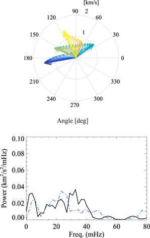
Figure 6. Same as Figure 5 but for Swirl 2.
Download figure:
Standard image High-resolution imageThe analysis of Swirls 3, 4, and 5 shows that, at least in some cases, there are two magnetic structures rotating around one another. This is for instance somewhat clear in Swirl 1, showing the temporal evolution of the photospheric polarization signals. However, a detailed study where the signals in the photosphere spatially resolve this rotation is needed.
3.2. Interaction of Swirls with Acoustic Oscillations
The high-β chromosphere oscillates with a natural period of 3 minutes (e.g., Fleck & Schmitz 1991; Hansteen 1997). In order to investigate the association of acoustic oscillations with swirls, we analyze time series constructed from the average intensity across the FOV in the various channels, using the continuous wavelet transform (CWT; Torrence & Compo 1998) with a Morlet mother wavelet. A time series covers the evolution of the chromospheric plasma before, during, and after the swirl. Different wavelengths across a single spectral line, and between lines, probe physical conditions at different atmospheric heights. Therefore, we use cross correlations between CWTs at different wavelengths to assess physical couplings of plasma in the swirls at different heights (Grinsted et al. 2004). We define the cross-wavelet transform (XWT) of two time series f(t) and g(t) as

where * indicates the complex conjugate. The XWT reveals time intervals and period ranges where the two time series show a common high power (significance) and hence a strong correlation. Significance in the XWTs of two time series is shown using vectors that indicate at each time and period the strength and direction (phase relation) of the correlation. The lag of time series f with respect to time series g is thus represented by the direction (angle). If f is in-phase with g (0°), the correlation vector points to the right. If f is in antiphase with g (180°), the correlation vector points to the left. For a 90° phase lag of f with respect to g, the correlation vector points down. Similarly, for a −90° phase lag (a 90° lead) of f with respect to g, the correlation vector points up.
Swirl 1: we create time series from the Swirl 1 FOV in the various channels for the time interval from 08:21 to 09:05 UT. This covers a time span of 20 minutes before the appearance of the swirl and 7 minutes after the swirl is no longer clearly visible. Their CWTs and XWTs are shown in Figure 7. CWT wavelets corresponding to the various time series are shown in Figure 7. It shows that wave power is enhanced during the swirl. The power of the acoustic oscillations is significant (90%) for a period of 150 s (∼7 mHz frequency) in both Ca ii and Hα. In the absence of swirls, the acoustic oscillations in the chromosphere remain at a constant period of about 180 s. In the presence of the swirl, the power in the oscillation increases, especially in Hα, and the period shortens. The drop in oscillation power immediately before and after the swirl is indicative of a fast change in periodicity. We can conclude that the presence of Swirl 1 modulates the natural chromospheric oscillation frequency.

Figure 7. Magnitudes of the CWT and XWT for time series constructed over the FOV of Swirl 1, representing chromospheric oscillations before, during, and after the swirl. Row 1: CWT plot in the Ca ii line core and ±0.11 Å wings showing power concentrated at the location of the swirl. Row 2: CWT plot for the Hα line core and ±0.26 Å wings. The cone of influence that covers the edge effect is overplotted as solid black lines. Significance levels (%) for the CWT plots are shown by color bars at the bottom of the CWT plots. Row 3: XWT plots showing correlation between Ca ii wings at ±0.11 Å (first panel), between −0.11 Å and the Ca ii line core Å (second panel), and between the Ca ii line core and +0.11 Å (third panel). Row 4: XWT plots showing correlation between Hα Å wings at ±0.26 Å (first panel), −0.26 Å and the Hα line core (second panel), and the Hα line core and +0.26 Å. The color bars below the plots show correlation power. The red box in the first panel indicates the time interval when the swirl appears.
Download figure:
Standard image High-resolution imageThe XWTs are shown in Figure 7. In Ca ii we note that in terms of phase lag the blue wing leads the line core by 90°, which in turn leads the red wing by 90°. In this scenario, we expect the XWT of the two Ca ii wing time series to be in antiphase. However, we find a 90° phase relation instead. We note that the XWT for those two time series has low power, so its phase relation is in doubt. Also, though the period is moderated, the XWT phase relations themselves are not changed by the appearance of the swirl. In Hα, the phase relations are more complex. We look at the phase relations for the first and second halves of the swirl time interval. For the first time half, the blue wing leads the line core by 90°, which in turn slightly leads the red wing. In the second half, roles are reversed. The blue wing has a tendency to lag the line core, which in turn slightly lags behind the red wing.
Swirl 2: we create time series from the Swirl 2 FOV in the various channels, for the time interval from 08:12 to 09:05 UT. The swirl starts at 08:23 UT and lasts for 16 minutes. Their CWTs and XWTs are shown in Figure 8. In Ca ii we detect an oscillation with a period between 230 and 300 s, with a tendency of the period to increase from 230 s at the beginning to 300 s near the end of the swirl. Before and after the swirl, the oscillation period is about 300 s. The presence of this swirl seems to reduce the oscillation period, but it is less pronounced than in Swirl 1. In Hα we only clearly detect an oscillation during the time of the swirl in the line core. Compared with Ca ii, the maximum oscillating power is located between 150 and 180 s. We are possibly detecting different acoustic modes that are locally dominant at different heights in the atmosphere.

Figure 8. CWT and XWT plots for time series constructed over the FOV of Swirl 2, representing chromospheric oscillations before, during, and after the swirl. Column 1, rows 1–3: CWT plot at +0.11 Å, Ca ii 8542 Å line core, and −0.11 Å. Column 2, rows 1–3: CWT plot at −0.26 Å, Hα 6563 Å (row 2), and +0.26 Å. The COI that covers the edge effect is overplotted in solid black lines. Significance levels (%) for the CWT plots are shown by color bars at the bottom of the CWT plots. Column 1, rows 4–5: XWT plots showing a correlation between Ca ii 8542 Å (row 4) and wings at ±0.11 Å. Column 2: XWT plots showing a correlation between Hα wavelengths 6563 Å and wings at ±0.26 Å. The color bars below the plots show the correlation power. The red box in the first panel shows the location of the swirl.
Download figure:
Standard image High-resolution imageThe XWT for Ca ii shows in terms of phase correlation that the line core leads the red wing, which in turn leads the blue wing. However, note that the swirl signature in the line position −0.11 Å is not clear. Because in Hα the signal is only clear in the line core, the XWT for this line is inconclusive.
We have also examined the wavelet and cross-wavelet transforms for line position time series for Swirls 3, 4, and 5. The results are less clear with reduced significance. Swirls 3 and 4 have oscillation periods around 200 s and no clear moderation in oscillation period during the swirl. Swirl 5, like Swirl 2, shows an oscillation with a periodicity between 200 and 300 s that has a trend toward larger period during the swirl. In Hα this periodicity, as well as some evidence for a 120 s period, is seen. In Ca ii, we find a similar correlation phase in the XWTs as for Swirl 1 for all three swirls. In Hα, Swirls 4 and 5 do not show anything significant, but Swirl 5 shows a phase pattern similar to Swirl 1.
Furthermore, considering Ca ii, the time series for the acoustic oscillation for all swirls (where significant) show the same periodicity in the core and in the wings. If the change in intensity in the various line positions is due to Doppler velocity, then a sinusoidal profile of the acoustic velocity would lead to a doubling of the oscillation frequency in the line-core time series (per cycle in the velocity time profile, a blue or redshifted antinode only occurs once, but a node occurs twice). We do not see this. This suggests that the velocity time profile has an asymmetric shape. The line core of the Ca ii line is formed at about 1500 km or less. This is above the height where three-minute acoustic waves are expected to start to form shocks and show asymmetric velocity profiles (Carlsson & Stein 1995, 1997). Also, the XWT phase relations between the core and wings in Ca ii can be reproduced in a simple model that uses synthetic time series evaluated at the core and wings of a Gaussian spectral absorption line that is Doppler-shifted by an asymmetric velocity time profile. For some of the swirls, the oscillation correlation phases in Hα are influenced by the swirl itself. Detailed forward-modeling of the interaction of a swirl and acoustic oscillations would be required to elucidate this further.
The results from wavelet analysis suggest that we most likely see a modification of the acoustic oscillations due to the magnetic structure propagating from the photosphere to the chromosphere. In the swirl there may be temperature increments, which are most likely related to the intensity enhancements observed in the fragments of the swirl in the Hα line core. A temperature increase leads to an increase in sound speed and hence a decrease in period at the same wavelength. A change in periods from 300 to 150 s represents a temperature increase by a factor of 2.
3.3. Rotation and Expansion of Swirls
The motion that evolves in the swirl from the photosphere to the chromosphere is observed to rotate and expand. We investigate the dynamics within a swirl by introducing a polar coordinate system (r, φ) centered on the swirl. We visually track the swirl center in time in the Ca ii red wing and fit a polynomial to the center x and y coordinates to obtain a smooth center track. As before, we show our analysis for Swirl 1 and Swirl 2. Figures 9 and 10 show the Ca ii line core and ±0.11 Å. The signature of the swirl is obvious in Ca ii but much less clear in the Hα red wing and has been omitted. The images are true-type where the R, G, and B channels correspond to the red wing, line core, and blue wing, respectively. There is a clear periodicity in intensity over time across the whole swirls that is linked to previously mentioned chromospheric acoustic oscillations. The phase relations of the oscillations seen in various line positions, which were revealed in Section 3.2, are apparent here as well. Note that, to enhance the detailed dynamics within the swirl from the overlying acoustic oscillation, we rescale at each time the intensity with the average intensity across the whole FOV of the swirl. We cannot eliminate the acoustic signal completely, but differences in phase at different locations of the swirl become apparent in the time–distance plots.
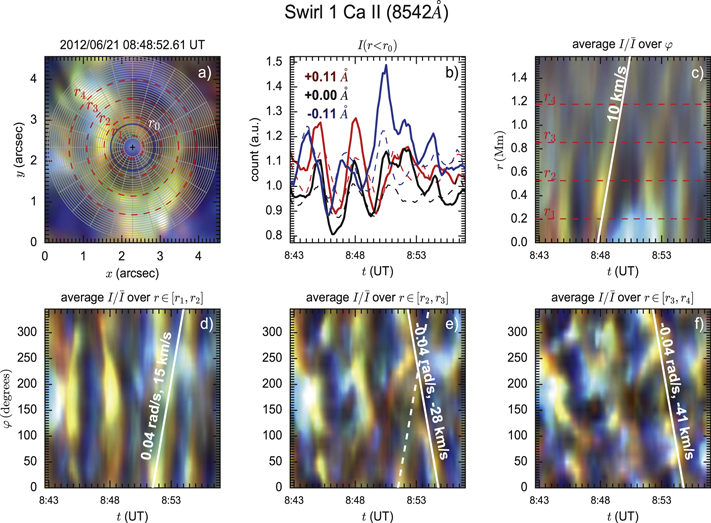
Figure 9. Polar time–distance plots for the ±0.11 Å from Ca ii 8542.0 Å of Swirl 1. Images are true-type where the R, G, and B channels correspond to the blue wing, core, and red wing line positions. (a) FOV centered on the swirl. A polar coordinate system (r, φ) centered on the swirl is superimposed. (b) Integrated intensity within the radius r0 as a function of time for the three line positions. The dashed lines represent the intensity as a function of time integrated across the whole FOV. (c) Angularly integrated intensity as a function of radius r and time. A radial speed of 10 km s−1 has been superimposed. (d)–(f) Radially integrated intensity in the intervals [r1, r2], [r2, r3], and [r3, r4], respectively. A counterclockwise and clockwise rotation of 0.04 rad s−1 has been superimposed as a solid and dashed line, respectively.
Download figure:
Standard image High-resolution image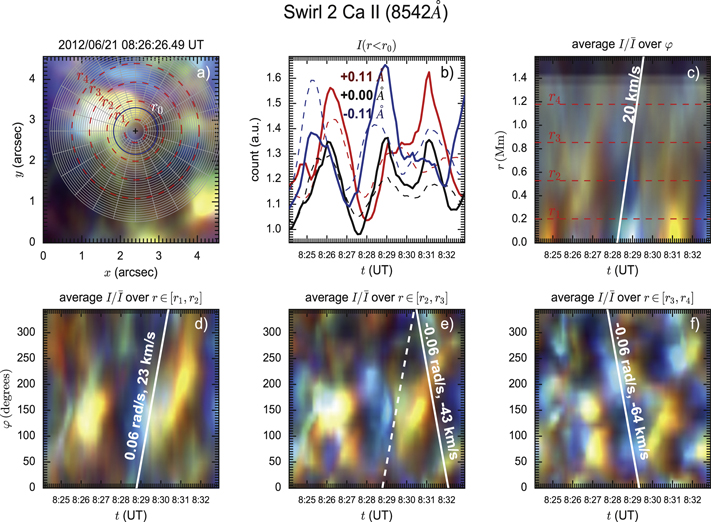
Figure 10. Polar time–distance plots for the ±0.11 Å and Ca ii 8542 Å of Swirl 2. Caption same as for Figure 9.
Download figure:
Standard image High-resolution imageSwirl 1: Figure 9 shows polar plots corresponding to Swirl 1 in Ca ii. In the integrated intensity plot calculated within radius r0, we see continuous intensity enhancements related to the swirl. These have a period of ≈200 s, as observed in Section 3.2. These patterns of low and high intensities are also seen in the radial time–distance plots showing that there is a continuous average radial speed of 10 km s−1 associated with the swirl. Furthermore, the angular time–distance plots reveal clear signatures of rotation, which become more apparent at larger radius. For Swirl 1, there is some suggestion it is rotating in a counterclockwise direction at a rate of about 0.04 rad s−1 (160 s periodicity), while the outer region rotates clockwise at the same rate.
Swirl 2: Figure 10 shows polar plots corresponding to Swirl 2 in Ca ii 8542 Å. As in Swirl 1, Swirl 2 forms a similar radial time–distance plot that shows a continuous radial signal propagation at an average speed of 20 km s−1. A counterclockwise and clockwise rotation of 0.06 rad s−1 (105 s periodicity) has been superimposed as a solid and a dashed line.
In addition, Swirl 4 and Swirl 5 show radial and angular patterns, whereas Swirl 3 does not show any clear radial or angular patterns. Swirl 4 shows a counterclockwise rotation at the rate of 0.045 rad s−1 near the center, slowing down to 0.03 rad s−1 near the arms. Swirl 5 shows a counterclockwise rotation of 0.03 rad s−1 in the outer regions. The swirl rotation is not dissimilar to the periodicity of the motion of the underlying photospheric MCs.
4. Discussion
We have analyzed an SST data set between 08:07:24 and 09:05:46 UT on 2012 June 21, composed of imaging spectroscopic data in Hα and Ca ii 8542 Å wavelengths as well as in spectropolarimetric data in Fe 6302 Å. We have detected 13 candidate chromospheric swirls. Of those, we have analyzed the five most promising swirls in more detail, and details of two of those are presented. The observations reveal cospatial multiwavelength evidence of chromospheric swirls observed in imaging spectroscopic data in Hα and Ca ii wavelengths, as well as in the photosphere. Thus, we present a physical picture that involves connecting the dynamics of the swirl across the photosphere and the chromosphere. We shall first summarize the main findings from the observations.
Previously, chromospheric swirls have mostly been reported in Ca ii only. Here we report for the first time observations of swirls not only in Ca ii but also in Hα. Swirls have a fragmented appearance in Hα. Swirls appear in chromospheric images as a circular pattern in intensity of about 2 Mm in size, which contain rotating arcs or arms of increased intensity that extend from the center to the edge. We have focused on identifying swirls that appear circular at least at one time instant. Out of the 13 detected candidate swirls, we found five clear examples where the circular pattern can be observed almost throughout their lifetime, for 9–10 minutes on average. Doppler imagery shows that at the center of the swirl there is an upflow with a speed in the range of 2–6 km s−1, similar to what has been reported earlier (e.g., Wedemeyer-Böhm et al. 2012). The outer part of the swirl shows alternating Doppler signals, with a single direction in a circular shell around the center at some time or with opposite directions on opposing sides. These variations are in large part due to the acoustic chromospheric oscillations that are superimposed on any flows seen in the swirl. It is therefore difficult to find evidence of up (or down) flows in the line of sight in the outer part of the swirl.
By examining the swirls in polar coordinates, we deduce the radial and angular (rotational) velocities from projected displacements of the swirl arms in intensity. Swirls tend to expand radially with a projected speed of approximately 10–20 km s−1, which is comparable to if not larger than the local sound speed. Furthermore, the swirl rotates clockwise near the center and counterclockwise toward the edge with a period of 100 s for Swirl 1 and 150 s for Swirl 2. The rotation near the center is less certain because of the smaller speeds there compared to at the edge.
Superimposed on the swirl are periodic variations in intensity with a typical period of 180 s, consistent with three-minute chromospheric acoustic oscillations. We have discovered that during the occurrence of the swirl the acoustic oscillation is temporarily altered, that is, reduced in period to 150 s and with an increased or decreased local intensity. A change in period may be due to a change in the acoustic cavity dimensions, additional magnetic effects, or an increase in temperature. If we assume that this change is solely due to temperature, based on the period change, we estimate an upper limit of the temperature increase of 44%. For Swirl 1, we see that during the time interval of reduced periodicity, the swirl appears brighter in the Hα red wing. For Swirl 2, the acoustic power decreases, and there is no clear intensity increase seen in Hα, but we still see intensity enhancements in the arms of the swirls. The phase analysis between the signals in the wings and line core for the chromospheric channels shows in Ca ii that the blue wing precedes the line core, which in turn precedes the red wing. This pattern is always present and is not altered by the appearance of the swirl. The absence of half-period oscillations in the line core compared with the wings suggests that the velocity time series is not sinusoidal but rather asymmetric. This seems consistent with the physical picture of three-minute acoustic waves forming shocks below the formation height of Ca ii around 1500 km. The phase relations in Hα are more complex, which is perturbed during the appearance of some of the swirls. We have not found evidence for the generation of acoustic oscillations by a swirl. Forward-modeling of line formation in simulations of swirls in the presence of acoustic waves would be needed to establish the exact physical picture.
We have chosen to classify chromospheric swirls according to whether they appear above a single or multiple magnetic concentrations located in the intergranular lanes in the photosphere. MCs are visible in Fe i Stokes-V at least 5 minutes before the appearance of a swirl and exhibit various motions and morphological changes before and during the appearance of a swirl. First, in some cases, the morphology of MCs tends to change from appearing stretched and fractured to compact and circular. Some 2–3 minutes after the concentration becomes compact, a swirl appears with a central brightening in Ca ii. For such a time delay and a typical formation height of Ca ii of 1500 km or less, this suggests a travel speed of around 10 km s−1. This is comparable with the typical value of the Alfvén speed in the chromosphere. Second, MCs exhibit periods of rotational or transversal motions about a central point, with speeds of the order of a few km s−1. This motion seems consistent with a magnetic element moving in a larger photospheric vortex flow field. In fact, such motions are fairly common (see Stangalini et al. 2017) with up to 10% of identified MCs in the current data set exhibiting low-frequency rotational motions. However, in the majority of cases, no overlying chromospheric swirl is seen. But for the swirl-associated MCs, these motions have periodicities of around 100–200 s, comparable to the rate of rotation of the chromospheric swirl. Third, MCs also contain various high-frequency motions, with a predominant periodicity of around 30 s. We expect that any low-frequency transversal oscillatory signal propagating upward along the magnetic field can be identified as an Alfvénic kink wave (e.g., Terradas et al. 2010) in the presence of transverse structuring. We do not actually see any difference in the appearance between swirls associated with one or multiple MCs. That may suggest that a swirl is basically associated with a single magnetic concentration. Any neighboring MCs have only a secondary role.
The physical picture that emerges from the observations is that a swirl is a flux tube that extends above a photospheric MC that is located in a downdraft region in an intergranular lane, that is, a local magnetic flux tube moving in a larger (vortex) flow field (confirming Shelyag et al. 2011). The rotational motion of the MC around the flow center seems to be responsible for the signature seen in the chromosphere. As the position of the flux tube moves, we see in the chromosphere the signature of the flux tube position as it moves around a common center. With height, the magnetic field expands radially, and the flux tube has an increased radius for rotation. For an average Alfvén speed of 10–20 km s−1, the typical travel time from the photosphere to the formation height of the chromospheric lines is 150–300 s. Therefore, for photospheric rotation with a longer period, a swirl will not be apparent as the flux tube will practically be at the same location for all heights. For periods comparable to or shorter than the travel time, at chromospheric heights, the flux tube will be lagging behind the photospheric motion. The swirl arm is thus a snapshot of the flux tube seen in line-of-sight integrated projection. As we do not see any clear evidence of an oscillatory pattern in the swirl dynamics at the photosphere, we cannot decide whether a swirl is a gradual motion in response to the photospheric motion or an actual propagating wave. But, the shorter the periodicity compared with the travel time, the more likely it is to be a wave. The most likely wave candidate is a Alfvénic kink wave that has a significant circular polarization as opposed to linear polarization. It is unlikely to be a azimuthally symmetric torsional Alfvén wave as it is unclear how such a wave would break azimuthal symmetry and manifest swirl arms in intensity. It is important to add the caveat that there is not necessarily a one-to-one correspondence between the motion of signature intensity and actual velocities, as revealed by numerical forward-modeling studies (Verma et al. 2013; Louis et al. 2015).
Critically, our study finds that the existence of magnetic concentration, vorticity, and rotational motions in the photosphere is a necessary but not sufficient condition for the existence of a swirl. The timings in photospheric morphology indicate that MCs need to be compact as well to trigger the swirl in the chromosphere.
J.S. is funded by STFC grant ST/P000320/1. The Swedish 1 m Solar Telescope is operated on the island of La Palma by the Institute for Solar Physics of Stockholm University in the Spanish Observatorio del Roque de los Muchachos of the Instituto de Astrofisica de Canarias. This work used the DiRAC Data Centric system at Durham University, operated by the Institute for Computational Cosmology on behalf of the STFC DiRAC HPC Facility. DiRAC is part of the National E-Infrastructure. The authors acknowledge observers Prof. Robertus Erdelyi and Dr. Nabil Freiji. J.S. thanks the High Altitude Observatory for support of a visit during the summer of 2018. P.G.J. is grateful to the coauthors at University of Warwick for a delightful visit early in 2018 when the interpretation of the chromospheric data was started. Armagh Observatory and Planetarium is grant-aided by the N. Ireland Department of Communities. J.G.D. acknowledges the DJEI/DES/SFI/HEA Irish Centre for High-End Computing (ICHEC) for the provision of computing facilities and support. J.G.D. also thanks STFC PATT T and S and the Solarnet project, which is supported by the European Commissions FP7 Capacities Programme under grant Agreement No. 312495 for T and S. S.W. is supported by the SolarALMA project, which has received funding from the European Research Council (ERC) under the European Union's Horizon 2020 research and innovation programme (grant agreement No. 682462), and by the Research Council of Norway through its Centres of Excellence scheme, project number 262622. E.S. would like to thank the International Space Science Institute (ISSI) for supporting the workshop on "The Nature and Physics Vortex flows in Solar Plasmas." We acknowledge the referee for valuable insights into the paper.
Appendix: Summary
Here we present a summary of swirls that are observed in the chromospheric Ca ii 8542 Å line core and the wings at ±0.11 Å, the Hα line core, and the red wing at 0.26 Å. All of the swirls occur above MCs in the photosphere. We could classify swirls into two categories: (1) associated with two or more MCs and (2) associated with one MC. These swirls have an average diameter of 2 Mm and a lifetime between 9 and 10 minutes. Of the 13 swirls mentioned in the Figure 11, 11 showed clearly fragmented signals in Hα. Column 2 shows a context image corresponding to the swirls. The crosshairs on the images show the centers of the observed swirls. Column 3 shows P as position in arcseconds. Column 4 shows that lifetime T is the time that is estimated when we see and track by eye the swirl in Ca II. Column 5 contains the diameter D calculated when the swirls show a clear ring-like appearance. Column 6 containts comments on the respective swirls.

Download figure:
Standard image High-resolution image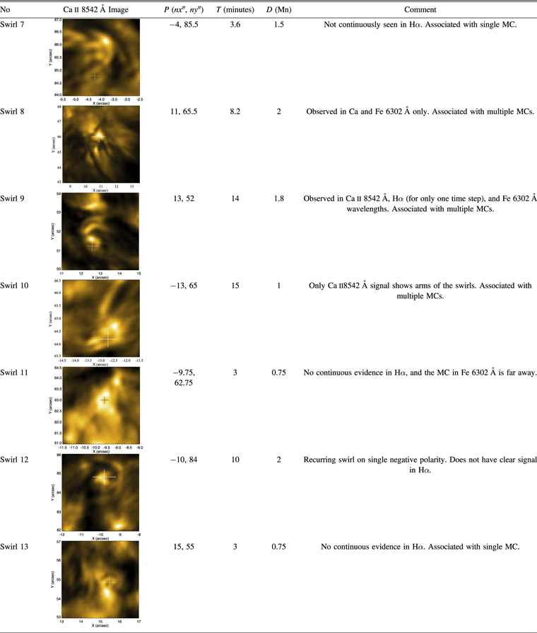
Figure 11. Summary of the properties of swirls observed in the data set. P is position in arcsec. Lifetime T is the time that is estimated when we see and track by eye the swirl in Ca ii. Diameter D is calculated when the swirls show a clear ring-like appearance. Crosshairs on the images show the centers of the observed swirls.
Download figure:
Standard image High-resolution image