


Abstract
The mixing of convective overshoot is quite uncertain in low-mass stars. To study the mixing in the convective core and beyond the convective boundary for low-mass stars, we use the k–ω model, which is proposed by Li. We determine that the distance of the overshooting region is about 0.072 in the 1.3 M⊙ star. There are two parts in the overshooting region, one is the completely mixing region of about
  , and the other is the partial mixing region of about 0.045
 . Next, we study the semiconvection for low-mass stars. We find that the semiconvection near the convective core boundary can be removed when we use the k–ω model. Then, we calibrate the
  for classical overshooting by using the k–ω model. As a result, we find that a suitable value of
  is about 0.008 for the mass range of 1.0–1.8 M⊙ stars.
Export citation and abstract BibTeX RIS
1. Introduction
In the mass range of 1.0–2.0 M⊙ stars, the CNO cycle may produce more energy than the PP chain, so a convection region occurs in the central part of the star. As the star evolves, the mass of the convective core expands gradually. There will be a discontinuity on the hydrogen profile at the border of the convective core. As a result, a semiconvective region develops naturally above the convective core because of the opacity contribution to the radiative temperature gradients according to Paxton et al. (2018, 2019). The mixing in the semiconvective region is very uncertain in stellar models. Langer et al. (1983) proposed a numerical approximation model based on the linear analysis of Kato (1966). Spruit (1992) used the diffusion coefficient to deal with semiconvection based on the double diffusive picture. Different methods may produce different mixing efficiency, leading to great differences in the stellar models.
The mixing of convective overshoot is also uncertain in the mass range of 1.0–2.0 M⊙ stars. Overshooting is a region that extends beyond the convective boundary as determined using the Schwarzschild or the Ledoux criteria, and where mixing is assumed to be efficient enough to completely mix the elements according to Gabriel et al. (2014). The convective overshoot has an important influence on the structure and evolution of the star. It increases the hydrogen fuel of the convection region, leading to the time of the star during the main sequence to be prolonged. Finally, a larger helium core is left at the center of the star. There are several methods to treat the convective overshoot. For example, Herwig et al. (1997) proposed a model that is based on the 2D hydrodynamical simulations from Freytag et al. (1996).
Its diffusion coefficient is expressed as:
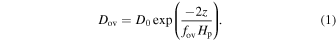
Among them, D0 is the diffusion coefficient of the convective core boundary, z is the geometric distance to the boundary of the convection core,  is the local pressure scale height, and
  is a free parameter for governing the convective overshoot width. The distance of the convective overshoot region, however, has an important influence on the evolution of the stars. Claret & Torres (2017) found that the magnitude of convective overshoot varies with the stellar mass and evolution stage. Xiong & Kimura (1981) and Xiong (1986) proposed a nonlocal model to treat the convective overshoot region. Recently, Li (2012, 2017) proposed the k–ω model. It is based on fluid dynamics and more suitable to treat turbulent convection of the stars. The k–ω model can describe not only the convection zone but also the convective overshoot zone. It has been successfully applied to the solar and stellar models in Li (2017).
To study the mixing in the convective core and beyond the convective boundary for low-mass stars, we use the k–ω model that is appropriate in both the convective core and the overshooting region. We briefly describe the k–ω model in Section 2 and introduce physical input in Section 3. Our main results are shown in Section 4. Our summary and discussion are provided in Section 5.
2. The k–ω Model
The k–ω model was proposed by Li (2012, 2017). It is based on the fluid dynamics. Moreover, it can calculate the convection region and convective overshoot region of the stars. It has been used for the solar models and sdB models (Li 2017; Li et al. 2018). The k–ω model has eight free parameters. It mainly uses two equations to describe the turbulent convection of the stars. The two equations are related to κ and ω, where κ is the turbulent kinetic energy and ω is the turbulence frequency.
The equation for the turbulent kinetic energy κ is:
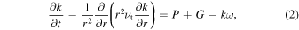
where P is the shear production rate of the turbulent kinetic energy, and G is the buoyancy production rate of the turbulent kinetic energy.
The equation for the turbulence frequency ω is:
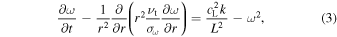
L is a macro-length of turbulence. According to common choices (Pope 2000) the model parameters are  ,
,  , and
, and  .
.
The macro-length of turbulence by Li (2017) is:

where  is the radius of the convective core, and
  is an adjustable parameter.
In Equations (3) and (4) the turbulent diffusivity  is:
is:

The diffusion equation of element abundance can be written as:

where  is the generation rate of element i,
  is the mass fraction, and
  is the diffusion coefficient of any mixing process.
 is given by Li (2017):
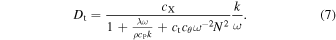
 and
and  are two model parameters, whose values are given by turbulence models according to Hossain & Rodi (1982).
  is an adjustable parameter. ρ is the density. P is the total pressure.
  is the specific heat at constant pressure.
The equation of the buoyancy frequency N:

where g is the gravity acceleration. T is the temperature. ▽ is the actual temperature gradient, and  is the adiabatic temperature gradient.
The equation of the thermodynamic coefficient β is:

λ is the radiation diffusivity:
σ is the Stefan–Boltzmann constant. κ is the Rosseland mean opacity. Through the Equations (2), (3), and (7) we can figure out κ, ω, and  . For more details, please see Li (2012, 2017).
3. Input Physics
We calculate our stellar models by Mesa (Modules of Experiments in Stellar Astrophysics), which was developed by Paxton et al. (2011, 2013, 2015, 2018). The version of Mesa we have used is 11554. The Schwarzschild criterion and convective premixing are adopted to determine the convection zone.
The initial masses are 1.3 M⊙, 1.4 M⊙, 1.6 M⊙, 1.8 M⊙, and 2.0 M⊙. The initial metallicity is Z = 0.02. We calculate the evolution of the stars from zero age to the end of the main sequence. The nuclear burning network includes the PP chain and the CNO cycle for the hydrogen-burning process. We use the OPAL opacities calculated using the GN93 composition (Grevesse & Noels 1993). The boundary condition for the atmosphere is the Eddington gray atmosphere. For comparison, we deal with convection and convective overshoot in two different ways. One is the standard stellar model (ST model), which uses the standard mixing-length theory. We use the mixing-length parameter α = 1.8 according to solar calibrations. The boundary of the convection zone is determined by the Schwarzschild criterion. The method of Herwig et al. (1997) is used in the overshooting stellar model (OV model) for the convective overshoot region. We use the free parameters  for 1.3 M⊙ star,
  for 1.4 M⊙ star,
  for 1.6 M⊙ star, and
  for 1.8 M⊙ star.
Another way to deal with convection and convection overshoot is the k–ω model (KO model). We incorporate it into Mesa through "run star extras. f" package. In the "run star extras. f" package, we get the diffusion coefficients by solving Equations (2), (3), and (7). The parameters of the k–ω model are shown in Table 1. These parameters  ,
,  , α, and
  in Table 1 are calibrated according to the solar model in Li (2012, 2017).
  ,
,  , and
, and  are common choices according to the Pope (2000).
  and
and  are two model parameters, whose values are given by turbulence models according to Hossain & Rodi (1982).
Table 1. Parameters of the k–ω Model
 . . |
 . . |
 . . |
ct. | ch. | cx. | α. |
 . . |
|---|---|---|---|---|---|---|---|
| 0.09 | 1.5 | 0.5 | 0.1 | 2.344 | 0.01 | 0.7 | 0.06 |
Download table as: ASCIITypeset image
4. The Convection of Low-mass Stars During the Main Sequence
The evolutionary tracks of the 1.3 M⊙ star are shown in Figure 1, which displays the stellar models with the different overshooting mixing schemes. It can be seen that the two lines are almost identical, which are for the stellar models with the overshooting mixing schemes of the k–ω model and Herwig (2000). Compared with the ST model that is computed without considering the overshooting effects, the two overshooting models show higher luminosities and have the main-sequence turning points with lower effective temperatures.
Figure 1. Evolutionary tracks of the considered 1.3 M⊙ star modes. One line is for the stellar model with the Schwarzschild criterion and without overshooting. The other two lines are for stellar models with the overshooting mixing schemes of the k–ω model and Herwig (2000).
Download figure:
Standard image High-resolution image4.1. The Convective Overshooting in the 1.3 M⊙ Star
In the mass range of 1.2–2.0 M⊙, a small convective core emerges during the main sequence. With the evolution of the stars, the temperature at the stellar center gradually increases. It leads to a growing contribution of the CNO cycle reactions. As the CNO cycle contribution increases, the mass in the convective core expands gradually.
The profiles of turbulent kinetic energy and turbulence frequency are shown in Figure 2 during the main sequence. We indicate the Schwarzschild boundary by the vertical dotted line, where  . It can be seen that the turbulent kinetic energy is about 105 in the convective core. It is interesting to note that the turbulent kinetic energy falls quickly near the center, where the local pressure scale height is infinite at the stellar center. The turbulent kinetic energy is inversely proportional to the local pressure scale height according to Li et al. (2019). On the other hand, an overshooting region forms beyond the surface of the convective core, because a significant amount of turbulent kinetic energy is transported outside the convection core by the turbulent diffusion effect. In Figure 2, the turbulent kinetic energy and turbulence frequency both decrease in the overshooting region. Figure 3 shows the distribution of Dt as a function of the fractional mass. We find that Dt is about 1012 in the convection core. Such a big Dt illustrates that there is a complete mixing in the convective core. In the overshooting region, however, Dt suddenly drops to about 105 and then continues to decrease exponentially. This means that there is a partial mixing in the overshooting region.
Figure 2. Distributions of the turbulent kinetic energy and the turbulence frequency compute with the k–ω model of the  star. The vertical dotted line is the Schwarzschild boundary of the convective core.
Download figure:
Standard image High-resolution image
Figure 3. Dt as a function of the fractional mass in the k–ω model of the  star. The vertical dotted line is the Schwarzschild boundary of the convective core.
Download figure:
Standard image High-resolution imageThe detailed structure of the overshooting region is shown in Figure 4 for a model of 1.3 M⊙ star during the main sequence. It can be seen from the distribution of the turbulent diffusion coefficient in the upper panel of Figure 4 that the distance of the overshooting region is about 0.072 in the 1.3 M⊙ star. It can be seen from the hydrogen profile in the lower panel of Figure 4 that there are two parts in the overshooting region by the k–ω model, one is a completely mixing region of about
  , and the other is a partial mixing region of about 0.045
 . Our result is similar to the overshooting mixing scheme proposed by Herwig (2000), which is widely adopted. For comparison, the distribution of turbulent diffusion coefficient for stellar model with the overshooting mixing scheme of Herwig (2000; OV model) is shown in Figure 5. The vertical dotted line is the Schwarzschild boundary. We can see that the distance of overshooting region is about
  for the OV model in the 1.3 M⊙ star. It can be seen from the hydrogen profile of the OV model in Figure 5 that there are also two parts in the overshooting region, one is a completely mixing region of about
  , and the other is a partial mixing region of about 0.031
 . It is interesting to note that although the distances of complete mixing regions of the KO model and OV model are the same, the partial mixing region of the KO model is wider than that of the OV model. It can be seen from Figure 6 that Dt of the OV model presents exponential decay with a bigger constant slope. However, Dt of the KO model suddenly drops to about 105 and then continues to decrease exponentially. As a result, there is a wider partial mixing region for the KO mode. It is worth noting in Figure 7 that in the overshooting region, the KO scheme results in a smoother transition than the OV scheme does. A smooth transition in the chemical profile is important for the astroseismological requirements.

Figure 4. Distributions of the radiative temperature gradient, adiabatic temperature gradient, hydrogen abundance profile, and Dt compute with the k–ω model of the  star. The value of the initial hydrogen is x = 0.7. The vertical dotted line is the Schwarzschild boundary of the convective core.
Download figure:
Standard image High-resolution image
Figure 5. Distributions of the radiative temperature gradient, adiabatic temperature gradient, hydrogen abundance profile, and Dt compute with the OV model of the  star. The value of the initial hydrogen is x = 0.7. Z = 0.02 and α = 1.8 for the OV model. The vertical dotted line is the convective core boundary, which is determined by the Schwarzschild criterion and convective premixing.
Download figure:
Standard image High-resolution image
Figure 6. Dt compute with the classical overshooting and the k–ω model for the 1.3 M⊙ star, Z = 0.02, and α = 1.8 for the OV model, the parameters of the k–ω model in Table 1. The vertical dotted line is the Schwarzschild boundary of the convective core.
Download figure:
Standard image High-resolution image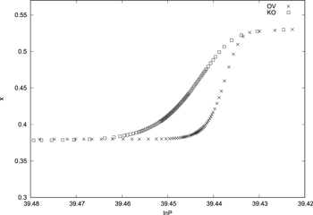
Figure 7. Hydrogen abundance profiles compute with the classical overshooting and the k–ω model for the 1.3 M⊙ star, Z = 0.02, and α = 1.8 for OV model, the parameters of the k–ω model in Table 1.
Download figure:
Standard image High-resolution image4.2. Semiconvection in the Mass Range of 1.2–2.0 M⊙ Stars
When a convective core appears near the chemical gradient region, mixing in this region may become quite uncertain. It depends on which mixing scheme is used (complete mixing,partial mixing or not mixing) and which stability criterion is adopted (Ledoux criterion or Schwarzschild criterion). In Figure 8 (left panel), standard treatments of convection in MESA 5 (including convective premixing in the convective core). This approach introduces a problematic result that a small burr appears on the radiative temperature gradient and a small step shape appears on the hydrogen profile in the semiconvection region. Furthermore, in Figure 9 (left panel), some unexpected points appear on the convective core mass profile for 1.3 M⊙, 1.4 M⊙, 1.6 M⊙, and 1.8 M⊙ stars. The primary reason of this phenomenon is that the semiconvection region is mixed into the convective core, leading to the convective core mass suddenly increasing. Fortunately, this phenomenon does not appear in the 2.0 M⊙ star.
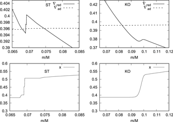
Figure 8. Radiative temperature gradient, adiabatic temperature gradient, and hydrogen abundance distributions computed with the Schwarzschild criterion (left panel) and the k–ω model (right panel) in models of the  star. Z = 0.02 and α = 1.8 for the ST model, the parameters of the k–ω model in Table 1.
Download figure:
Standard image High-resolution image
Figure 9. Convective core mass as a function of the central hydrogen abundance computed with the Schwarzschild criterion (left panel) and the k–ω model (right panel). Z = 0.02 and α = 1.8 for ST model, the parameters of the k–ω model in Table 1.
Download figure:
Standard image High-resolution imageThe semiconvection, however, does not appear in the k–ω model. We can see in Figure 8 (right panel) that the radiative temperature gradient and the chemical abundance are continuous. In the k–ω model, the Schwarzschild boundary has been clearly defined, because the radiative temperature gradient is always larger than the adiabatic temperature gradient in the whole convection zone, and the jump of the chemical abundance does not appear. when we adopt the mixing scheme with the k–ω model in Figure 9 (right panel), the convective core mass profiles remains smooth for stars of all masses, and the unexpected points seen in the left panel of Figure 8 do not appear. The reason of this phenomenon is that the k–ω model contains the convective overshoot region, so the mixing scheme with the k–ω model is equivalent to adding a convective overshoot region in the stellar model, and the overshoot mixing can remove the discontinuous points and the semiconvection region. Our result is similar to that of Meng & Zhang (2014). They found that the overshoot mixing can remove semiconvection in the mass range of 1.2–2.0 M⊙ stars. A similar method was adopted by Noels (2013) to deal with the mixing of the semiconvection region. Xiong & Kimura (1981) and Xiong (1986) found that the semiconvection is due to the local convection theory and they solved this problem by using the nonlocal turbulent convection theory. We have a similar result that the nonlocal effect of turbulent convection, overshoot mixing, can remove semiconvection in the mass range of 1.2–2.0 M⊙ stars.
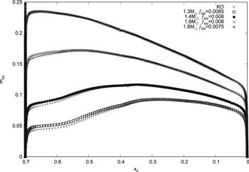
4.3. Calibrating the  for Classical Overshooting with the k–ω Model

The value of  is a free parameter for the classical overshoot. It is determined usually by comparisons of stellar models with the observations. In order to get a suitable value of
  , we compare the classical overshoot model and the k–ω model, and Figure 10 shows the fractional convective core mass as a function of central hydrogen abundance computed with the classical overshoot model and the k–ω model. We get the best-fit state for the two lines to calibrate the
  by the k–ω model. We find that a suitable value of
  is about 0.008 for the mass range 1.0–1.8 M⊙ stars. Our result is different from that of Claret & Torres (2017). They found a mass dependence that
  rises sharply from zero in the range 1.2–1.8 M⊙ stars. In recent years, some investigations have shown that the overshooting depends on the stellar mass. Schroder et al. (1997) found that in the mass range of 2–7.2 M⊙, the overshooting distance increases with the stellar mass from about
  to
to  by studying nine double-lined eclipsing binary (DLEB) stars. Ribas et al. (2000) found that in the stellar mass range of 2–12 M⊙, the amount of overshooting increases with the stellar mass from a study of six DLEB stars. Stancliffe et al. (2015) found no clear trend in the overshooting by using 11 DLEB pairs. Valle et al. (2016) found that in the mass range of 1.1–1.6 M⊙, there are many theoretical uncertainties in the stellar models, for example, helium content, radius, Teff, metallicity, mixing-length, mass, and element diffusion. They concluded that the method for calibrating the overshoot is unreliable.
Figure 10. Fractional convective core mass as a function of central hydrogen abundance computed with the OV model and the KO model, Z = 0.02 and α = 1.8 for the OV model, and the parameters of the k–ω model in Table 1.
Download figure:
Standard image High-resolution image
Overall, we do not find that overshooting depends on the stellar mass, which is similar to Constantino & Baraffe (2018) and Stancliffe et al. (2015). Our result is that a suitable value of  is about 0.008 for the mass range of 1.0–1.8 M⊙ stars.
5. Conclusions and Discussion
Mixing is quite uncertain in the convective overshooting region and the semiconvection region, which has an important impact on the stellar evolution. To study the structure of the convective overshooting region in low-mass stars, we calculate the overshooting region for a 1.3 M⊙ star using the k–ω model. We determine that the distance of the overshooting region is about  . There are two parts in the overshooting region, one is the completely mixing region of about
  , and the other is the partial mixing region of about 0.045
 . For comparison, we also calculate the stellar model with the overshooting mixing scheme of Herwig (2000). We find that the partial mixing region of the KO model is wider than that of the OV model.
In the mass range of 1.0–1.8 M⊙ stars, a semiconvection region occurs near the boundary of the convective core. We use the k–ω model for the semiconvection region, then the semiconvection is removed. The k–ω model includes not only a convective unstable zone but also an overshooting region. Our result is similar to that of Meng & Zhang (2014). They found that the overshoot mixing can remove semiconvection in the mass range of 1.2–2.0 M⊙ stars. We also find that in the standard stellar model, some unexpected points appear on the convective core mass profile for 1.3 M⊙, 1.4 M⊙, 1.6 M⊙, and 1.8 M⊙ stars. However, the convective core mass profiles remain smooth for stars of all masses, and the unexpected points do not appear in the k–ω model.
The  is a free parameter of the OV model. Its value is determined usually by comparisons of stellar models of the observations. We calibrate the value of the
  by using the k–ω model. Our result is that a suitable value of
  is about 0.008 for the mass range 1.0–1.8 M⊙ stars.
In summary, we can get the distance of the overshooting region using the k–ω model. The semiconvection does not occur when we use the k–ω model. In the mass range of 1.0–1.8 M⊙ stars, the value of the  is about 0.008.
This work is funded by the NSFC of China (grant Nos. 11333006 and 11521303).