


Abstract
The ribbon of enhanced energetic neutral atom flux, discovered by the Interstellar Boundary Explorer (IBEX) in 2009, has redefined our understanding of the heliosphere's interaction with the local interstellar medium (LISM). Yet, its origin continues to be a topic of scientific debate. The ribbon is circular and traces the region where the putative LISM magnetic field (BLISM) is perpendicular to the radial direction from the Sun. Using nine years of IBEX-Hi observations, we investigate the ribbon circularity and location as functions of time and energy. We provide updated locations of the ribbon center at five energy passbands (centered at 0.7, 1.1, 1.7, 2.7, and 4.3 keV) in ecliptic coordinates [longitude, latitude]: [217 41 ± 095, 4436 ± 093], [21972 ± 095, 4150 ± 087], [22051 ± 119, 3996 ± 100], [21808 ± 166, 3844 ± 124], and [21468 ± 148, 3413 ± 119] respectively. The weighted mean center location over all energies and all years is [21833 ± 068, 4038 ± 088] and its radius is 7481 ± 065. As viewed by IBEX at 1 au, we find that (1) the ribbon is stable over time, with distinct centers at each energy; (2) ribbon centers exhibit small temporal variations, likely caused by the solar wind (SW) speed and density variations; and (3) ribbon location in the sky appears to be driven by (i) the inherent alignment of the ribbon centers along the plane connecting the presumed BLISM and the heliospheric upwind direction, and (ii) the variable SW structure along the heliographic meridian, further emphasizing that the ribbon source is outside the heliosphere.
Export citation and abstract BibTeX RIS

Original content from this work may be used under the terms of the Creative Commons Attribution 3.0 licence. Any further distribution of this work must maintain attribution to the author(s) and the title of the work, journal citation and DOI.
1. Introduction
The heliosphere is a bubble-like structure cocooned in the local interstellar medium (LISM). It is created by the continuous outflow of magnetized solar wind (SW) from the Sun. The supersonic SW slows down abruptly forming the termination shock (TS). Upstream of the TS, The boundary between the LISM and the slowed-down SW is the heliopause (HP), and is formed where the total LISM pressure balances the SW pressure. As the interstellar neutrals drift through the heliosphere, some of them become ionized through charge exchange or photoionization and are then picked up by the SW flow, becoming pick-up ions (PUIs). In the heliosheath region between the TS and the HP, cold interstellar neutral atoms interact with the shocked (slowed down and heated at the TS) outflowing SW ions, and with the PUIs via charge exchange, creating energetic neutral atoms (ENAs). Some of these ENAs travel back to 1 au carrying inherent signatures of their progenitor ion populations (e.g., Gruntman et al. 2001; Heerikhuisen et al. 2008; Prested et al. 2008). These ENAs, which are called the globally distributed fluxes (GDFs; McComas et al. 2009b) provide a unique remote sensing capability that enables us to understand the global properties and interactions of different energetic ion populations in the heliosheath and beyond.
The Interstellar Boundary Explorer (IBEX) mission (McComas et al. 2009a) continues to image the heliospheric-LISM interactions covering almost a full solar cycle of observations. Among the numerous discoveries of the dominant physical processes at the heliospheric boundaries (McComas et al. 2017), the most notable is the discovery of a ribbon of enhanced ENA emissions across the sky. The ribbon appears in IBEX-Hi and IBEX-Lo at energies ∼0.2–6 keV and is most pronounced between ∼1 and 3 keV. It is almost circular (wrapping nearly ∼300° around the sky), narrow (∼20°–40° in width depending on the energy), and its center lies in the vicinity of the pristine magnetic field direction of the LISM (Frisch et al. 2012), whose field lines are draped around the heliosphere. The ribbon intensity is, on average, a factor of 2–3 times higher than that of the more diffuse, GDF ENA flux and varies as a function of energy (Funsten et al. 2009; Fuselier et al. 2009; McComas et al. 2009b, 2014; Schwadron et al. 2009).
Numerous mechanisms have been suggested for the source of the ENA ribbon (see the summary in McComas et al. 2014). With numerous lines of evidence from IBEX, McComas et al. (2017) argued that "the nominal explanation of the Ribbon going forward" is a secondary ENA mechanism (e.g., McComas et al. 2009b, 2014, 2017; Heerikhuisen et al. 2010; Möbius et al. 2013; Schwadron & McComas 2013; Giacalone & Jokipii 2015; Zirnstein et al. 2015, 2016a, 2017; Swaczyna et al. 2016). In this mechanism, as the interstellar neutrals penetrate into the heliosphere, they charge exchange with the supersonic SW ions. These newly neutralized SW atoms (known as "primary" ENAs) travel into the outer heliosheath (beyond the heliopause), unaffected by magnetic and electric fields. Once in the outer heliosheath, they undergo two sequential charge exchange events: an ionization event followed by another neutralization event, creating "secondary" ENAs. The direction of motion of these atoms and the location of the charge exchange are critical for these secondary ENAs to be observed at 1 au (e.g., Heerikhuisen et al. 2010; Zirnstein et al. 2015). Secondary ENAs with pitch angles close to 90° in the radial direction (i.e., perpendicular to the direction of the interstellar magnetic field inferred from simulations, B · R ∼ 0), or those spatially retained near B · R ∼ 0 (Schwadron & McComas 2013), traveling radially can be observed at 1 au (e.g., Zirnstein et al. 2016b), and thus appear as a circular ribbon of enhanced emissions in the sky. In this work, we define the B–V plane as the vector between the interstellar magnetic field (B) location inferred from simulations using the ribbon location and constrained by Voyager data (Heerikhuisen et al. 2014; Zirnstein et al. 2016b), and the LISM inflow vector determined by McComas et al. (2015).
Almost 10 years into the mission, IBEX have enabled us to peek into the variability and time lags affecting ribbon ENA emissions. Schwadron et al. (2018) separated the ribbon from the ENA GDF using a transparency masking method and found that the ribbon ENAs vary at timescales that are distinct from the surrounding GDF observed over the rest of the sky, suggesting that both signals are generated from two different parent populations. Using a ribbon-centered frame of reference, Funsten et al. (2013) studied the spatial properties of the IBEX ribbon using the first three years of IBEX observations. They determined an averaged ribbon center at ecliptic [λRC, βRC] =[2192 ± 1.3, 399 ± 23] and an angular radius of φC =745 ± 20. The ribbon center was found to shift systematically with energy. A difference of ∼10° was found between ribbon center locations at low and high ENA energies. Ribbon simulations with latitude-independent SW boundary conditions by Zirnstein et al. (2016a) observed a systematic shift as a function of energy, but did not appear to explain the largest shift at the highest ENA energies.
The intensity of ENA emission around the ribbon varies with time. McComas et al. (2012) found that temporal variations of ENAs are correlated with the supersonic SW latitudinal structure around solar minimum. These authors found that the slow SW (∼400 km s−1) primarily affects low energy (∼1.1 keV) ribbon ENAs observed at low latitudes, intermediate-speed SW affects ENAs (∼1.7 keV) observed at mid-latitudes, and high-speed SW (∼760 km s−1) is most reflected in high energy (∼2.7 keV) ENAs observed primarily at high latitudes.
Funsten et al. (2015) exploited these intensity variations and found that the ribbon exhibits a flux symmetry between the ribbon center and the upstream heliospheric direction (B–V plane) as a function of energy: at 1.7 keV, the axis of symmetry nearly matches the B–V plane; at 2.7 and 4.3 keV, the symmetry axis is shifted by about +30° off the B–V plane; and at 0.7 and 1 keV, the symmetry axis is about −30° from the B–V plane. They suggested that the B–V plane appears to play an organizing role in the symmetry of the ribbon fluxes. Zirnstein et al. (2016a) simulated the influence of ENA energy and SW speed, independent of time and latitude, on the global spatial and geometric properties of the ribbon. Those authors found a strong dependence of the simulated ribbon energy spectrum and spatial symmetry on SW speed and ENA energy, but only a slight dependence on ribbon geometry. These results agreed qualitatively with Funsten et al. (2015) and further suggested that flux ribbon ordering is possibly a mixture of the latitudinal asymmetry of the SW and the interaction of the SW with the LISM.
Furthermore, Zirnstein et al. (2016a) found that under uniform SW conditions (i.e., fixed SW speed with no slow/fast structure), the ribbon centers are shifted almost parallel to the B–V plane as a function of ENA energy, with the center of the highest energy being the closest to the center of the pristine LISM direction, suggesting a critical role of the asymmetric LISM field draping in creating such behavior. Swaczyna et al. (2016) used an analytical model of the ribbon (see also Möbius et al. 2013) to study the ribbon position in the sky, without accounting for the LISM field draping around the heliosphere. They found that the systematic variability in the geometric center of the ribbon by about 10° as a function of energy is a consequence of the helio-latitudinal structure of the SW reflected in the secondary ENAs. The authors suggested that this further emphasizes the likelihood of the secondary ENA emission mechanism as the source of the ribbon. Furthermore, they attributed the magnitude of the center shift in the highest IBEX energy channel to another process of ENA generation that is yet to be recognized.
The location of the IBEX ENA ribbon is thus critical to understanding its sources, structure, and creation mechanisms, the LISM field direction, as well as quantifying the role that the SW structure plays in shaping the ribbon. In this work, we use 9 yr of IBEX-Hi observations between 2009 January and 2017 December to study the evolution of the ENA ribbon center location as functions of energy and time. Both quantities convolve variability of the SW structure as a function of the solar cycle activity. Data and observations are discussed in Section 2; the analysis methodology is discussed in Section 3; results are discussed in Section 4; and the implications of the results on our current understanding of the IBEX ribbon position in the sky are discussed in Section 5.
2. Data and Observations
Throughout this analysis, we use IBEX-Hi, 6° × 6° resolution, annually combined, ENA sky maps during 9 yr between 2009 January and 2017 December at five different energy passbands, centered at 0.7, 1.1, 1.7, 2.7, and 4.3 keV. Data have been acquired from the IBEX Science Operations Center, which periodically validates and provides data to the official IBEX data release website, publicly accessible at http://ibex.swri.edu/researchers/publicdata.shtml (see also McComas et al. 2017; Schwadron et al. 2018). The data set combines the Ram and the anti-Ram sky maps for improved counting statistics and incorporates two important ENA corrections: (1) Survival probability, which accounts for the survivability of ENAs from 100 to 1 au, and (2) Compton–Getting correction, which accounts for the spacecraft motion with respect to the measured ENAs. We correct for these two effects such that we remove effects of losses to ENAs in the supersonic SW and the maps are transformed into the solar inertial frame of reference. Following the ribbon-centered frame analysis illustrated in Funsten et al. (2013), we remap the IBEX sky maps originally in the ecliptic coordinates onto a ribbon-centered spherical coordinate system (azimuth, polar) = (θ, ϕ) centered on ecliptic (2185, 431), (2203, 405), (2196, 398), (2179, 377), and (2142, 324) for energy passbands centered on 0.7, 1.1, 1.7, 2.7, and 4.3 keV respectively. These values were inferred by Funsten et al. (2013) using the first three years of IBEX observations. The azimuth angle θ ranges from 0° to 360° around the ribbon center counterclockwise, with 0° aligned with the heliospheric nose in the upwind direction, and ϕ being the angular distance from the ribbon center to any point in the sky (i.e., half-cone angle and hereafter, the ribbon radius). Assuming that the ribbon center is aligned with the LISM magnetic field, the B–V plane is thus defined in this frame to be along the positive horizontal axis (running from left to right), passing through the center of the ribbon and heliospheric nose. Figure 1 shows the ∼1.1 keV ENA sky map, time-averaged during 2009–2011, in the ribbon-centered frame at ecliptic [2203, 405] as determined in Funsten et al. (2013), along with indications to different directions in the sky.

Figure 1. ENA fluxes of the 2009 sky map at 1.1 keV in the ribbon-rotated frame centered at ecliptic [2203, 405]. Labels indicate locations of the direction of upwind (nose) and downwind (tail) interstellar inflow, Voyagers 1 and 2 (V1 and V2), and the ecliptic north and south poles (NP and SP).
Download figure:
Standard image High-resolution imageFigure 2 shows the ribbon-centered sky maps obtained by IBEX during 2009–2017 (columns) and for five IBEX-Hi energy passbands (rows). Each combined sky map in this figure comprises a statistical combination of an annual RAM and anti-RAM map. Consistent color-coding is shown for each energy passband over all years for comparison purposes.

Figure 2. Annual IBEX-Hi ENA flux maps (rows) for five energy passbands (columns) in the ribbon-centered frame (see Figure 1 for directions in the sky). The reference frames of the ribbon-centered maps at energies 0.7, 1.1, 1.7, 2.7, and 4.3 keV are centered on ecliptic (latitude, longitude) coordinates derived by Funsten et al. (2013; see the text for details). ENA flux data is corrected for the ENA survival probability and for the Compton–Getting effect.
Download figure:
Standard image High-resolution imageThe figure clearly shows the evolution of ENA emission over time at each energy step. The first three years stand out as the brightest ENA emissions at all energies. Fluxes then gradually dim at different rates through 2016. The most prevalent dimming is clear at the highest two energy passbands, 2.7 and 4.3 keV. In 2017, ENA emissions at energies above 1.7 keV start to increase, reflecting the response of the heliosphere-LISM system to a preceding increase in the SW ram pressure, due to solar activity, as predicted and substantiated in McComas et al. (2017, 2018b) respectively (see also Schwadron et al. 2018; Zirnstein et al. 2018).
3. Methodology of the Analyses
To further improve the counting statistics, we statistically combine the annual maps in four different time intervals from 2009 to 2017. The first combined map set includes the first three IBEX sky maps (acquired 2009 January through 2011 December), the second combined map set includes the next two sky maps (2012 January–2013 December), the third combined map set includes two subsequent maps (2014 January–2015 December), and the fourth combined map set includes the most recent two sky maps (2016 January–2017 December). The four different combined sets thus represent four intervals of temporal changes over nine years. The combination helps reduce the flux uncertainties and increase exposure time in each pixel used to construct the full sky map. On average, combined annual maps in each set also had comparable fluxes at each of the energy passbands, so the large variations in the ENA fluxes observed over time are maintained (McComas et al. 2014, Schwadron et al. 2018). For instance, maps at 4.3 keV in Figure 2 show bright enhancements of similar order during 2009–2011, dimmer maps during 2012–2013 and 2014–2015, and then brighten up during 2016–2017.
Figure 3(a) shows the combined map sets. The orientation of the map sets is similar to those in Figure 2. We derive the geometric properties of the ribbon by fitting a circle to the peak fluxes along the ribbon. To determine the peak fluxes along the ribbon, we used a similar approach to the fitting procedure used in Funsten et al. (2013) (also in Zirnstein et al. 2016a), with the improvement that we account for the statistical ENA flux uncertainties in every pixel. For each 6° azimuthal sector, we fit ENA fluxes with a Gaussian function of the form

where A is the baseline flux (i.e., ENA GDF level), B is the height of the Gaussian (i.e., ENA peak flux), ϕ is the polar distance, ϕc is the location of the Gaussian center (i.e., ENA peak flux location at a certain azimuth), and σG is the Gaussian width. We note that the function does not allow determination of the skewness that might be present in the ribbon. Yellow dots on each map set of Figure 3(a) indicate the fitted peak of ENA flux along the ribbon for each individual 6°, azimuthal sector, derived using the four-parameter Gaussian fit to the ribbon flux along the polar direction. The solid black line indicates the circularity fit using the fitted peaks.
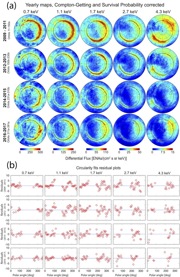
Figure 3. (a) ENA fluxes of the combined map sets [2009, 2010, 2011], [2012–2013], [2014–2015], and [2016–2017]. This combination enhances the statistics to reveal systematic temporal variation of ENA emission over the nine years of ENA measurements. Azimuthal slices through the ribbon are used to fit the ribbon peak (within the 30°–120° polar angle from the map center) to a Gaussian distribution. Yellow dots indicate the location of the maximum of the Gaussian fit within the corresponding 6° azimuthal sector. Black lines indicate the uncertainty-weighted circular fits, derived using the yellow points. (b) Residuals of the circularity fits shown in (a).
Download figure:
Standard image High-resolution imageData selection has been a nontrivial aspect of this study. Given that we currently do not have a full understanding of the ribbon shape, sources, and variability, there is virtually no way to fully and precisely examine its evolution. However, a robust way forward that we found is to use a universal criterion that fits the data for all years examined (2009 through 2017). Funsten et al. (2013) utilized the first three years of data, where ENAs were most pronounced in the sky. Since then, ENAs have dimmed in different regions and at different rates. The criteria that we used appeared to provide the largest number of points in fitting the data for all years. After numerous trials using different functions to describe the ribbon, we decided to use region selections that are based on the brightest ENA ribbon emissions during the first three years, and are similar for the most part to Funsten et al.'s (2013) work. The region of magnetospheric viewing in the sky is easily singled out based on the spacecraft location and viewing, the magnetospheric extent in the sky, and the "bad times" that appear in the raw orbital data as high noise, prior to running the maps. Public released maps are already validated and contain the good-times only, which we use in this work. Moreover, the region with the magnetospheric contamination has already been identified in Funsten et al. (2013), which is what we use here.
We fit the Gaussian function to ENA ribbon fluxes in every 6° azimuthal sector in a 42° range along the polar direction (ϕ). Some azimuthal sections should be excluded from the analysis. At 0.7, 1.1, and 1.7 keV, we exclude sections between 123° and 195°, as this region contains the heliotail lobes structure (McComas et al. 2013) and the noisy region of the magnetospheric obstruction to IBEX's field of view in the sky, both are features with ENA sources independent of the ribbon. At higher energies, the ribbon exhibits a bimodal symmetry (Funsten et al. 2015) and almost vanishes near low latitudes. We thus exclude these sections where ENA fluxes from the ribbon are dimmest and at the GDF level. These are the azimuthal sections between 309°–9° and 93°–195° for 2.7 keV channel, and between 303°–9° and 93°–195° for 4.3 keV channel. Similar to Funsten et al. (2013), we also ignore azimuthal sections that produced uncertainties greater than 2° in determining the location of peak flux from the Gaussian fit (ϕc) for 0.7–2.7 keV, and ignore sections with uncertainties greater than 3° for the 4.29 keV passband. These uncertainty thresholds follow from the fact that the ribbon is slightly wider at higher energies, and present a tight constraint on having a viable fit. Setting such criteria further constrains the peak location determination at each azimuth. That being said, for >90% of the cases, the errors are well within these criteria and very few points got excluded due to this particular condition.
Finally, we also ignore sections where  , thus excluding regions of low ribbon fluxes compared to the underlying GDF. We note here that a significant effort was performed to improve the ribbon fitting, including (i) averaging more than 6° azimuthal sectors to improve the statistics, (ii) using non-Gaussian and Gaussian-like distributions to fit the ribbon shape, (iii) using a discrete selection criteria and a fitting function for the ribbon at each energy passband. However, these attempts to improve the fit had no noticeable effect on the overall results. The current analysis appears to best describe the ribbon geometry with as few free parameters as possible.
Figures 4 and 5 shows all fits for the 1.1 and 4.3 keV ENA sky maps for 2009–2011. Fits marked with a green dot on the bottom left of each panel indicate that these azimuthal sectors are included in the analysis, and those with a red dot are excluded from the analysis because they failed to pass the selection criteria. Similar results are obtained for ENAs at the remaining energies.
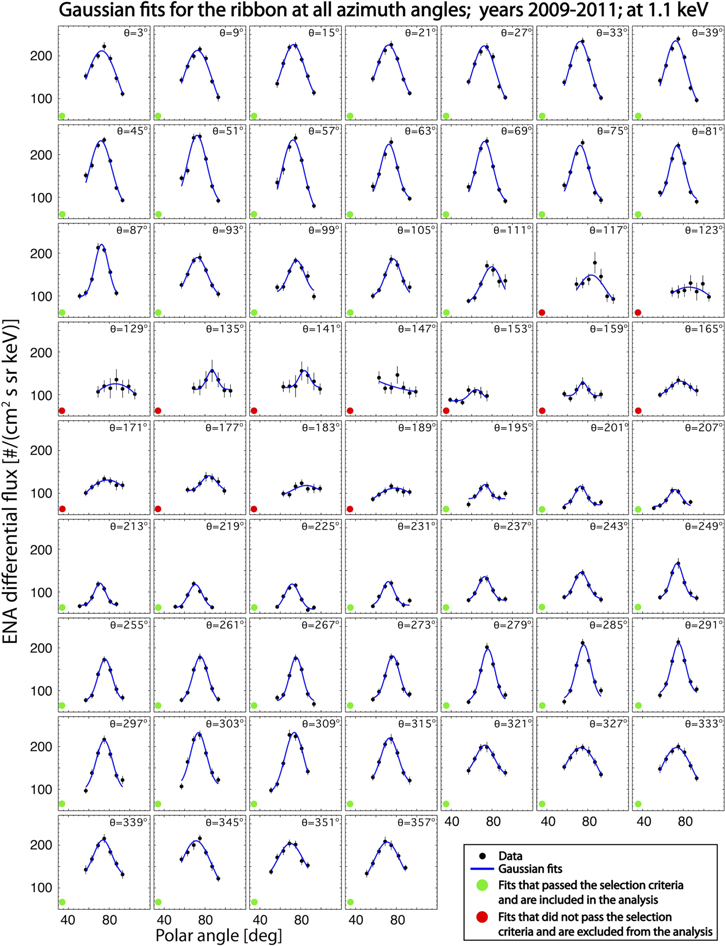
Figure 4. Gaussian fits for ribbon fluxes at all azimuth sectors for the combined years [2009, 2010, 2011] at 1.1 keV. The angle θ corresponds to the azimuthal angle from the ribbon center-heliospheric nose vector.
Download figure:
Standard image High-resolution image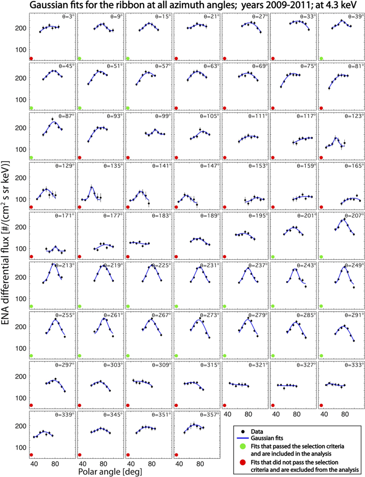
Figure 5. Same format as Figure 4 but for the combined years [2009, 2010, 2011] at 4.3 keV.
Download figure:
Standard image High-resolution imageAfter determining the peak flux fits for each 6° azimuth sector, we fit a circle to the locations of ϕc associated with all sectors using the Levenberg–Marquardt least-squares minimization (Markwardt 2009). Following Zirnstein et al. (2016a), the uncertainties in determining ϕc were used as weights for the circularity fits. Circularity fits to each map result in a circle center and its mean radius. The circle center is weighted by the uncertainties in the maximum flux locations, and the mean circle radius is the averaged mean distance of each maximum flux location from the derived circle center. The uncertainty in the ribbon center and radius (later referred to as δ) is determined by computing the standard deviations of the maximum flux locations (ϕc) from the mean radius.
Figure 3(b) shows the residuals of the circularity fits for all maps in Figure 3(a). Residuals are randomly distributed around the zero line for all energies except for the 1.1 keV, where a periodic-like trend is visible. The existence of this periodic trend in the residuals also exists in the more general elliptical fit to the data (not shown). This trend is an indication of nonlinearity (e.g., curvature) effects that are not captured well by the circularity fit. The circularity fit is driven by the peaks inferred from the Gaussian fits of the individual ENA profiles along azimuth sectors. Furthermore, Funsten et al. (2015) showed that the ribbon exhibits a sagittal symmetry that is also a function of energy. Taken together, we suggest that the combined effect of peak variations along the fitted circle and the symmetry in these peak fluxes are reflected in the residual trends. This can further be clarified once the ribbon is measured at a better spatial resolution (e.g., with Interstellar Mapping and Acceleration Probe (IMAP); McComas et al. 2018a), in which a more precise function can then be used to fit the ribbon and accounts for any skewness and/or flatness of the fitted ENA profile (e.g., shape parameter).
Table 1 lists the derived ribbon centers and radii in ecliptic coordinates for IBEX-Hi energy channels. The table shows the time-weighted mean values of the ribbon centers at each energy. Here, the mean is weighted by the inverse variance of the derived quantities. For a given set of ribbon centers at four time periods,  , where xi could represent longitude, latitude, or radius of the ribbon, the weighted mean is calculated as

where the weights are defined as  .
.
Table 1. Circularity Fitted Parameters Along with the Weighted Mean Values
| Time Range | Fitting Parameter | IBEX-Hi Energy Passbands (keV) | ||||
|---|---|---|---|---|---|---|
| 0.7 | 1.1 | 1.7 | 2.7 | 4.3 | ||
| 2009–2011 | λ[°] | 216.90 | 220.65 | 221.35 | 218.73 | 213.97 |
| β[°] | 44.63 | 41.42 | 40.00 | 38.68 | 34.61 | |
| ϕ[°] | 75.79 | 73.33 | 72.86 | 74.15 | 77.59 | |
| δ[°] | 1.25 | 1.92 | 1.48 | 2.17 | 1.53 | |
| N | 34 | 47 | 42 | 33 | 23 | |
| 2012–2013 | λ[°] | 218.31 | 220.68 | 220.76 | 219.34 | 216.84 |
| β[°] | 44.32 | 42.07 | 40.36 | 38.35 | 33.59 | |
| ϕ[°] | 75.10 | 73.38 | 73.41 | 75.43 | 79.98 | |
| δ[°] | 2.04 | 2.36 | 2.17 | 2.08 | 2.06 | |
| N | 19 | 48 | 44 | 32 | 24 | |
| 2014–2015 | λ[°] | 217.23 | 219.32 | 221.02 | 218.82 | 212.57 |
| β[°] | 44.89 | 41.70 | 38.96 | 37.53 | 32.53 | |
| ϕ[°] | 75.34 | 73.19 | 74.21 | 75.86 | 81.54 | |
| δ[°] | 2.68 | 1.91 | 2.46 | 3.09 | 5.18 | |
| N | 26 | 40 | 38 | 23 | 16 | |
| 2016–2017 | λ[°] | 217.89 | 219.21 | 218.36 | 214.12 | 213.06 |
| β[°] | 43.49 | 41.29 | 40.20 | 38.95 | 33.91 | |
| ϕ[°] | 73.30 | 73.08 | 73.66 | 75.81 | 81.21 | |
| δ[°] | 1.94 | 1.26 | 2.03 | 2.79 | 3.58 | |
| N | 24 | 40 | 33 | 20 | 15 | |
| weighted mean | λ[°] | 217.41 ± 0.95 | 219.72 ± 0.95 | 220.51 ± 1.19 | 218.08 ± 1.66 | 214.68 ± 1.48 |
| β[°] | 44.36 ± 0.93 | 41.50 ± 0.87 | 39.96 ± 1.00 | 38.44 ± 1.24 | 34.13 ± 1.19 | |
| ϕ[°] | 75.10 ± 1.06 | 73.19 ± 0.86 | 73.36 ± 1.01 | 75.17 ± 1.28 | 78.86 ± 1.48 | |
Note. λ: ecliptic longitude; β: ecliptic latitude; ϕ: angular radius; δ: uncertainty in the center and radius; N: number of points used in the fit.
Download table as: ASCIITypeset image
The uncertainty of the mean values (σm) is determined as the root of the squared sum of the propagated error (σp) and the statistical uncertainties (σs) of the four values, given by

where the propagated errors are

and the statistical uncertainties are determined as (e.g., see Zirnstein et al. 2016b)
Following these equations, the weighted mean center location over all energies and all years (20 data points) is [21833 ± 068, 4038 ± 088] and its radius is 7481 ± 065.
4. Circularity Analysis Results
Figure 6 shows the derived ribbon centers in ecliptic coordinates as a function of energy (color-coded) and time (symbols). Centers for each energy passband are clustered together and appear to maintain distinct locations for all years, with overlapping uncertainties. The ribbon is remarkably stable over time at each energy, with the largest temporal changes occurring at the lowest (0.7 keV) and the highest (4.3 keV) energy passbands. Another noticeable trend is the southward migration of the ribbon center with increasing energy (Funsten et al. 2013). As shown, the higher the energy, the lower the latitude location of the ribbon center. This is an anticipated effect of the ribbon's location being closer to the northern than the southern heliospheric pole, as will be discussed later on.

Figure 6. (a) Derived ribbon centers over five energy passbands (color-coded) and for the four different time periods considered in this study (symbols).
Download figure:
Standard image High-resolution imageFigure 7 shows the variation of the derived ribbon centers as functions of ecliptic longitude (panels (a) and (b)) and latitude (panels (c) and (d)). For the first three time periods, Figure 7(a) shows that the ribbon centers indicate opposite behavior pivoting around the 1.7 keV value; the centers' longitudes increase at low energies (0.7, 1.1 keV) and decrease at high energies (2.7, 4.3 keV). Figure 7(b) shows that no significant trend appears as a function of time. Instead, there exist small variations (within the uncertainties) that may be due to the variable SW structure, which would affect the location of the ribbon center in both longitude and latitude.
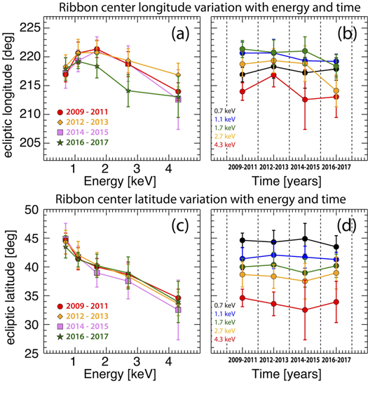
Figure 7. (a) Variation of the derived ribbon centers over five energy passbands (color-coded) and for the four different time periods (symbols) as functions of longitude (panel (a) and (b)) and latitude (panels (c) and (d)).
Download figure:
Standard image High-resolution imageIn terms of latitudinal variations, the ribbon center evolves in a monotonic pattern: the higher the energy, the lower the ribbon center's latitudinal location, as shown in Figure 7(c). As will be shown later, a kendall tau analysis of this trend shows that it is statistically significant. However, there is no statistically significant change of the ribbon center latitudes as a function of time (Figure 7(d)).
Figure 8 shows the variation of the derived ribbon circular radii as functions of energy and time. The ribbon is smallest and most stable with the smallest temporal fluctuations occurring at 1.1 and 1.7 keV, and the largest fluctuations occurring at 4.3 keV. At this energy, the ribbon gets wider as time progresses over the first three time periods, and stabilizes during the last time period.
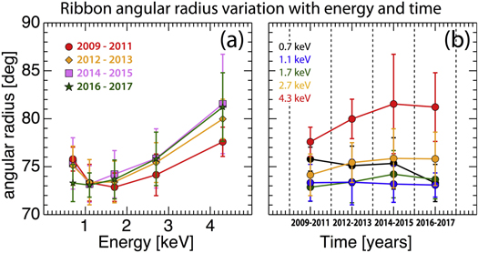
Figure 8. (a) Variation of the derived ribbon angular radius as functions of (a) energy and (b) time.
Download figure:
Standard image High-resolution imageTo assess the statistical associations strength and direction of the relations shown in Figures 7 and 8, we treat all data points for each plot as ordinal discrete variables. We then rank each plot using the Kendall's Tau (τ) coefficient, which is a nonparametric measure of concordance (Agresti 2002). Table 2 shows the results. In this table, τ < 0 indicates an inverse correlation, τ > 0 indicates a positive correlation, and the p-value determines τ's significance at 0.05 level of significance. Bold values correspond to a significant correlation. This analysis shows that the ribbon center latitudinal motion as a function of energy is statistically significant (Figure 7(c)). In Figure 8(a), the location of the data point at the lowest energy step appears to be the driver behind the significance of the linear trend obtained in the Kendall tau analysis. We note that it is within the uncertainty range of the other data points at the same energy.
Table 2. Kendall's Tau Correlation of the Ribbon Center and Radius as Functions of Time and Energy for all Relations Shown in Figures 7 and 8
| Figure | Correlated Quantities | Varying Parameter (Time or Energy) | Kendall's Tau | Significancea | |
|---|---|---|---|---|---|
| Figure 7(a) | Energy | Ribbon center longitude | Years 2009–2011 | −0.2 | 0.62 |
| Years 2012–2013 | −0.2 | 0.62 | |||
| Years 2014–2015 | −0.2 | 0.62 | |||
| Years 2016–2017 | −0.6 | 0.14 | |||
| Figure 7(b) | Time | Ribbon center longitude | 0.7 keV | 0.33 | 0.49 |
| 1.1 keV | −0.66 | 0.17 | |||
| 1.7 keV | −0.66 | 0.17 | |||
| 2.7 keV | −0.33 | 0.49 | |||
| 4.3 keV | −0.33 | 0.49 | |||
| Figure 7(c) | Energy | Ribbon center latitude | Years 2009–2011 | −1.0 | 0.014 |
| Years 2012–2013 | −1.0 | 0.014 | |||
| Years 2014–2015 | −1.0 | 0.014 | |||
| Years 2016–2017 | −1.0 | 0.014 | |||
| Figure 7(d) | Time | Ribbon center latitude | 0.7 keV | −0.33 | 0.49 |
| 1.1 keV | −0.33 | 0.49 | |||
| 1.7 keV | 0.0 | 1.0 | |||
| 2.7 keV | 0.0 | 1.0 | |||
| 4.3 keV | −0.33 | 0.49 | |||
| Figure 8(a) | Energy | Ribbon angular radius | Years 2009–2011 | 0.2 | 0.62 |
| Years 2012–2013 | 0.6 | 0.14 | |||
| Years 2014–2015 | 0.6 | 0.14 | |||
| Years 2016–2017 | 0.8 | 0.05 | |||
| Figure 8(b) | Time | Ribbon angular radius | 0.7 keV | −0.6 | 0.17 |
| 1.1 keV | −0.6 | 0.17 | |||
| 1.7 keV | 0.6 | 0.17 | |||
| 2.7 keV | 0.6 | 0.17 | |||
| 4.3 keV | 0.6 | 0.17 | |||
Note.
aSignificance values ≤0.05 are considered significant.Download table as: ASCIITypeset image
5. Discussion and Conclusions
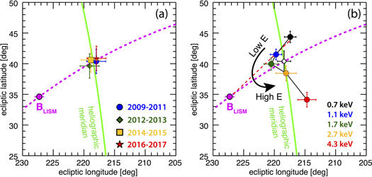
We study the evolution of the circular ribbon radius and center in time and energy. Analysis included more years than previously examined and improved statistics (Funsten et al. 2013). Results indicate that the ribbon remains very circular with distinct centers associated with each energy passband. For each energy, center locations exhibit some temporal variation but they remain clustered together and separate from the other energies with no particular significant trend in time, as illustrated in the Kendall tau analysis. We suggest that these variations may be due to the variable SW structure, which would ultimately affect the ENA flux distributions along the ribbon in both longitude and latitude, resulting in circularity-fitting variations. Figure 9(a) shows the averaged ribbon centers for each time period over all energies. The magenta dashed line traces the B–V plane, where we define the interstellar magnetic field (B) from Zirnstein et al. (2016b), and the LISM inflow vector (V) from McComas et al. (2015). The energy-averaged ribbon center is extremely close to the B–V plane over all years and fluctuates slightly within the derived uncertainties, further indicating that the ribbon, on average, is a very stable object in the sky, regardless of longer-term changes in the SW structure. Table 3 lists the angular distances of the energy-averaged ribbon center for the four time periods covering all years.
Figure 9. (a) Derived ribbon centers over the IBEX-Hi energy range during four different time periods (symbols). (b) Ribbon weighted center locations for each energy passband. The magenta curve traces the B–V plane (BLISM from Zirnstein et al. 2016b, and V from McComas et al. 2015), the green line traces the heliographic meridian, which passes through the solar poles. The pristine interstellar magnetic field direction derived by Zirnstein et al. (2016b) is also shown in magenta. The red dashed line is a fit to the ribbon centers below 1.7 keV and the pristine interstellar magnetic field direction (4 data points; see the text for details). The open diamond symbol is the averaged ribbon center location over all energies.
Download figure:
Standard image High-resolution image
Table 3. Angular Distances of the Energy-averaged Ribbon Center During All Studied Periods
| Years | Longitudes of the Energy-averaged Ribbon Center | Latitudes of the Energy-averaged Ribbon Center | Angular Distance from the B–V Plane |
|---|---|---|---|
| 2009–2011 | 217.99 ± 1.55 | 40.38 ± 1.99 | −0.865 ± 1.625 |
| 2012–2013 | 219.07 ± 1.21 | 39.63 ± 2.11 | −0.840 ± 0.702 |
| 2014–2015 | 218.88 ± 1.54 | 40.61 ± 1.98 | −0.280 ± 1.606 |
| 2016–2017 | 217.95 ± 1.33 | 40.88 ± 1.45 | −0.379 ± 1.180 |
Download table as: ASCIITypeset image
In Figure 9(b), we show the ribbon centers at all energy passbands weighted over time, along with the weighted mean over all energies (diamond symbol). Superposed traces are the B–V plane (magenta) and the heliographic meridian (green) that passes through the solar poles of the Sun. The figure shows an interesting trend: the ribbon center at 1.7 keV is the closest to the B–V plane. At energies below 1.7 keV, the ribbon centers are roughly aligned with the B–V plane but slightly deflected toward the heliographic meridian; the lower the energy, the farther the center from the B–V plane. At energies above 1.7 keV, the ribbon centers show a similar trend of moving farther away from the B–V plane along the heliographic meridian; the higher the energy, the farther the center is from the B–V plane.
We interpret these observations with context from two recent modeling papers. First, Zirnstein et al. (2016a) found that under uniform SW conditions (i.e., fixed SW speed with no slow/fast structure), the asymmetric draping of the LISM B field tends to organize the centers approximately along the B–V plane, and deflected slightly northward, with the highest energy being closer to the pristine B field direction, and thus likely coming from the farthest distance away from the heliopause.
Second, Swaczyna et al. (2016) used an analytical model of the ribbon (see also Möbius et al. 2013) with latitudinal-dependent SW, and examined its position in the sky. Their model does not account for the LISM field draping around the heliosphere. However, they found that the ribbon centers align well with the heliographic meridian and that the systematic variability in the ribbon geometric center by about 10° as a function of energy is a consequence of the helio-latitudinal structure of the SW reflected in the secondary ENAs. The authors suggested that this further emphasizes the likelihood of the secondary ENA emission mechanism as the source of the ribbon. Furthermore, they attributed the magnitude of the center shift in the highest IBEX energy channel to another process of ENA generation that is yet to be recognized. However, their model did not produce an alignment of low energy ribbon center along the B–V plane. This symmetry around the B–V plane at low and high energies has also been reported in Funsten et al. (2015), who found that the ribbon sagittal axis of symmetry tends to behave in tune with the B–V plane.
Taken together with the observations shown in Figure 9, we suggest that there are two main factors that determine the position of the ribbon in the sky, as observed form 1 au. First, the low energy ribbon centers are organized along the B–V plane due to the draping of the interstellar magnetic field around the heliopause (Zirnstein et al. 2016a, 2016b). Second is the breaking of this B–V alignment by the variable SW structure, which breaks this organization by naturally changing the locations of the high energy ribbon centers (susceptible to the fast SW input at high latitudes) along the heliographic meridian (Swaczyna et al. 2016).
The migration of the ribbon center southward with increasing energy provides interesting hints about the structure and the geometry of the ribbon and is a combination of different processes. The asymmetry of the heliosphere (e.g., Reisenfeld et al. 2012) and the asymmetry of the SW structure (e.g., Dayeh et al. 2011, Sokół et al. 2013, 2015) result in an asymmetric contribution of the fast SW at northern and southern high latitudes. Since the ribbon's natural position is much closer to the northern heliospheric pole (by ∼39°), a natural disorder of the ENA fluxes is reflected along the ribbon, which inevitably affects its circularity properties. High energy ENAs produced by fast SW at the north pole have easy access to most of the ribbon spatial structure, while the ENAs coming from the southern heliospheric pole will only populate the outer edge of the ribbon (i.e., the farthest portion away from its peak fluxes in the southern hemisphere), thus bringing the whole structure southward. In fact, that is the same reason that at higher energies, the ribbon expands to much higher latitudes. This expansion was also partially illustrated in Figure 9 of Swaczyna et al. (2016). These authors showed that a quantitatively southern portion of the ribbon moves southward more than the northern portion movement, resulting in a ribbon that shifts southward.
Another factor that relates to the SW variations and plays a role in the ribbon position is the size of the heliosphere. The ram pressure of the SW leaving the Sun inflates or deflates the heliosphere as it varies during the years. While this has already been shown to affect the global variations of the ENA fluxes in the sky (e.g., McComas et al. 2014, Schwadron et al. 2018), changes in the size of the heliosphere may alter the magnetic pressure (e.g., Pogorelov et al. 2011) in the region where the secondary ribbon ENAs are thought to be created, which in turn could affect the secondary ENA generation mechanism, believed to be responsible for the ribbon (see also Zirnstein et al. 2018).
Furthermore, Figure 9(b) also shows the direction of the LISM B field as derived from modeling and fitting to the IBEX ribbon, with constraints by Voyager (Zirnstein et al. 2016b). Interestingly, the location of the ribbon center at energies below ∼1.7 keV align very well with the pristine LISM B direction found in the model of Zirnstein et al. (2016b) far from the heliosphere. The dashed red line represents a linear fit of the B-LISM location far from the heliosphere and the averaged ribbon centers at 0.7, 1.1, and 1.7 keV (dashed red). These ENA energies correspond to slow/medium SW energies, whose variability is minimal at high latitudes, and thus they are not affected by the high latitude SW, when compared to the centers at higher ENA energies. In fact, this could also serve as ground truth evidence for the direction of the LISM B field. Although not included in this analysis, but the ribbon centers at even lower energies (e.g., 0.4 keV) may or may not be aligned with the 0.7–1.7 keV and B-LISM locations, because this low energy ENA population might be coming from different sources, such as the inner heliosheath (e.g., Fuselier et al. 2018). In this case, it would be independent from the LISM.
With the anticipated IMAP mission launching within the coming decade (McComas et al. 2018a), we will be able to quantify and resolve the observed temporal variations of the ENA ribbon structure and its position at a finer resolution, greater precision, and over a broader energy range. IMAP will further refine the apparent motion of the ribbon and provide critical additional information on the sources and the mechanisms affecting the ENA ribbon and the interaction of the LISM with the heliosphere.
This work was carried out as part of the IBEX mission, which is part of NASA's Explorer program. M.D., E.Z., and J.H. acknowledge support from NASA grant 80NSSC17K0597. Work at SwRI was partially supported by NASA grant NNX17AB98G.