


Abstract
In a recent paper, Consolini et al. investigated the statistics of geometrical invariants of the coarse-grained gradient tensor of plasma velocity for a case study of space plasma turbulence. They showed how, at spatial scales near the proton inertial length, there is evidence for the occurrence of dissipation structures along the Vieillefosse's tail. Here, we extend the previous analysis to the statistics of the geometrical invariants of the magnetic field coarse-grained gradient tensor, computed using magnetic field measurements by the ESA-Cluster mission in the solar wind region. In detail, we investigate the evolution of the joint probability distribution functions of the magnetic geometrical invariants at different scales in the inertial range of turbulent solar wind. The results show a clear dependence of the joint statistics of geometrical invariants on the distance from the proton inertial length scale in the inertial range, which seems to be compatible with a variation of the dimensionality of the fluctuation field from two dimensions to three dimensions at the smallest scales. Evidence of an increasing role of the ingoing spiral saddle and current-associated dissipation structures is found at the smallest investigated scales, where dissipation can occur.
Export citation and abstract BibTeX RIS
1. Introduction
The investigation of turbulence in space and an astrophysical context has become a central issue to understanding several dynamical processes related to mass transport, plasma heating, and acceleration, as well as magnetic reconnection (Rai Choudhuri 1998; Carbone & Pouquet 2009). Indeed, turbulence is widely ubiquitous in space and astrophysical plasmas. For instance, in the framework of heliospheric plasmas, turbulence has been shown to occur in several different regions: from the solar corona to the solar wind and the interplanetary medium, from the Earth's magnetosheath to the tail central plasma sheet, etc. Moreover, turbulence seems to play a key role in processes such as anomalous diffusion and fast reconnection. Inside the heliosphere, the solar wind and the interplanetary medium are the regions where the studies on turbulence date back to the early era of space missions, offering, indeed, a natural laboratory for the investigation and modeling of space plasma turbulence in collisionless plasmas (Bruno & Carbone 2005) from magnetohydrodynamic (MHD) scales down to kinetic ones.
The nature of spatiotemporal fluctuations in turbulent fluids and magnetofluid media, such as space plasmas, is very complex due to the highly non-Gaussian and strongly long-range correlated features of these fluctuations and the role that structure formation plays in generating such fluctuations. The last statement is particularly true for turbulent space plasmas where the dynamics of the magnetic field and plasma structures has been shown to play a relevant role in determining the evolution of such plasma systems.
The investigation of the spatiotemporal fluctuations in turbulent space plasmas is generally based on the analysis of single-point observations and on the characterization of the scaling and spectral features of the magnetic field and plasma parameters (density, velocity, temperature, etc.; Zhou et al. 2004; Bruno & Carbone 2005). Although these approaches provided great advances in the comprehension of the turbulent nature of space plasmas, unveiling several mechanisms and the role played by the turbulence in plasma heating and acceleration, little is known about the relevant three-dimensional (3D) topologies responsible for such processes.
In recent decades, the launch of a flotilla of satellites flying in a quasi-tetrahedral configuration, such as the ESA-Cluster and NASA-MMS missions, has provided new opportunities to understand the relevant topologies involved in the dynamical processes (e.g., heating and acceleration) taking place in turbulent space plasmas. Indeed, the availability of multi-point measurements of fields and plasma parameters offers the possibility to obtain more detailed information on the spatial features of the observed fluctuations and their evolution with the scale by the analysis of a finite-scale approximated (coarse-grained) version of the geometric invariants of the plasma velocity and magnetic field gradient tensors, Aij = ∂iuj and Xij = ∂ibj.
Recently, Consolini et al. (2015) have attempted the evaluation of the coarse-grained velocity gradient tensor and its geometrical invariants at small scales for a case study of space plasma turbulence using the ESA-Cluster data, following what has been done in the case of fluid turbulence (Chertkov et al. 1999; van der Bos et al. 2002; Celani et al. 2003; Chevillard & Meneveau 2006; Naso & Godeferd 2012). In particular, they have studied the joint statistics  of the velocity gradient geometric invariants, finding a good similarity to what is expected in the case of the low end of the inertial range for fluid turbulence, i.e., evidence for the occurrence of kinetic energy dissipation due to vortex stretching (Consolini et al. 2015). However, a more comprehensive analysis of the relevant topologies in the case of magnetohydrodynamic turbulence would also include the investigation of the magnetic field gradient tensor features. Indeed, the magnetic field has a fundamental role in determining the relevant topologies of the dissipative structures (Hater et al. 2011; Dallas & Alexakis 2013). Furthermore, numerical simulations (Dallas & Alexakis 2013) evidenced how there are differences between the velocity and magnetic structures involved in turbulence dissipation, the latter being essentially two-dimensional (2D) due to the intrinsic anisotropic nature of magnetized media.
In this work, we investigate the features of the magnetic field topologies at different scales in the turbulent inertial range for a set of ESA-Cluster measurements in solar wind. This study is done following the same approach described in Consolini et al. (2015), i.e., by evaluating the statistics P(RX, QX) and P(Qj, −QK) of the geometric invariants of the coarse-grained magnetic field gradient tensor. It may be useful to clarify that the term geometric invariant here is equivalent to SO3-scalar: the geometric invariants of a tensor are all of the non-vanishing independent quantities that may be formed with its components not changing under 3D rotations, as explained above.
2. Magnetic Gradient Tensor and Geometric Invariants: A Short Review
Understanding the mechanisms and the structures involved in the dissipation and generation of intermittency is central to the study of turbulent media, such as fluids and plasmas. For instance, in this framework, the study of the features of the velocity field gradient tensor, Aij = ∂iuj, can provide relevant information on the role of nonlinear self-stretching in generating large fluctuations at small scales, as well as on the energy transfer between larger/smaller eddies (see, e.g., Vieillefosse 1984; Cantwell 1992, 1993). Additional information can be gained by investigating the features of the magnetic field gradient tensor, Xij = ∂ibj, in the case of plasmas. In particular, the analysis of the geometrical invariants of the magnetic field gradient tensor, constructed by the eigenvalues, can give us the opportunity to figure out the structures that are more involved in the dissipation in turbulent plasmas. Indeed, the gradient tensor of a vector field (as is the case for velocity and magnetic field) can provide information about the local structure of the field lines, which can be classified according to the eigenvalues of the gradient tensor. In other words, the eigenvalues determine the different nature of critical points, which reflects on the local pattern of the vector field.
In analogy with the hydrodynamic case (Cantwell 1992) from the definition of the magnetic field gradient tensor, Xij = ∂ibj (X = ∇b), it is possible to introduce a set of geometrical invariant quantities that characterize the local geometrical features of the magnetic field lines. Clearly, differently from the Lagrangian point of view adopted in Cantwell (1992), which allows one to describe the evolution of flow streamlines topologies along a parcel trajectory, here we limit our discussion to an Eulerian point of view, i.e., to the observation of the local field lines topologies, dragged by the plasma flowing through that point at that time. This means that we can limit our discussion to the local eigenvalues of the magnetic field gradient tensor and their association with the local topology of the magnetic field lines as they cross the observational point. Conversely, an analysis of the evolution of magnetic field topologies from a Lagrangian point of view (i.e., sitting on a plasma parcel) would require the derivation of an equation for the magnetic field gradient tensor evolution as described in Cantwell (1992) for the fluidodynamic case. An early attempt at this task was already traced in Materassi & Consolini (2015), where a set of equations for the evolution of the magnetic and velocity gradient tensors was obtained, namely
where A =  is the velocity field gradient tensor,
  = ∇∇P where P = p + b2/2 is the total pressure, [..., ...] stands for the commutator operator, and the set of dots refers to dissipation terms that can be ruled out for ideal MHD. Here, the two quadratic terms stands for
  and
and  . This theoretical description will be discussed in a future work; for the time being, our goal is solely to discuss the statistics of different magnetic topologies and the information one can retrieve from them about the plasma turbulence.
The first two invariant quantities, named as the first and the second "magnetic" invariants, have the following forms:

and

These are geometrical invariants under rotations and reflections that are associated with the characteristic polynomial of the magnetic field gradient tensor

which, for the Cayley–Hamilton theorem, is conserved under the SO(3) group.
The roots of the characteristic polynomial, Equation (4), provide information on the topologies of the magnetic field lines, so that by using the two invariants, QX and RX, it is possible to classify the topological structures of the field. In detail, the (RX; QX) plane can be divided into four sectors using the RX = 0 axis and the line D = 0, associated with the discriminant, i.e., the line for which

Each of the four (RX; QX) sectors identified in accordance with the previous two lines is associated with a different topology of the field lines (stream and/or flow lines in the hydrodynamic case, magnetic field lines in this case). In particular, in the case of hyperbolic critical points ( ) for divergence-free 3D vector fields, we can classify the different streamlines as follows (Chong et al. 1990; Cantwell 1992; Asimov 1993; Meneveau 2011):
- 1.D > 0 and RX > 0, spiral saddle (one dimension in, two out)
 ingoing spiral saddle (ISS);
 - 2.D > 0 and RX < 0, spiral saddle (two dimensions in, one out) outgoing spiral saddle (OSS);
- 3.D < 0 and RX < 0, saddle (one dimension in, two out) tube-like structures (TLS);
- 4.D < 0 and RX > 0, saddle (two dimensions in, one out) sheet-like structures (SLS),


where ingoing and outgoing refer to the magnetic line verse along the direction orthogonal to the spiral. No source or sink critical points are allowed for vector fields without divergence. We remark that the two spiral saddle configurations are associated with the presence of a null point (Hornig & Schindler 1995). As shown in Hornig & Schindler (1995), the topologies associated with the presence of a null point can be both stable or unstable. Note that here, differently from Dallas & Alexakis (2013), we use a slightly different definition for saddle magnetic field line topologies in order to avoid any misleading interpretation in terms of matter flow as it occurs for the velocity gradient tensor. Indeed, a better interpretation should be based on the structure of the magnetic field flux.
The magnetic field gradient tensor X can be decomposed into two different tensors representing its symmetric part (K) and its antisymmetric (skew-symmetric) part (J), i.e.,

where

and

where the suffix T indicates the transpose. These two tensors, K and  , are associated with the strain rate and the current density, respectively. In particular, the antisymmetric part of X can be written in terms of the current density vector jc, i.e.,

so that the ohmic dissipation is strictly related to this skew-symmetric component of the magnetic gradient tensor.
Moving on from the decomposition into the symmetric and antisymmetric parts, it is possible to introduce three additional quantities, which can also be considered invariants:

and

which are associated with the symmetric strain rate tensor K, and

which is related to the density current j. There is not an Rj quantity, as the trace of  vanishes due to antisymmetry of
  .
.
Using the two topological invariant scalars Qj and QK, it is then possible to introduce a novel joint probability distribution P(Qj, −QK) on the plane (Qj; −QK; Dallas & Alexakis 2013), by means of which the importance of the current-associated energy (related to Joule effect) and that related to the magnetic field lines strain can be evaluated. In this context, the current-associated energy is related to the presence of ohmic dissipation and represented by the values in the region of the plane (Qj; −QK) under the bisector line (Qj = −QK), where current dissipative structures dominate. Conversely, the region above the bisector line is related to structures dominated by strain magnetic topologies (associated with the elastic deformation of the field lines with negligible current). Along the bisector line, the ohmic dissipation is concentrated into current layers (Dallas & Alexakis 2013).
Thus, the investigation of the two joint probabilities P(RX, QX) and P(Qj, −QK) allows for a full characterization of the most relevant magnetic topologies involved in the turbulent media and in the dissipative structures. Here, we will investigate the above two joint probabilities of the magnetic field gradient tensor at different spatial scales in the turbulent interplanetary medium using the ESA-Cluster constellation. In other words, we will investigate the joint probabilities P(RX, QX) and P(Qj, −QK) of the magnetic field gradient tensor in terms of coarse-grained quantities. A detailed description of the coarse-grained evaluation of the geometric invariants of the magnetic field gradient tensor is provided in Section 3.
3. Data Description and Methods
3.1. Data Description
To investigate the joint probabilities P(RX, QX) and P(Qj, −QK) of the magnetic field gradient tensor at different spatial scales in the inertial range of turbulent solar wind, we consider a set of five time intervals of data characterized by different solar wind conditions, as observed by ESA-Cluster mission and already studied by Alexandrova et al. (2009). As shown in Alexandrova et al. (2009), all of these time intervals display a quasi-universal power spectral density for the magnetic field fluctuations, showing a quasi-Kolmogorov −5/3 spectrum at spatial scales larger than the proton inertial length ηp, i.e., in the inertial range.
In all of the selected time intervals, the four Cluster satellites are in a quasi-regular tetrahedral shape, so that the four satellites locally make a 3D sampling of the magnetic field at a fixed characteristic scale L. The quasi-tetrahedral shape has been verified estimating the following two tetrahedron geometric factors (Robert et al. 1998): (i) the elongation E and (ii) the planarity P.
Table 1 reports the selected time intervals, the three tetrahedron geometric factors, E, P, and L, and some characteristic parameters of the selected time intervals. On the basis of these two geometric factors, the typical shape of the Cluster satellite configuration is that of a pseudo-sphere apart from the intervals #1 and #3 in which the tetrahedron is slightly elongated in a direction, i.e., an ellipsoidal shape (see also Figure 1). The tetrahedron characteristic scale L ranges from ∼150 km up to ∼3100 km, which allows one to investigate the relevance of the different topologies at rather different scales in the inertial range as it results from the ratio R between the characteristic scale L and the proton inertial length ηp. In particular, the range of studied scales extends over an order of magnitude from L ∼ 3ηp up to L ∼ 34ηp.

Figure 1. Location of the five selected time intervals in the geometrical factor plane (E, P).
Download figure:
Standard image High-resolution imageTable 1. Selected Time Intervals and the Tetrahedral Shape Geometric Factors
| # | Date | UT | E | P | v | ηp | L | R |
|---|---|---|---|---|---|---|---|---|
| (km s−1) | (km) | (km) | [L/ηp] | |||||
| 1 | 2004 Jan 27 | 00:36–01:18 | 0.48 | 0.10 | ∼430 | ∼80 | ∼210 | ∼2.6 |
| 2 | 2004 Jan 22 | 05:03–05:45 | 0.11 | 0.02 | ∼630 | ∼50 | ∼150 | ∼3.0 |
| 3 | 2003 Dec 31 | 10:48–11:30 | 0.47 | 0.23 | ∼430 | ∼50 | ∼260 | ∼5.2 |
| 4 | 2005 Jan 12 | 02:00–02:42 | 0.10 | 0.30 | ∼440 | ∼40 | ∼860 | ∼21.5 |
| 5 | 2003 Feb 18 | 00:18–01:00 | 0.22 | 0.12 | ∼670 | ∼90 | ∼3070 | ∼34.1 |
Note. E = elongation, P = planarity, v = the plasma velocity, ηp = the proton inertial scale, L = the characteristic scale, R = L/ηp ratio between the tetrahedron characteristic scale L and the proton inertial length ηp.
Download table as: ASCIITypeset image
3.2. Methods: The Coarse-grained Gradient Tensor
In Section 2, we introduced the gradient tensor and its geometrical invariants. These quantities are all intended in terms of local quantities, i.e., as infinitesimal scale estimates. However, when one deals with a finite characteristic scale, it is more reasonable to say that we are dealing with coarse-grained quantities. This is exactly what we compute in our study using a coarse-grained estimate of the gradient tensor of the magnetic field at the satellite tetrahedron scale L.
The computation of the coarse-grained gradient tensor is done according to Chertkov et al. (1999; see also Celani et al. 2003), who, in the case of fluid turbulence, introduced a coarse-grained (or finite difference) velocity gradient tensor Mij, defined over a volume Γ. This definition requires the knowledge of simultaneous measurements at four spatial points (tetrad and/or tetrahedron) at a characteristic scale r.
In detail, if we address with  the coarse-grained gradient tensor of the magnetic field

then

where  and
and  are the position and magnetic field increment tensor, respectively, computed according to

where the increment tensor  is defined from the four measurements at the tetrahedron vertices, as follows:


Here,  are the satellite positions or the magnetic field vector measurements. Furthermore, in Equation (14), the second term on the right-hand side ensures that
  . In passing, it is important to remark that a more accurate evaluation of the gradient tensor would require a larger number of observational points to remove possible artifacts (Lüthi et al. 2007). However, at the moment, using available actual measurements, the only possible method is the one based on the tetrad described here.
Using the coarse-grained gradient tensor  of the magnetic field, we can compute the corresponding geometric invariants QX, RX, QK, RK, and Qj.
4. Results and Discussion
4.1. Data Results
We start our analysis of the topological features of the magnetic field structures by investigating the joined probability distributions P(RX, QX) and P(Qj, −QK).
Figure 2 shows the joint probability distributions P(RX, QX) and P(Qj, −QK) for time interval #1 reported in Table 1. The P(RX, QX) distribution shows a cigar-like shape with the major part of the probability concentrated above the discriminant line. This indicates that most of the magnetic field structures (∼64%) are spiral saddle structures. The rest ∼36% are TLS or SLS. In detail, we have that 35% of the structures are ISS, 29% OSS, 21% TLS, and 15% SLS. With reference to the P(Qj, −QK) distribution, we note that 63% of the probability is located above the bisector line. Because the (Qj, −QK) plane characterizes the current-associated energy and the energy associated with the strain motions, we can conclude that most of the energy is associated with strain motions. However, we note that up to 37% of the energy is confined in current dissipative structures (a rotational configuration of the magnetic field lines) in which ohmic dissipation can occur. Furthermore, the percentage of the current layer structures, which are located along the bisector line, is of the order of 6.6%, evaluated computing the cumulative probability in the cone ∣ −QX − Qj ∣ ≤ 0.1Qj.
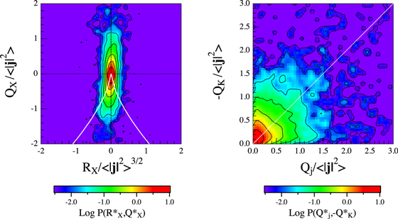
Figure 2. Joint probability distributions P(RX, QX) and P(Qj, −QK) relative to the first selected period in Table 1. The white lines refer to the discriminant line (left panel) and to the bisector line (right panel), respectively. Here, * refers to the average squared current density normalized quantities, e.g.,  .
.
Download figure:
Standard image High-resolution imageIf we compare the observed distributions with those obtained by Dallas & Alexakis (2013) by means of DNS simulations, we can see how the P(RX, QX) distribution is very similar, while the P(Qj, −QK) shows a lower alignment along the bisector line with respect to the DNS simulations. This could be due to the fact that we deal with coarse-grained quantities that are not at the dissipation scale R = L/ηp ∼ 2.6.
Figure 3 shows the joint probability distributions P(RX, QX) obtained in the case of the other four selected intervals reported in Table 1. Some changes are observed in the distributions. In particular, we see that by increasing the ratio R = L/ηp, the distributions then show an increasing probability along the discriminant line (named Vieillefosse's tails in the fluid case). Indeed, they appear to be less cigar-like shaped at larger scales in comparison with the distribution reported in Figure 2, which is the one with the smallest R.
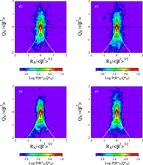
Figure 3. Joint probability distributions P(RX, QX) relative to the other selected periods reported in Table 1. The white lines refer to the discriminant line. Here, * refers to the average squared current density normalized quantities, e.g.,  .
.
Download figure:
Standard image High-resolution imageIn order to better unveil the relative weight of the different topological structures, we have computed the probability associated with the four quadrants. Table 2 shows the obtained results. The two most notable changes observed in the probability distributions with the ratio R are the increasing percentage of ISS topologies and the simultaneous decreasing percentage of SLS with decreasing R.
Table 2. Distribution of Topological Structures
| # | OSS | ISS | TLS | SLS |
|---|---|---|---|---|
Δ > 0, 
|
Δ > 0, 
|
Δ < 0, 
|
Δ < 0, 
|
|
| 1 | 29% | 35% | 21% | 15% |
| 2 | 32% | 37% | 16% | 15% |
| 3 | 27% | 31% | 18% | 24% |
| 4 | 31% | 28% | 20% | 21% |
| 5 | 30% | 30% | 19% | 21% |

|
29.8% | 32.2% | 18.8% | 19.2% |
Note. OSS outgoing spiral saddle, ISS ingoing spiral saddle, TLS tube-like structures, SLS sheet-like structures. The last line reports the average  values.
Download table as: ASCIITypeset image
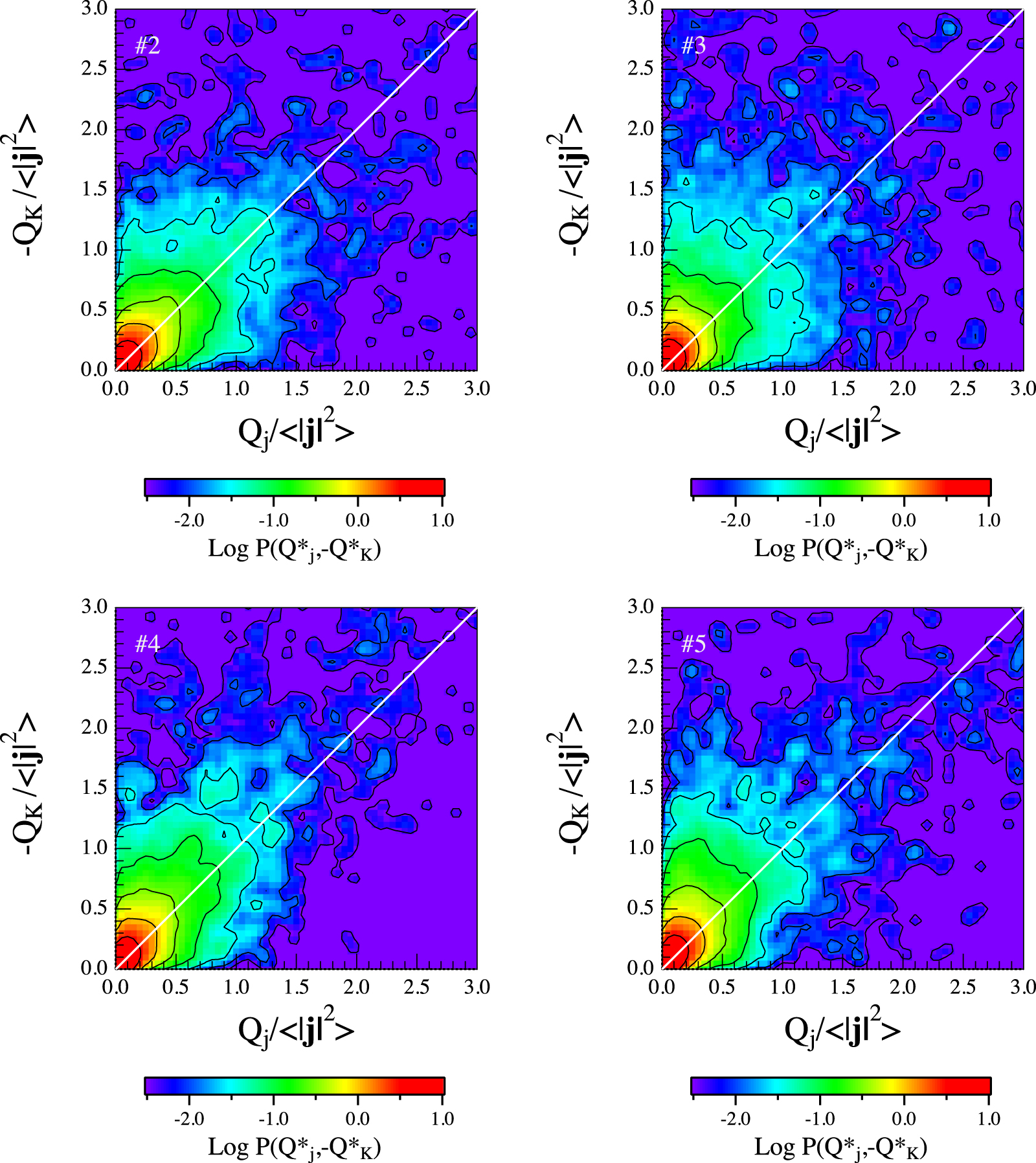
Figure 4 shows the joint probability distributions P(Qj, −QK) for the other four selected intervals reported in Table 1. As previously stated, the joint probability distribution of (Qj, −QK) provides an estimation of the energy partition into current-associated topologies and the strain magnetic configurations, quantifying the motions that participated in the ohmic dissipation. The observed P(Qj, −QK) are very similar to that reported in Figure 3 and relative to time period #1. However, they appear more aligned along the bisector line (−Qk = Qj), suggesting that ohmic dissipation in the current layers tends to increase.

Figure 4. Joint probability distributions P(Qj, −QK) relative to the other selected periods reported in Table 1. The white lines refer to the discriminant line. Here, * refers to the average squared current density normalized quantities.
Download figure:
Standard image High-resolution imageAs for the #1 interval, we evaluate the relative weights (in terms of percentage) of strain and current-associated topologies, reporting the obtained results in Table 3. We also compute the total probability contained in the cone ∣− QX − Qj ∣ ≤ 0.1Qj around the bisector line (last column in Table 3) with the aim to estimate the relevance of the current layer dissipation with the distance R from the proton inertial length ηp.
Table 3. Distribution of Dissipative Topological Structures
| # | SMT | CAT | P(∣ − QX − Qj ∣ ≤ 0.1Qj) |
|---|---|---|---|
| 1 | 63% | 37% | 6.6% |
| 2 | 61% | 39% | 8.9% |
| 3 | 70% | 30% | 7.1% |
| 4 | 67% | 33% | 8.3% |
| 5 | 66% | 34% | 9.0% |

|
65.4% | 34.6% | 8,0% |
Note. SMT strain magnetic topologies, CAT current-associated topologies. The last line reports the average  values.
Download table as: ASCIITypeset image
The percentages reported in Table 3 seem to indicate that by decreasing the characteristic scale (i.e., going toward the kinetic domain), there is then a relative increase of the energy contained in the current-associated topologies. This suggests that dissipation increases going toward the smallest scales, as expected. Conversely, the dissipation in the current layers seems to be less relevant than at larger scales. However, it is essential to note that to provide clear evidence for the above points, a more detailed and extensive analysis is required.
Another important point emerging from the analysis of the joint probability distributions P(Qj, −QK) as reported in Table 3 is the very high percentage of energy involved in strain magnetic topologies (∼65%). This result could be the counterpart of the occurrence of intermittency, which generates a multifractal structure of the dissipation field. Indeed, straining can modify the structures by pulling and stretching them so as to generate an inhomogeneous and intermittent dissipation pattern. We will return to this point later in the conclusions.
4.2. Error and Dimensionality Analysis
In the previous section, we found some interesting results. However, before tracing the conclusions of the work, it is important to investigate how reliable and robust the results are in comparison with some possible sources of error, such as noise and random fluctuations. Further, we would like to check how dissimilar the obtained distributions of invariants are when compared to those of completely random signals, i.e., without any significant correlation between the four different measurements.
In order to check the above points, we have performed three different tests:
- 1.We have investigated the effect of adding a certain percentage of random noise to the original signals. This has been done by computing the variance (standard deviation) of each independent satellite magnetic field measurement, and successively adding a Gaussian delta-correlated noise with a standard deviation equal to 1, 2, 5, and 10% of the actual signals;
- 2.We have studied the effect of randomly shuffling the measurements relative to each signal. This test should show the effect of breaking the internal correlation present in each time series, checking the robustness of stating a real correlation in the data;
- 3.We have studied the probability distribution for pure random noise signals. This has been done by generating Gaussian random noise signals of the same variance and length of the actual measurements. We have also investigated the effect of dimensionality of the random field by modifying the variances of the surrogate Gaussian signals in the different directions.
In this error analysis, we focus on the joint probability distributions P(RX, QX) as being the most sensitive. We have also checked the effects of the three tests for the probability distributions P(Qj, −QK). However, in this case, the observed changes are not as informative as those observed in P(RX, QX).
Figure 5 shows the effect of adding a different level (0.01σ, 0.02σ, 0.05σ, and 0.10σ) of Gaussian delta-correlated noise to the actual measurements of the magnetic field from the Cluster spacecraft during time interval #1 of Table 1. The effect of adding noise would return a larger spreading of the probability distribution P(RX, QX) in the plane (RX, QX) and in a clear modification of the cigar-like shape toward a shape showing a probability enhancement along the discriminant line. This could be due to the fact that large noise level could break the correlation between different satellite measurements, which could turn into a break of the cigar-like shape. If this interpretation is correct, we should observe a similar effect by shuffling the actual magnetic field time series measured by the Cluster spacecraft.
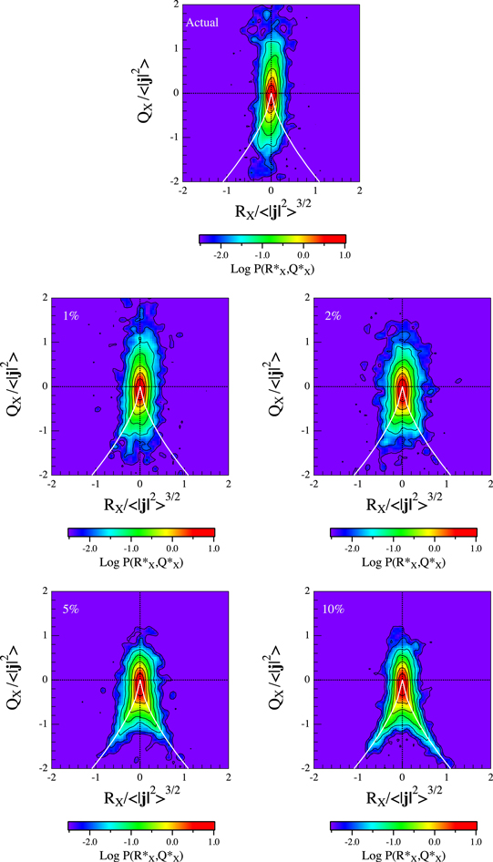
Figure 5. Comparison between the actual probability P(RX, QX) relative to the time interval #1 and that obtained adding a certain percentage (1%, 2%, 5%, and 10%) of Gaussian delta-correlated noise.
Download figure:
Standard image High-resolution imageFigure 6 shows the results of the shuffling test by comparing the actual probability P(RX, QX) and that obtained by shuffled data for time interval #1 reported in Table 1. The effect of shuffling data returns in a breaking of the cigar-like shape, which is the consequence of the breaking of spacetime correlations. We may note how the effect of data shuffling is very similar to that of adding a level of noise contained between 2% and 5%.

Figure 6. Comparison between the actual probability P(RX, QX) relative to time interval #1 and that obtained by shuffling the actual Cluster magnetic field measurements.
Download figure:
Standard image High-resolution imageThese two tests suggest that the observed structure of probability P(RX, QX), which manifests in a cigar-like shape, is due to the presence of a real spacetime correlation between the different magnetic field time series measured by the Cluster spacecraft. In other words, we could say that the cigar-like shape contains real information on the different magnetic field topological structures. Furthermore, the behavior with increasing R could be due to the breaking of the internal correlation, i.e., to a decreasing relevance of coherent magnetic field structures.
As a last point, we check the shape of the probability distribution P(RX, QX) for a completely random signal, comparing it with the actual P(RX, QX) relative to time interval #1. This study is done for a signal with different dimensionality. In particular, we generate Gaussian noise signals characterized by two and three dimensions. This is obtained by modulating the variance (standard deviation) of the surrogate vector measurements in one direction. For the 3D surrogated vector signal, the standard deviation is chosen to be the same in all three directions, while for the 2D, the variance is reduced by a factor of 10 in one direction.
Figure 7 shows the comparison of the actual probability P(RX, QX) relative to time interval #1 and those relative to 2D and 3D Gaussian delta-correlated noise. There is a clear difference between the shape of the probability P(RX, QX) of actual measurements and surrogated signals. In particular, neither the 2D nor the 3D simulated P(RX, QX) show the cigar-like shape of the actual P(RX, QX) relative to time interval #1. However, we note that the shape of the 2D simulated P(RX, QX) resembles the one observed in the case of time intervals #4 and #5, which are characterized by large values of R. This similarity could suggest that there is an evolution of the topological dimension of the structures along the inertial range. In other words, going from large to small scales, the turbulence seems to acquire a more 3D nature, while the large scales are compatible with a more 2D character of the fluctuation field. In passing, we also note that the shape of the 3D simulated probability is very similar to the one obtained by shuffling the actual measurements (see Figure 6).

Figure 7. Comparison between the actual probability P(RX, QX) relative to time interval #1 and that obtained by Gaussian delta-correlated noise with a different dimensionality.
Download figure:
Standard image High-resolution image
5. Summary and Conclusions
In this work, we have presented a characterization of the 3D magnetic topological structures involved in space plasma turbulence at different scales in the inertial range by investigating the statistics of the invariants of the coarse-grained magnetic filed gradient tensor for a set of five solar wind intervals. To our knowledge, this is the first attempt in using the TETRAD method to obtain information about the magnetic topological structures involved in turbulence.
Our main results can be summarized as follows:
- 1.The joint probability P(RX, QX) shows a clear dependence on the scale in the inertial range (and, in particular, on the distance from the proton inertial scale), as monitored by the ratio R = L/ηp;
- 2.The observed scale-dependence seems to also be consistent with a change in the dimensionality of the fluctuation field from quasi-2D at large scales and nearly 3D at small scales near the proton inertial length ηp;
- 3.The joint probability P(Qj, −QK) suggests that at small scales, i.e., for decreasing R, there is a relative increase of the current-associated energy. Conversely, the role of the current layer configurations for dissipation seems to become less relevant by decreasing the spatial scale.
As a result of the analysis on the topological invariants, we can conclude that the magnetic field lines are mainly elliptic, i.e., characterized by swirling lines associated with ISS/OSS topologies. Tube-like and sheet-like topologies are also present, although they are less relevant. Heating is mainly connected with dissipation in current layers and current-associated topologies.
Furthermore, we have found a strong indication of the change of the turbulence dimensionality from large scales to kinetic ones. Indeed, the results suggest that at large scales, the topological structure of the fluctuations is more consistent with a 2D scenario. This is well in agreement with previous observations of a quasi-2D Alfvénic component in the solar wind turbulence (see, e.g., Petrosyan et al. 2010, and references therein). However, due to the straining motions, which seem to be a relevant ingredient at all of the investigated scales (∼65% of energy) and can pull and stretch the magnetic topologies, the quasi-2D large-scale structure of the magnetic field topologies is modified so as to generate a more isotropic 3D turbulent field at the smallest scales. On the other hand, the fact that a large part of the energy is associated with straining motions is also in agreement with the occurrence of a quasi-Kolmogorov −5/3 spectrum of magnetic and velocity field fluctuations (refer to Zhou et al. 2004, and references therein). As a secondary effect, the modification and the fragmentation of the magnetic topologies from a quasi-2D to a nearly 3D field at the kinetic scales could also be responsible for the high degree of spatial complexity of the magnetic field at the smallest scales, which involves the formation of small-scale localized current sheets. The observed changes have been associated with the occurrence of strain motions, which may cause the nonlinear self-stretching of the structures generating large intermittent fluctuations at small scales. As underlined in Zhou et al. (2004), this is a fundamental feature of MHD turbulence, which is related to nonlinear strain-type motions, which, we believe, can also be at the origin of the occurrence of intermittency.
Clearly, more work is necessary to investigate what happens at the kinetic scales, i.e., below the ion (proton) inertial scale where dissipation might occur. With respect to this point, we believe that the study of small-scale magnetic field structure topologies could benefit from the recent measurements by the NASA-MMS mission once the methodology discussed here is applied. The construction of a self-consistent stochastic dynamical system describing the time evolution of the coarse-grained topological invariants and of the gradient tensors, ∂iuj and ∂ibj, and its numerical implementation is going to be the next challenge in the description of MHD turbulent structures' evolution.
We thank the ESA Cluster Science Archive (https://www.cosmos.esa.int/web/csa) and the instrument PIs and teams for providing the data used in this work. The research leading to these results has received partial funding from the Italian Space Agency under grant agreement No. ASI-INAF 2015-039-R.O. "Missione M4 di ESA: Partecipazione Italiana alla fase di assessment della missione THOR." V.Q. thanks the Italian Space Agency (ASI) for the financial funding under contract ASI "LIMADOU Scienza."