


Abstract
Numerical simulations of 1D force-free magnetodynamics (FFMD) by Koide and Imamura showed details of the energy extraction mechanism around a rapidly spinning black hole under the force-free condition in the case of a radial magnetic surface along the equatorial plane. The energy is transported like a tsunami from the ergosphere and spreads to the outside. In this paper, we perform 1D FFMD simulations with nonradial magnetic surfaces along the equatorial plane, which are more general magnetic surface configurations. Using the results of simulations and analytic solutions of the steady-state force-free magnetic field, we find that, except in the case of a radial magnetic surface at infinity, the tsunami induced at the neighborhood of the horizon damps gradually and energy flux along the equatorial plane vanishes after a long period of time or at infinity. This suggests the energy extracted from the spinning black hole through the nonradial magnetic field is transported toward the high latitude around the axis of the black hole and is converted to the kinetic energy of the jet or outflow.
Export citation and abstract BibTeX RIS
1. Introduction
High-energy phenomena related to black holes are observed throughout the universe, such as relativistic jet formation in active galactic nuclei (AGNs; Pearson & Zensus 1987; Biretta et al. 1999), micro-quasars (black hole binaries; Mirabel & Rodriguez 1994; Tingay et al. 1995), and gamma-ray bursts (GRBs; Kulkarni 1999). These relativistic jets are thought to form via drastic phenomena in the accretion disks in the vicinity of black holes (Meier et al. 2001; Levinson 2006). Recent general relativistic magnetohydrodynamics (GRMHD) studies with the ideal magnetohydrodynamic (MHD) conditions of plasma around a black hole suggested that relativistic jets from AGNs are driven by energy extracted from the spinning black hole (Koide et al. 2006; McKinney 2006). The team of the Event Horizon Telescope (EHT) collaboration has reconstructed images of the shadow of the supermassive black hole in the center of the giant elliptical galaxy M87. They have compared the single, high-quality EHT data to a library of images produced from GRMHD simulations by general relativistic ray-tracing calculations (Porth et al. 2019; The Event Horizon Telescope Collaboration 2019). With the comparison, they concluded that there is a strong energy flux directed away from the poles of the black hole, and that this energy flux in the central engine for the M87 jet is powered by the extraction of free energy associated with black hole spin.
Several mechanisms for extracting the rotational energy of black holes have been proposed, for example, the Penrose process, the Blandford–Znajek mechanism, the MHD/magnetic Penrose process, and the superradiance (Penrose 1969; Press & Teukolsky 1972; Teukolsky & Press 1974; Blandford & Znajek 1977; Takahashi et al. 1990; Hirotani et al. 1992; Koide et al. 2002; Koide 2003). The Penrose process, one of these proposed mechanisms, has a simple and clear explanation in that it extracts energy from the rotational energy of dropping fission-separated particles with negative energy. However, it is hard to explain the relativistic jet formation by this process primarily because the process accelerates the particles perpendicular to the axis of the spinning black hole. The Blandford–Znajek mechanism, which is a mechanism to extract energy via magnetic fields, is most promising for an engine for relativistic jets. We tried to explain the Blandford–Znajek mechanism by the negative electromagnetic energy-at-infinity density like the Penrose process (Koide et al. 2006; Koide & Baba 2014). However, Toma & Takahara (2016) correctly pointed out the sign of the energy-at-infinity density is opposite in the ergosphere with the Boyer–Lindquist and Kerr–Schild coordinates. Then the intuitive explanation of the Blandford–Znajek mechanism by the negative electromagnetic energy-at-infinity density is implausible. To find an alternative intuitive explanation of the Blandford–Znajek mechanism, we expect that the time evolution of the electromagnetic field around a spinning black hole using the force-free magnetodynamics (FFMD) is helpful. Numerical simulations of the FFMD in axisymmetry with initial conditions of split monopole field and vertically uniform magnetic field had been performed (Komissarov 2001; Komissarov & McKinney 2007). They showed not only the time evolution of the magnetic surface but also the energy extraction from the spinning black hole due to the magnetic field. However, their analysis of the time evolution of the electromagnetic field was not enough and no intuitive explanation of the energy extraction mechanism was shown. Koide & Imamura (2018) performed one-dimensional force-free magnetodynamic (1D-FFMD) simulations to show a detailed process for the extraction of the rotational energy from a rapidly spinning black hole in the case of radial magnetic surface. They analyzed the numerical results of 1D-FFMD simulations in detail to show the intuitive explanation of the Blandford–Znajek mechanism. In the neighborhood of the horizon, called the "stretched horizon," the energy flux P, the total current I, and the angular velocity of the magnetic field lines ΩF are independently induced at each point due to the frame-dragging effect. The continuity of the electromagnetic field with the Kerr–Schild coordinates at the stretched horizon yields the relation between I and ΩF. The condition at the stretched horizon behaves as a source of the energy flux, but not a source of the energy itself. The condition at the stretched horizon was derived by Znajek (1997) and is called the "Znajek condition." The energy comes from the inside of the black hole, as indicated by the profile of the energy flux. Beyond the stretched horizon, the energy is transported like a "tsunami" and spreads outward toward infinity. Even the degeneracy of the force-free condition, which induces the electromagnetic wave (tsunami) in the ergosphere, is sustained by the Znajek condition at the stretched horizon (Koide & Imamura 2018). The tsunami smoothly propagates outward to infinity when the initial background magnetic field is radial. The above detailed analysis of the 1D-FFMD simulation results has clarified the intuitive process of the energy extraction from the black hole through the magnetic field around the horizon.
In this paper, we investigate the energy transport from a spinning black hole when we assume various shapes of magnetic surfaces along the equatorial plane such as the "incurvature-flared" magnetic surface and the "excurvature-flared" magnetic surface. The cross section of the incurvature-flared magnetic surface is similar to that of the petal of a tulip (Figure 1, middle panel) and the cross section of the excurvature-flared magnetic field is similar to that of the petal of a lily (Figure 1, right panel), whose mathematical definitions are shown in Section 2. In the case of the incurvature-flared magnetic surface, P, I, and ΩF take a very long time to propagate outward toward infinity. It is required to adjust for the discrepancies with respect to P, I, and ΩF at the ergosphere and infinity. With respect to P, because the steady-state solution is P = 0, energy is not stably emitted from the spinning black hole. In the case of an excurvature-flared magnetic surface, P, I, and ΩF never reach the steady state where the energy flux P = 0. These results indicate that the electromagnetic energy is transported toward infinity along the magnetic field along the equatorial plane only in very special cases, where the magnetic surface is radial. At infinity, the radial magnetic field along the equatorial plane of the black hole is improbable because there is no magnetic monopole. Then, in most cases, the electromagnetic energy extracted from the spinning black hole through the magnetic field is transported toward infinity except to the direction parallel to the equatorial plane. It suggests that the electromagnetic energy from the black hole is concentrated between the axis and the middle latitude at infinity and the jet or outflow is produced when the electromagnetic energy is converted to the kinetic energy of plasma.

Figure 1. Flux coordinates for the 1D FFMD simulation with the three different types of magnetic surfaces along the equatorial plane around a spinning black hole. We assume that the electromagnetic field is force-free and axisymmetric with planar symmetry with respect to the equatorial plane. The left panel shows the radial magnetic surface; the middle panel shows the incurvature-flared magnetic surface; and the right panel shows the excurvature-flared magnetic surface.  in these panels indicates the magnetic field lines.
Download figure:
Standard image High-resolution imageIn Section 2, we show the basic equations for an arbitrary magnetic surface configuration and the method for the numerical calculations. In Section 3, we present the analytical solutions of the 1D steady-state electromagnetic field around a spinning black hole under the force-free condition. In Section 4, we show the numerical results for three types of magnetic surface configurations (radial, incurvature-flared, and excurvature-flared) to compare the numerical results to the steady-state solutions. In Section 5, we discuss the interpretation of the numerical results with respect to the three types of magnetic configurations.
2. Method of 1D FFMD
2.1. Basic Equations of FFMD and 1D-FFMD
In this section, we review the basic equations of the FFMD and show the 1D-FFMD equations. The equations are based on the force-free condition and Maxwell's equations (Komissarov 2001, 2004). We use a coordinate system  , where the line element is written as
  . The Greek character of subscripts runs from 0 to 3, and the Roman character of subscripts runs from 1 to 3. As a unit system, we set the speed of light c = 1, the gravitational constant G = 1, the vacuum permittivity, and the permeability
  0 = 1, μ0 = 1, respectively. Furthermore, the mass of a black hole is set to M = 1 in this paper.
The general relativistic covariant Maxwell's equations are


where ∇μ is the covariant differential,  is the electromagnetic field-strength tensor,
  is the dual tensor of
  , and
, and  is the four current density (ρe is the electric charge density).
  is the Levi–Civita tensor, which is defined as
  .
.  is the totally asymmetric symbol defined as
  if the order
 ![$[\mu \nu \rho \sigma ]$](https://content.cld.iop.org/journals/0004-637X/878/1/4/revision1/apjab1d57ieqn12.gif) is an even permutation of [0123],
is an even permutation of [0123],  if the order
 ![$[\mu \nu \rho \sigma ]$](https://content.cld.iop.org/journals/0004-637X/878/1/4/revision1/apjab1d57ieqn14.gif) is an odd permutation of [0123], and
is an odd permutation of [0123], and  unless
  , and σ are all different. g is the determinant of
  . The electric field Eμ and the magnetic field Bμ are, respectively, given by


Maxwell equations yield the law of conservation of energy–momentum,

where  is the four electromagnetic energy–momentum tensor and
  is the four Lorentz force density. Using the force-free condition
  , we have

For the numerical calculations of 1D-FFMD, we use Equation (6) instead of (1) to avoid the explicit calculation of Jμ.
In this paper, we use Kerr–Schild coordinates to calculate the electromagnetic field inside the black hole. The metric of Kerr–Schild coordinates  around a spinning black hole, whose mass is M and spin parameter
  (J is the angular momentum of the black hole), is given by
where  ,
,  ,
,  , and
, and  =
= 
 with
with  . In this coordinate system, we have the shift vector
  ,
,  ,
,  and the lapse function
  where the lapse function and the shift vector are defined as
  ,
,  , respectively. The determinant of (γij) (γij is the spatial component of the metric tensor) is
  ,
,  , and
, and 
Here, we introduce a new coordinate system for the 1D-FFMD of the electromagnetic field at the equatorial plane around a black hole. We assume the magnetic surface is axisymmetric with respect to the spin axis of the black hole, and symmetric with respect to the equatorial plane and the axisymmetric magnetic surface is stationary. In such cases, the azimuthal component of the vector potential  is stationary. We use Ψ as the colatitude coordinate instead of θ. Now we define the new coordinate system
  called the "flux coordinates" (see Figure 1). In the flux coordinate system, the axisymmetric magnetic surface is given by
  = const ≡ Ψ0. We set Ψ as x2 = Ψ0 indicates the equatorial plane. In the flux coordinates, we have BΨ = 0 obviously.
To introduce the 3+1 formalism of the 1D-FFMD equations, we use the local frame called the "normal observer frame"  as
as

Using the quantities of the normal observer frame and the conditions  and ∂/∂ ϕ = 0, we derive the 3+1 formalism of the 1D-FFMD equations according to Equations (2) and (6) (see Section 2, Appendix A, and B in Koide & Imamura 2018):


where  is the four velocity of the normal observer frame,
  is always zero in Kerr–Schild coordinates.
  is always zero on the equatorial plane.
  and
and  are the electromagnetic energy density and the Poynting flux density measured by the normal observer, respectively.
Equation (9) gives  , where B0 is constant (B0 = 1). The poloidal component of the magnetic field
  is given as
  .
.
In the 1D-FFMD simulations, we need to calculate  using
using  , and
, and  . We use the relationship

where  ,
,  ,
,  , and
, and  . We also used
  derived from the force-free condition (see Appendix B in Koide & Imamura 2018). We have JΨ = 0 on the equatorial plane. We also use


In the numerical calculations of the 1D-FFMD, we calculate  using Equations (16) and (17) in spite of Equation (12), which is the time development of the energy density.
Using the flux coordinate system (r, Ψ, ϕ), magnetic surface configurations around the main magnetic surface along the equatorial plane (Ψ = Ψ0) is given by  , where H(r) is a function of r, which describes the flare shape of the cross section of the magnetic surfaces beside the equatorial plane. When H(r) becomes finite in the limit of
  , the magnetic field is asymptotically radial (Figure 1, left panel). When H(r) becomes zero in the limit of
  , the magnetic field is similar to the cross section of a tulip petal, which we call an "incurvature-flared magnetic surface" (Figure 1, middle panel). When H(r) becomes infinite in the limit of
  , the magnetic field is similar to the cross section of a lily petal, which we call an "excurvature-flared magnetic surface" (Figure 1, right panel). In this paper, we set
A magnetic surface given by m = 0 is radial. A magnetic surface with m = 1 at infinity is that of a magnetic quadrupole imaginarily located at the center position of the black hole. In this paper, we use m = 0, m = −0.25, and m = 0.25, which correspond to radial, incurvature-flared, and excurvature-flared magnetic surfaces, respectively. In the cases of an incurvature-flared and an excurvature-flared magnetic surfaces, we set H(r) = 1 in the vicinity of the horizon. The coefficient rp is a parameter adjusting the region of vending of the magnetic surface  . In this paper, we set rp = 0.25, which indicates that a magnetic surface is radial in the region
  . It is noted that Equation (18) yields B0 = 1. This means we normalize the magnetic field strength as B0 = 1 when we use Equation (18).
2.2. Method of Numerical Calculation
We used the Lax–Wendroff scheme in the numerical calculations of the 1D FFMD. The mesh number of the standard case is 10,000 (if necessary, we set the larger-mesh number 50,000 and 100,000). We perform the simulations in the range  (
( ,
,  , 1000M, or 2000M). The test numerical calculations and extended forms of the 1D-FFMD are shown by Koide & Imamura (2019, in preparation).
3. Constants of Steady State of 1D-FFMD
We provide analytical solutions with conservation constants of the steady state of the 1D-FFMD. We assume that the electromagnetic field is stationary, axisymmetric, and planar symmetry with respect to the equatorial plane. First, the law of the conservation of energy is (See Appendix C in Koide & Imamura 2018)

where  is the electromagnetic energy-at-infinity density and
  is the electromagnetic energy flux density (χμ = (1, 0, 0, 0) is the time-symmetry transformation Killing vector). Thus, the energy flux is given by


In the case of a steady state, the right-hand side of Equation (10) vanishes and we obtain a constant C

Using the constant B0 and C, we have a constant

ΩF is the angular velocity of the magnetic field lines. Finally, Equation (11) with JΨ = 0 derived from the force-free condition yields a constant of the total current

Equations (21), (23), and (24) yield the relationship as follows

We drive steady-state solutions for an arbitrary spin parameter a* on the equatorial plane. I and ΩF yield the azimuthal component of the magnetic field and the Ψ component of the electric field, respectively


Subsequently, we present the relationship between I and ΩF in an arbitrary spin parameter a*. We can apply the special relativistic solution of the force-free electromagnetic wave at infinity (r ≫ M) because we assume that the space (r, Ψ, ϕ) becomes orthogonal at infinity. That is, the force-free electromagnetic field at infinity satisfies

where o represents the variables observed at the orthonormal coordinates of the normal observer frame. Equation (28) becomes  on the equatorial plane. Thus, we have

where  is the value of H(r) at infinity.
We have  at the vicinity of the horizon because we assume the radial magnetic surface at the vicinity of the horizon. The denominators of the right-hand sides of Equations (26) and (27) vanish at the horizon. The continuous condition of
  and
and  at the horizon yields
  . Using Equation (29) and
  , we obtain

where  . Equations (25), (29), and (30) yield I and P as follows, respectively:


This is the generalization of the solution at the equatorial plane given by Menon & Dermer (2005) who assumed the radial magnetic field of the monopole. It is noted that P vanishes when  or
or  . In such a case, no energy is stably emitted from a spinning black hole.
Here, we show the analytic solutions of P, I, and ΩF of the steady-state solution with a spin parameter a* = 0.95 in cases of three types of the magnetic surfaces given by Equation (18). In the case of a radial magnetic surface (m = 0), we have  . Thus, we find the steady-state solution is given by P = 0.048, I = −0.129, and
  according to Equations (30)–(32) In the case of an incurvature-flared magnetic surface (m = −0.25), we have
  . Thus, we find the steady-state solution is given by P = 0, I = −0.554, and ΩF = 0 according to Equations (30)–(32). In the case of an excurvature-flared magnetic surface (m = 0.25), we have
  . Thus, we find the steady-state solution is given by P = 0, I = 0, and ΩF = 0.363 according to Equations (30)–(32). For the excurvature-flared magnetic surface, the magnetic field lines with I = 0 are straight. When r is larger than c/ΩF, the velocity of the azimuthal of the magnetic field lines is beyond the speed of light. If we assume the ideal MHD conditions, the velocity of the plasma which moves with the magnetic field lines is more than the speed of light. It is noted that we do not necessarily have to consider the ideal MHD conditions and we otherwise use the resistivity MHD conditions. If we assume the resistivity MHD conditions, we have no force that drives the rotation of the straight magnetic field lines. In any case, the steady-state solution is never realized in the case of an excurvature-flared magnetic surface.
4. Results of the 1D-FFMD Numerical Simulations
We show the numerical test results of 1D-FFMD simulations of the electromagnetic field for the three types of the axisymmetric magnetic surfaces: radial, incurvature-flared, and excurvature-flared.
4.1. Case of a Radial Magnetic Surface
We performed numerical 1D-FFMD simulations of a force-free magnetic field in the radial magnetic surface around a spinning black hole with a spin parameter a* = 0.95 (Koide & Imamura 2018). The initial conditions of the simulation are given by P = 0, ΩF = 0, and  around the black hole. Figure 2 shows the time evolution of P, I, ΩF, and
  . P and ΩF start to rapidly increase around the ergosphere to the value expected by the analytical steady-state solution (the horizontal dashed–dotted line). The region with nearly steady-state values of P and ΩF spreads outward like a tsunami from the region around the ergosphere at the speed of light (t = 100M) and P and ΩF finally converge to the expected steady-state solution over the entire calculation region (r ≤ 100) (t = 200M). I also converges to the steady-state solution. Note that
  in the vicinity of the ergosphere is positive. A more detailed analysis of the numerical results for a radial magnetic surface is given in Koide & Imamura (2018).

Figure 2. 1D-FFMD simulation with initially zero power and angular velocity of the magnetic field lines (P = 0, ΩF = 0) for a radial magnetic surface around a rapidly spinning black hole (a* = 0.95). In this case, the initial electric field in the normal frame is zero ( ). The dashed lines show the quantities at t = 0. The dotted lines show the results at t = 100M. The solid lines show the results at t = 200M. The horizontal dashed–dotted lines show the analytical values of the steady state, and the vertical dashed–dotted lines show the horizon of the spinning black hole. The values of P, I, and ΩF at t = 200M are nearly the same as the corresponding values for the analytical steady-state solution.
Download figure:
Standard image High-resolution image4.2. Case of an Incurvature-flared Magnetic Surface
We show the numerical results for an incurvature-flared magnetic surface around a spinning black hole with a* = 0.95. The incurvature-flared magnetic surface is given by m = −0.25 in Equation (18). The initial conditions of the force-free electromagnetic field are given by P = 0,  , and
, and  . Figure 3 shows the time evolution of P, I, ΩF, and
  . P and ΩF start to rapidly increase around the ergosphere, as shown in the case of a radial magnetic surface. However, the region of finite P and ΩF spreads outward relatively slowly and appears to not converge to the values of the steady state like a tsunami (t = 100M, 200M). The region of finite I also spreads outward but does not rapidly converge to the value of the steady state.
  is positive over the entire calculation region.
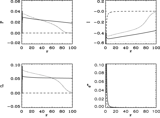
Figure 3. Similar to Figure 2 but for the case of an incurvature-flared magnetic surface. In this case, the initial electric field in the normal frame is zero ( ). The dashed lines show the quantities at t = 0. The dotted lines show the results at t = 100M. The solid lines show the results at t = 200M. The horizontal and vertical dashed–dotted lines are the same as those in Figure 2. The values of P, I, and ΩF at t = 200M have not reached the values of the analytical steady-state solution.
Download figure:
Standard image High-resolution imageTo investigate the time evolution of the field for the incurvature-flared magnetic surface in the long term after t = 200M, we show the result at t = 1000M in Figure 4. P, I, and ΩF gradually approach the values expected by the steady-state solution: P = 0, I = 0.554, and ΩF = 0. The magnetic surface near the horizon is nearly radial because H(r) = 1 at the horizon; therefore, the local condition at the horizon causes P to increase. However, in the steady state, P is expected to vanish far from the black hole. It takes a very long time to reach the steady-state solution to adjust for this discrepancy. After a very long time, the steady state given by P = 0, I = 0.554, and ΩF = 0 is realized via outward propagation and reflection. Finite I indicates that the magnetic field lines are twisted spirally while no energy is emitted from the spinning black hole (P = 0) in the case of an incurvature-flared magnetic surface,  .
.

Figure 4. Similar to Figure 3 but for a much longer-term result for the case of the incurvature-flared magnetic surface. The dashed lines show the quantities at t = 0. The dotted lines show the results at t = 500M. The solid lines show the results at t = 1000M. The horizontal and vertical dashed–dotted lines are the same as those in Figure 2. The values of P, I, and ΩF are approaching the steady-state solution very gradually, as shown by the lines at t = 1000M.
Download figure:
Standard image High-resolution image4.3. Case of an Excurvature-flared Magnetic Surface
We show the numerical results for an excurvature-flared magnetic surface (m = 0.25) around a spinning black hole with a* = 0.95. The initial conditions are given by P = 0, ΩF = 0, and  around the black hole. Figure 5 shows the time evolution of P, I, ΩF, and
  . The regions of finite P and ΩF spread outward gradually but differ from the case of a radial magnetic surface (t = 100M). P and ΩF do not converge to the value of the steady-state solution (t = 200M). Beyond the ergosphere, I also increases outward but does not converge to the steady-state value.
  again has a positive value over the entire calculation region.

Figure 5. Similar to Figure 3 but for the case of an excurvature-flared magnetic surface. The dashed lines show the quantities at t = 0. The dotted lines show the results at t = 100M. The solid lines show the results at t = 200M. The horizontal and vertical dashed–dotted lines are the same as those in Figure 2. The values of P, I, and ΩF at t = 200M have not reached the values of the analytical steady-state solution.
Download figure:
Standard image High-resolution imageWe investigated the time evolution of the fields in the excurvature-flared magnetic surface in the long term. As shown in Figure 6, even at t = 2000M, P, I, and ΩF do not reach the values expected by the steady-state solution: P = 0, I = 0, and ΩF = 0.363. This nonconvergence is explained by the discrepancy between the local condition at the horizon (P > 0) and the steady state (P = 0), as mentioned in the last paragraph of Section 3. Finite ΩF with I = 0 is the steady state in the case of an excurvature-flared magnetic surface;  indicates that the straight magnetic field lines rotate while no energy is emitted from the spinning black hole (P = 0).

Figure 6. Similar to Figure 5 but for a much longer-term result for the case of an excurvature-flared magnetic surface. The dashed lines show the quantities at t = 0. The dotted lines show the results at t = 1000M. The solid lines show the results at t = 2000M. The horizontal and vertical dashed–dotted lines are the same as those in Figure 2. P, I, and ΩF do not reach the constant values of the steady-state solution even at t = 2000M.
Download figure:
Standard image High-resolution image
Using the 1D-FFMD numerical simulations of the three types of magnetic surfaces, we conclude that no energy is radiated in a stationary manner from the spinning black hole except in the case of a radial magnetic surface at infinity. A radial magnetic surface at infinity is given by finite  (
( ), while in the case of an excurvature-flared magnetic surface
  , even after an extremely long term the numerical solution does not converge to the steady state.
5. Discussion
We presented 1D-FFMD simulations of the spontaneous energy radiation from a rapidly spinning black hole (a* = 0.95) under the conditions of radial, incurvature-flared, and excurvature-flared magnetic surfaces. In the case of a radial magnetic surface, the region of finite electromagnetic energy flux P, which is initially zero over the calculation region, spreads outward like a tsunami at the speed of light. After a certain amount of time (t = 200M), this tsunami with a constant P converge to the steady-state solution given by Equation (28). The transient process with the tsunami behavior has also been demonstrated in 2D–FFMD simulations by Komissarov (2001). It appears that the source of P exists in the ergosphere. As shown in the detailed analyses given by the 1D-FFMD simulations (Koide & Imamura 2018), this energy radiation is caused by the Znajek condition and the degeneracy (magnetic field dominated) of I and ΩF at the stretched horizon. In the cases of incurvature-flared and excurvature-flared magnetic surfaces, the region of finite P, which is initially zero, gradually spreads outward. In the case of an incurvature-flared magnetic surface, P converges to the expected steady-state solution after very long times (t = 1000M). In the case of an excurvature-flared magnetic surface, the force-free electromagnetic field has no tendency to converge to the steady state. In this case, it appears that the steady state never appears.
Here, we discuss the reasons for slow or no convergence in the cases of incurvature-flared and excurvature-flared magnetic surfaces, respectively. The relations between I and ΩF at infinity are


In the case of an incurvature-flared magnetic surface, we have  at infinity. Because I should be finite and ΩF vanishes at infinity according to Equation (33). Therefore,
  at infinity according to Equation (34). In the case of an excurvature-flared magnetic surface, we have
  at infinity. Then, I vanishes and ΩF becomes finite at infinity according to Equation (33) and
  is zero according to Equation (34). In either case, we obtain P = 0 at infinity. Conversely, P is greater than zero near the horizon in the early stage because the magnetic surfaces are radial in all cases. It is noted that in the radial magnetic field case the tsunami of the force-free wave is caused around the ergosphere and propagates outward smoothly. The detailed process of the tsunami induction in the ergosphere is shown in Koide & Imamura (2018). Therefore, there is a contradiction for values of P at the stretched horizon and steady state. It is easy to imagine that it takes a very long time to converge to the steady state due to adjusting for this discrepancy. Finally, the value of P in the numerical simulation decreases and vanishes as expected for the steady-state analytic solution in the case of an incurvature-flared magnetic surface. In the steady state with P = 0, the outward propagation and the inward reflection are balanced so that the total energy flux vanishes. On the other hand, in the case of an excurvature-flared magnetic surface, it appears that the electromagnetic state does not converge to the steady state. In the steady state with an excurvature-flared magnetic surface, I is expected to vanish while ΩF is finite. This indicates that the straight magnetic field lines rotate with finite angular velocity ΩF. At a certain distance (c/ΩF ∼ 2.75M) from the black hole, the magnetic field lines rotate faster than the speed of light, which is impossible, as mentioned in the last paragraph of Section 3. Therefore, in the case of an excurvature-flared magnetic surface, the electromagnetic field will not converge to the steady state. In conclusion, only for a radial magnetic surface at infinity does a spinning black hole radiate electromagnetic energy in a stationary manner along the equatorial plane. In the cases of incurvature-flared and excurvature-flared magnetic surfaces, the energy is not emitted stably. This indicates that a spinning black hole does not emit electromagnetic energy through the magnetic field lines along the equatorial plane except for the very special magnetic configuration like the radial magnetic field. In astrophysical situations, the radial magnetic field around the equatorial plane of the black hole is improbable at infinity because there is no magnetic monopole. The energy extracted from the spinning black hole is expected to be supplied to the region around the axis at infinity and the jet or outflow is caused.
It is noted that van Putten (1999, 2001) and van Putten & Levinson (2003) considered the black hole–torus system as the progenitor of the inner engine of GRBs. When we consider the corresponding situation along the main magnetic surface at the equatorial plane, the outer boundary located at a finite point should be assumed. At the early stage, the tsunami is caused from the ergosphere and spreads outward along the radial magnetic field until it reaches the boundary. It is subsequently reflected by the outer boundary. This reflected wave complicates the electromagnetic field between the ergosphere and the boundary. This complex process will be investigated further in terms of 1D-FFMD simulations.
In this paper, we considered the 1D axisymmetric force-free electromagnetic field along the main magnetic surface at the equatorial plane, where the magnetic flux surfaces are assumed to be of three types, radial, incurvature-flared, and excurvature-flared. On the other hand, Blandford & Znajek (1977) obtained the analytic solutions of 2D axisymmetric force-free field in the steady state around a very slowly spinning black hole (a* ≪ 1), which are called the Blandford–Znajek solutions. The radial (split monopole) and paraboloidal magnetic field configurations (Ψ = Ψ0(r, θ)) are employed as the zeroth-order field with respect to a*. The method of 1D-FFMD is generalized for an arbitrary axisymmetric main magnetic surface (S. Koide & T. Imamura 2019, in preparation) from the main magnetic surface along the equatorial plane in the paper. Using the generalized 1D-FFMD method, we obtain the expressions of the Blandford–Znajek solutions identical with Equations (6.5) and (7.5) in Blandford & Znajek (1977) for the radial and paraboloidal magnetic field cases, respectively.
As future work, we need to analyze the reflection of the force-free electromagnetic waves due to the adjustment for cases of incurvature-flared and excurvature-flared magnetic surfaces. We will also extend the one-dimensional numerical calculations to two-dimensional calculations in the near future.
One of the authors (S.K.) thanks Mika Koide for useful comments on this manuscript. We also thank Masaaki Takahashi and Fumio Takahara for their fruitful discussion and suggestions on this study.