


Abstract
Since polarized synchrotron intensity arising from magnetized turbulence is anisotropic along the direction of mean magnetic field, it can be used to trace the direction of the mean magnetic field. In this paper, we provide a statistical description of anisotropy of polarized synchrotron intensity. We use a second-order structure function and a new statistics, quadrupole moment (QM), at different wavelengths. The second-order structure function visualizes anisotropy of polarized intensity (PI) along the direction of mean magnetic field. Using QM, we quantify the degree of anisotropy displayed in the structure function. Since Faraday rotation, which depends on wavelength, can change the structure of PI and result in depolarization, we study how the anisotropic structure changes with wavelength. First, we consider polarized synchrotron emission arising from one spatial region, in which synchrotron emission and Faraday rotation occur simultaneously. Second, we also consider polarized synchrotron emission from two spatially separated regions. When the wavelength is very small, the observed polarization exhibits the averaged structures of both foreground and background regions. As the wavelength increases and Faraday rotation becomes important, depolarization wipes out large-scale structures, while small-scale anisotropy begins to reflect that of the foreground region, where the depolarization effect has relatively weak influence.
Export citation and abstract BibTeX RIS
1. Introduction
Plenty of observations and theoretical works have supported the fact that magnetic fields are of great importance for most astrophysical systems on a wide variety of scales, such as the interstellar medium (Elmegreen & Scalo 2004) and the intracluster medium (Ensslin & Vogt 2006). For instance, turbulent magnetic fields play leading roles in many processes, including star formation (Mac Low & Klessen 2004; McKee & Ostriker 2007), galaxy evolution, accretion flows (Balbus & Hawley 2002), astrophysical shocks, cosmic-ray propagation (Schlickeiser 2003; Longair 2011), magnetic reconnection (Lazarian & Vishniac 1999; Kowal et al. 2009; Eyink et al. 2011; Lazarian et al. 2015), and heat and mass transports (Narayan & Medvedev 2001; Lazarian 2006).
Research on polarized emission will be useful to identify magnetic structures. Relativistic electrons spiraling in magnetic fields produce synchrotron radiation, which is polarized (Ginzburg 1981). Both intensity of synchrotron emission and rotation of its polarization angle (a.k.a Faraday rotation) are related to magnetic fields. The total intensity of synchrotron emission,  , where ne is number density of relativistic electrons and the line of sight (LOS) is along the z direction, provides information about the strength of the magnetic field component perpendicular to the LOS. Faraday rotation is sensitive to the LOS magnetic field and thermal electron number density, and proportional to wavelength squared:
  , where δϕ is rotation of the polarization angle. The integral in the expression is called the rotation measure (RM):
  . Therefore, we can estimate the properties of the magnetic field from polarization of synchrotron emission and Faraday rotation (Waelkens et al. 2009; Junklewitz & Ensslin 2011).
When the magnetic field in a turbulent medium is sufficiently strong, turbulence structures tend to be anisotropic (Shebalin et al. 1983; Goldreich & Sridhar 1995; Lazarian & Vishniac 1999; Cho & Vishniac 2000; Maron & Goldreich 2000; Kowal & Lazarian 2010; Brandenburg & Lazarian 2013). The study of anisotropic structure is essential for prehension of the properties of the magnetized turbulent medium where the polarization occurs. The theory of incompressible magnetohydrodynamic (MHD) turbulence that was formulated by Goldreich & Sridhar (1995, henceforth GS95) predicts scale-dependent anisotropy of eddies with the degree of anisotropy increasing as the eddy size gets smaller. The deficiency of the original formulation of GS95 theory was that this anisotropy was considered in the reference frame of the mean magnetic field. The problem of this can be easily seen if one considers turbulent motions in the framework of the turbulent reconnection theory in Lazarian & Vishniac (1999). This theory predicts that turbulent reconnection is fast enough for eddies that rotate perpendicular to the magnetic field not to be constrained by magnetic tension. Naturally, in the random driving of incompressible turbulence, the motions that are not constrained by magnetic field back-reaction are the dominant ones. The magnetic field that matters for such eddies is the magnetic field that surrounds them, i.e., the local magnetic field. Thus the scale-dependent anisotropy should be studied in the frame of the local magnetic field. Cho & Vishniac (2000) have achieved the result that the structure functions of magnetic field in the local frames indeed show scale-dependent anisotropy. The second-order structure function is defined as the average of the squared two-point differences. Since this can give information about spatial differences of turbulence fluctuations, it has been used to characterize the scaling behavior of turbulence.
The eddy type motions induce Alfvénic perturbations of the magnetic field and this provides a way of deriving the GS95 scale-dependent anisotropy (see Lazarian & Vishniac 1999). Naturally, the resulting wave motions are different from the linear Alfvén waves. Therefore it is proper to talk not about waves, but Alfvén modes. Due to nonlinear interactions these modes decay over one period. In compressible turbulence, one has to consider compressible turbulent motions associated with slow and fast modes (GS95; Lithwick & Goldreich 2001). Numerical simulations (Cho & Lazarian 2002, 2003) confirmed that slow modes have the same anisotropy as Alfvénic modes, while fast modes develop their own "isotropic" cascade.4 It is important for our discussion that Alfvénic and slow modes are expected to dominate the energetics of MHD compressible turbulence (see Cho & Lazarian 2002). Therefore we expect to see the overall anisotropy of MHD turbulence.
Our paper is about observational studies of turbulence using synchrotron polarization. The synchrotron fluctuations are induced by those of magnetic field and the expressions for statistics of synchrotron fluctuations that arise from MHD turbulence were obtained in Lazarian & Pogosyan (2012, henceforth LP12). These expressions obtained in the system of the mean field, as, due to averaging along the LOS, the local reference frame is not available from observations.
LP12 introduced another statistic, called the quadrupole moment (QM), for quantitatively describing the observed degree of anisotropy in MHD turbulence. QM is sensitive to the shape of eddies: its value is zero when eddies are isotropic and its absolute value gets larger when eddies become more elongated. In this paper, we use the second-order structure function and the QM as probes of anisotropy of polarization arising from synchrotron radiation and Faraday rotation.
Since structure of turbulence is anisotropic along the mean field direction, we expect that polarized synchrotron emission reflects anisotropic structure of MHD turbulence. The latter was discussed by a number of studies (e.g., Montgomery & Turner 1981; Shebalin et al. 1983; Higdon 1984) and quantified in the GS95 theory. While the plane of polarization is subject to Faraday rotation, the theory in LP12 suggests that one can use the statistical properties of the correlation of polarized intensity (PI) and determine the direction of magnetic field this way. Apart from not being subject to Faraday rotation, due to the analytical theory in LP12 these statistical measures can be used to distinguish the contribution from fundamental MHD modes, i.e., the Alfvén, slow, and fast. The effect of these modes is very different for key astrophysical processes, e.g., for the propagation and acceleration of cosmic rays (Yan & Lazarian 2002, Brunetti & Lazarian 2007, see Lazarian et al. 2009 for a review). In this paper, we will use intensity of polarized synchrotron emission and study its anisotropic structures.
Polarized synchrotron intensity will be useful to identify the direction of mean magnetic field even in more complicated geometry. In real observations, the LOS projection may contain multiple synchrotron-emitting volumes and Faraday rotation sources (Beck et al. 2013). For example, when we observe a region on the sky, Galactic disk, halo, and extra galactic sources produce synchrotron emission and Faraday rotation. When there are multiple components along the LOS, the direction of mean magnetic field can be different in each component. In this case, it may be very difficult to figure out the direction of the mean magnetic fields in each component from polarization maps. However, we can demonstrate that it can be possible to identify the direction of the mean magnetic field in each component using polarized synchrotron intensity. For this purpose, we will simplify the situation and consider two synchrotron-emitting regions along the LOS.
The direction of polarization vector of synchrotron radiation provides the direction of perpendicular component of magnetic field averaged along the LOS if the frequency of synchrotron is high enough to make the effect of Faraday rotation negligible. When Faraday rotation is important the direction of polarization does not reflect the direction of magnetic field well. A radically new technique that employs the Synchrotron Polarization Gradients (SPGs) to trace magnetic fields has been introduced recently in Lazarian & Yuen (2018a, 2018b). This technique was shown to be more accurate in tracing the fine structure of the underlying magnetic fields. However, it does not have the machinery of distinguishing different modes that the anisotropy technique has thanks to LP12's study. Therefore, we believe that the SPG and anisotropy technique are complementary. In what follows we study the latter technique. Moreover, in agreement with the analytical predictions in Lazarian & Pogosyan (2016), it was demonstrated there that the SPGs can use the effect of Faraday depolarization to obtain the actual 3D distribution of the plane of sky magnetic field. The theoretical foundations of the SPGs are rooted in the anisotropy of MHD turbulence that we discussed above.
The structure function and QM provide another way to measure this anisotropy. We explore this possibility in the present paper. In this paper, we investigate anisotropic structure of polarization resulting from synchrotron fluctuations and Faraday rotation. We describe numerical methods in Section 2. Considering the effect of Faraday rotation proportional to the wavelength (λ2), we show how the polarization angle and intensity change with different wavelengths in Section 3. We describe the anisotropy of PI arising from one region in Section 4 and also from spatially separated two regions in Section 5. We give discussions and summary in Sections 6 and 7, respectively.
2. Methodology
2.1. Numerical Simulation
We first perform MHD turbulence simulation to obtain data for calculation of polarization. We use a code based on a third-order accurate hybrid essentially nonoscillatory (ENO) scheme in a periodic box of size 2π with a resolution of 5123 grid points and solve the following equations:
with  , where ρ is density, a is the sound speed, f is a random driving vector. The r.m.s. velocity (vrms) is maintained to be approximately unity, so that v can be viewed as the velocity measured in units of the vrms of the system. The magnetic field (B) consists of the mean field and a fluctuating field. The Alfvén speed (VA) of the mean field is set to unity. We assume the direction of the mean magnetic field is parallel to the LOS in Section 4.1 and perpendicular to the LOS in other sections. Turbulence is driven solenoidally in Fourier space. The spectrum of magnetic field fluctuations follows a power law (Cho & Lazarian 2010). The resulting turbulence is characterized by the following parameters: the Alfvén mach number,
  , and the sonic Mach number,
  . We assume that the thermal electron number density is proportional to ρ and use magnetic field directly from the simulation data for calculation of synchrotron polarization.
2.2. Synchrotron Polarization
Using MHD turbulence data, we calculate synchrotron polarization described by the combination of the Stokes parameters Q and U:

as we focus only on linear polarization in this paper.
We can write PI observed at a two-dimensional position X (=(x, y)) by using intrinsic PI density (Pj) arising from the source of size L along the LOS at wavelength λ as follows:

where the exponential factor describes Faraday rotation from the source at z along the LOS to the observer. The rotation of polarization angle due to Faraday rotation is proportional to  and Φ(X, z) is Faraday rotation measure:

where ne is the number density of electrons, and Bz is the strength of the magnetic field parallel to the LOS.
3. Spatial Spectrum of Polarized Synchrotron Intensity at Different Frequencies
Linearly polarized synchrotron emission arising from a magnetized plasma undergoes Faraday rotation, which produces additional fluctuations in polarization. This effect is more pronounced at larger wavelengths since polarization angle rotates more as wavelength increases:

where χ0 is the intrinsic polarization angle. Figure 1 shows the PI and direction of polarization at different wavelengths. In the left panel of Figure 1, the wavelength is so small that Faraday rotation is negligible. Therefore, we can see that the directions of synchrotron polarization are mainly aligned in the direction perpendicular to the mean magnetic field since the direction of polarization reflects the direction of mean magnetic field in the absence of Faraday rotation. As wavelength increases, the effect of Faraday rotation becomes important (middle panel of Figure 1). Since the amount of Faraday rotation varies from place to place in the plane of the sky, we no longer see regular alignment of direction of polarization. When wavelength is long enough, the depolarization effect is significant and we observe randomized polarization structures with very small coherence scale (right panel of Figure 1).
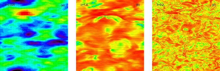
Figure 1. Contour map of intensity (color contour) and polarization vectors (black lines) projected along the LOS at different wavelengths. Left: at short wavelengths (λ = 0.02 in code units), Faraday rotation is negligible. Middle: at long wavelengths (λ = 1.4 in code units), we can see the effect of fluctuations of Faraday rotation and synchrotron emission. Right: at very long wavelengths (λ = 3.2 in code units), we can observe a strong Faraday depolarization effect. The mean magnetic field is along the horizontal direction.
Download figure:
Standard image High-resolution image4. Anisotropy of Polarized Synchrotron Intensity
4.1. Power Spectrum and Spatial Correlation of Synchrotron Polarization
Using synthetic data, Lee et al. (2016) found that the spectrum of PI changes as wavelength increases due to the effects of Faraday rotation, which is proportional to λ2. In this paper, we use real MHD turbulence data and obtain the power spectrum of PI arising from fluctuations of synchrotron radiation and Faraday rotation at different wavelengths. Figure 2 shows the results for two different cases: the direction of mean magnetic field is either perpendicular (left panel of Figure 2) or parallel (right panel of Figure 2) to the LOS.

Figure 2. Spectra of polarized intensity arising from fluctuations of synchrotron radiation and Faraday rotation. Different curves correspond to different wavelengths. Left: observed spectra of polarization arising from a region, in which mean magnetic field direction is along the y-direction. Right: polarization spectra from a region, in which the mean magnetic field direction is along the LOS.
Download figure:
Standard image High-resolution imageIn the left panel of Figure 2, we can see that, when the depolarization is insignificant, the spectrum goes up as the wavelength increases (λ = 0.02–1.4). This behavior of the power spectrum can be explained as follows. Since we have a strong mean magnetic field in the direction perpendicular to the LOS, the intrinsic synchrotron emission is more or less uniformly polarized. If we include Faraday rotation, it makes the polarization pattern deviate from the intrinsic state, which produces more fluctuations in polarization. Therefore, the spectrum goes up as wavelength increases. When the wavelength further increases, the depolarization effect affects large scales (i.e., at small-K's) more predominantly. As a result, the small-K part of the spectrum goes down, while the large-K part of the spectrum continues to move up, which is not affected by depolarization. Increase of the large-K part of spectrum implies that the Faraday rotation effect is more dominant than fluctuation of synchrotron polarization itself.
For the case of strong mean magnetic field along the LOS, the behavior of spectrum with different wavelengths is shown in the right panel of Figure 2. The spectrum at small-K goes down as wavelength increases unlike the spectrum for the mean field perpendicular to the LOS. Due to strong mean field along the LOS, which induces large Faraday rotation, polarization will be randomized at large scales (small-Ks) even at small wavelengths. However, we can still see the rise of spectrum at large-K (i.e., more fluctuations at small scales) for large wavelengths.
4.2. The Anisotropy of Synchrotron Polarization
In the presence of a strong mean magnetic field, turbulence structures become elongated along the mean field direction. In this section, we focus on how to describe this anisotropic structure. The structure function can be used to study statistics of synchrotron polarization in addition to the spectrum. In particular, the structure function for PI is useful to study the degree of anisotropy from a map. To visualize anisotropic structure, we first utilize the two-dimensional second-order structure function of PI

where r∥ is distance along the mean magnetic field and r⊥ is distance perpendicular to it. Since the mean magnetic field is along the x-direction, r∥ and r⊥ are increments in x- and y-directions, respectively.
We plot the structure functions for PI on the r∥ and r⊥ plane in Figure 3. The wavelengths for the panels are 0.02, 1.4, and 3.2 (left, middle, and right panels in Figure 3, respectively). In the left panel of Figure 3, we can clearly see that the structure is elongated along the mean field direction both on small scales and large scales. When Faraday depolarization effect begins to contribute, the structures on large scales start to lose their correlation (middle panel of Figure 3). As wavelength further increases, Faraday depolarization affects even smaller scales (right panel of Figure 3).
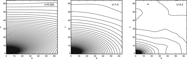
Figure 3. Contour map of polarized intensity (PI) at different wavelengths: λ = 0.02 (left), 1.4 (middle), and 3.2 (right) in code units.
Download figure:
Standard image High-resolution imageWe provide two types of complementary statistics to describe quantitatively the observed degree of anisotropy for PI. First, we plot the relation between  and
and  (left panel of Figure 4). The left panel of Figure 4 shows that all five curves representing five different wavelengths are below the red straight line, which denotes isotropic structures. The fact that all curves are below the red straight line implies that the structures are elongated along the mean field direction.5

Figure 4. Quantification of anisotropy of eddy shape. Left: ratio of y and x intercepts of the contours in Figure 3, which is equal to the ratio of perpendicular and parallel size of eddies. Red solid line represents isotropic structure. Right: quadrupole moments at different wavelengths drawn in different colors.
Download figure:
Standard image High-resolution imageSecond, we also calculate another statistic called QM, which is defined by

where ϕ is the polar angle subtended by the horizontal axis and a line connecting the points on the plane of the sky. The QM is zero for isotropic structures and the absolute value of it gets larger as anisotropy increases. If anisotropic structure is elongated along the direction of the horizontal axis (here, x-axis), the moment has negative values. For the opposite case, it has positive values.
The right panel of Figure 4 is the resulting QM. From the panel, we find that the moment remains unchanged when the wavelength is so small that the depolarization effect is negligible. As wavelength increases, Faraday depolarization becomes effective on large scales, and the absolute value of the moment goes down and approaches zero on large scales first. The absolute value of moment continues to decrease and approaches zero on smaller scales at longer wavelengths. Even at very long wavelengths, we can see anisotropy at small scales.
5. Polarized Synchrotron Emission from Two Spatially Separated Regions
In previous sections, we have considered a single volume, in which synchrotron emission and Faraday rotation happen simultaneously. In this section, we consider two synchrotron-emitting regions separated in space. That is, we suppose that polarized radiation comes from a turbulent background plasma (region 2 in Figure 5) and passes through another turbulent magnetized foreground medium (region 1 in Figure 5). Both regions have strong mean magnetic fields in directions perpendicular to the LOS. For simplicity, we assume that the mean magnetic fields are mutually perpendicular. The mean field in the background region is along the x direction, and that of the foreground region is along the y direction (see Figure 5). We assume that the average synchrotron intensities from the foreground and the background regions are either similar (Section 5.1) or different (Section 5.2).

Figure 5. Polarized synchrotron emission from two spatially separated regions. Polarized synchrotron emission arising from the background region (region 2), where the mean field is along the x direction, passes through the foreground region (region 1), where the mean field is along the y direction. The strength of the mean fields in both regions is the same. Red arrows indicate the directions of the mean fields.
Download figure:
Standard image High-resolution image5.1. Two Regions with Similar Synchrotron Emissivities
In the left panel of Figure 6, we plot the second-order structure function of observed polarized synchrotron intensity. In the figure, we also plot those from the foreground region (middle panel of Figure 6) and the background region (right panel of Figure 6) only. The structure functions in Figure 6 are plotted for a short wavelength in order to ignore the depolarization effect. The structures in regions 1 and 2 are elongated with respect to their own mean field directions. The observed structures in the left panel are isotropic because the observed emission is a mixture of the background emission, whose structure is elongated along the x direction, and the foreground emission, whose structure is elongated along the y direction.

Figure 6. Structure functions of polarized synchrotron emission from two spatially separated regions (see the cartoon in Figure 5). The left panel shows the structure function of the combined polarized synchrotron intensity from both regions. The middle and right panels show those from the foreground and the background regions, respectively.
Download figure:
Standard image High-resolution imageWe also visualize how the observed anisotropy of PI changes with wavelengths in Figure 7. At short wavelengths, we observe isotropic combined radiation emitted from both regions (left plot of Figure 7; the same as the left panel of Figure 6). However, when we observe it at longer wavelengths, we obtain anisotropic structures reflecting more dominantly those of the foreground region. This is because polarization arising from the background is negligible at longer wavelengths due to Faraday depolarization and, therefore, radiation from the region close to the observer contributes more to polarization structures. The middle and right panels of Figure 7 show structure functions at long wavelengths (λ = 1.4 and 3.2). As the wavelength increases from 1.4 to 3.2, the correlation on large scales gets gradually weaker and anisotropy is observed on progressively smaller scales. In both panels, the anisotropy on small scales is along the mean field direction of the foreground region. The very weak correlation on large scales at λ = 3.2 is due to enhanced Faraday rotation.
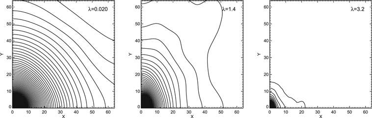
Figure 7. Contour map of observed polarized intensity at different wavelengths: λ = 0.02 (left), 1.4 (middle), and 3.2 (right) in code units.
Download figure:
Standard image High-resolution imageAs wavelength increases, observed anisotropy begins to reflect that of the foreground region. As a result, the behavior of the moment more or less resembles that of the single emitting region (see the middle panel of Figure 8). That is, the moment is a decreasing function of separation r and it is close to zero when r is larger than a certain value. As wavelength increases, the moment declines faster.

Figure 8. Quadrupole moment of polarized synchrotron intensity from two spatially separated regions. The left panel shows the moments of the combined emission from both regions. The middle and right panels show those from the foreground and the background regions, respectively. Faraday rotation in the foreground region is included in the calculation of the quadrupole moments in the right panel.
Download figure:
Standard image High-resolution imageFrom left to right in Figure 8, we plot the QM of PI from combined regions, the foreground region only, and the background region only. Note that, for the case of the background region only, the foreground region also contributes to Faraday rotation of the background emission. In the left panel of Figure 8, when the wavelength is very short (λ = 0.02; black solid curve), the intrinsic emissions are not affected by Faraday rotation and their structures are nearly isotropic due to the averaging effect at all scales. Therefore, the moment is almost zero on all scales. For λ = 0.56 (blue dotted line), emissions from both foreground and background regions are depolarized and become isotropic at the largest scales. However, only emission from the background region is depolarized in intermediate scales near R = 50 (see the middle and right panels of Figure 8). Therefore, the QM is positive due to anisotropic structure in the foreground region. At very small scales, emissions from both foreground and background regions are not strongly affected by Faraday depolarization and, hence, combined polarized emissions from foreground and background regions become isotropic due to the average effect. The resulting QM is nearly zero at very small scales (see the cyan curve in Figure 8). At a longer wavelength (e.g., λ ∼ 1.4), the emission from the background region is depolarized at all scales (see the right panel of Figure 8) and emission from the foreground region is depolarized at large scales (e.g., R > 50 for λ ∼ 1.4). As a result, the QM has large positive values at small scales and has nearly zero value at large scales (see the green curve in the left panel of Figure 8). In other words, we can see the anisotropy of polarized emission from the foreground region at small scales if we observe at a long wavelength.
5.2. Two Regions with Different Synchrotron Emissivities
A number of observations imply such a situation that synchrotron radiation mainly originates in the Galactic halo while the effect of Faraday rotation is stronger in the Galactic disk. The latter is supported by the fact that the r.m.s. fluctuation of Galactic rotation measure peaks strongly at the Galactic midplane (Taylor et al. 2009). Therefore, in this subsection, we consider three cases:
- 1.Case 1. Both foreground and background produce similar amounts of Faraday rotation, but the background has stronger synchrotron emissivity.
- 2.Case 2. Both regions have similar synchrotron emissivities, but the foreground produces stronger Faraday rotation.
- 3.Case 3. The background has stronger synchrotron emissivity and the foreground produces stronger Faraday rotation.
Our main concern is Case 3. However, we also consider Case 1 and Case 2 for the sake of completeness.
Let us consider Case 3 first, in which we assume that the emission from the background region is five times stronger than that from the foreground region and the RM in the foreground region is five times larger than that in the background region. With these assumptions, we calculate structure function and its QM. Figure 9 is the structure function of the observed PI. At short wavelengths, Faraday rotation is negligible and anisotropic structure samples that of the stronger emission, which is the background emission in our case (left panel of Figure 9). As wavelength increases (λ ≳ 1.4), emission from the background goes through more Faraday depolarization than that from the foreground and therefore the observed structure is similar to that of the foreground. At very long wavelengths (λ ∼ 3.2), we can see that most structures are uncorrelated or weakly correlated and only small-scale structures maintain its anisotropy (Figure 9(c)). In fact, anisotropic structures are correlated when  , where l is the size of the foreground and
  is magnetic field parallel to the LOS.6
We can obtain information on the magnetic field direction of foreground region from observed structure function below the scale. Note that the anisotropic structure on large scales
is magnetic field parallel to the LOS.6
We can obtain information on the magnetic field direction of foreground region from observed structure function below the scale. Note that the anisotropic structure on large scales  in Figure 9(c) could be a numerical artifact. We can see artificial anisotropic structure on large scales caused by discrete Faraday sources along the LOS when we observe polarization structure at very long wavelengths (see A.3 of Lazarian & Yuen 2018b).

Figure 9. Structure functions of polarized synchrotron emission from two spatially separated regions with different synchrotron emissivities and Faraday rotation. From left to right panels, the observed wavelength increases: λ = 0.02 (left), 1.4 (middle), and 3.2 (right). We assume (1) thermal electron number density responsible for Faraday rotation in the foreground is 5× larger than that in the background, and (2) synchrotron radiation in the background is 5× stronger than that in the foreground. The thermal electron density in the foreground and synchrotron radiation in the background are the same as the ones in our earlier calculations (see, for example, Section 5.1).
Download figure:
Standard image High-resolution imageTo quantify anisotropic structures of polarized synchrotron emission from two regions, we calculate QM for three different cases mentioned above. We plot the QM for Case 1 in the left panel of Figure 10. At short wavelengths (λ < 1.4: black and blue lines), since Faraday rotation has no impact on the structure of polarized radiation, we see negative QM reflecting anisotropy of the background region where synchrotron emission is stronger. However, at a long wavelength (λ = 1.4: green dashed line), emission from the background is depolarized and the observed structure is indicative of QM in the foreground, which is positive. When wavelength is very long ((λ = 3.2: red dotted–dashed line), we see anisotropy (i.e., positive QM) only on very small scales. We also plot QM for Case 2 in the middle panel of Figure 10. At short wavelengths, QM is nearly zero. This is because, since both the foreground and background have similar synchrotron emissivities, the combined emission from them is virtually isotropic. As wavelength increases (λ ≳ 1.4), strong rotation measure of the foreground region attributes to fast depolarization of background emission and hence the observed QM reflects more predominantly that of the foreground. Therefore, compared with those for Case 1, the QMs for Case 2 have larger positive values. The right panel of Figure 10 shows the QM for Case 3. At short wavelengths, the QM mainly reveals that of the background region due to strong synchrotron emission from the background. At longer wavelengths (λ ≳ 1.4), QM has high positive values, representing elongated structure along the y-direction, within the scale,  . We also see negative values because of artificial anisotropic structure elongated along the x-direction at very long wavelengths (λ ∼ 3.2).

Figure 10. Quadrupole moment of polarized synchrotron intensity from two spatially separated regions with different synchrotron emissivities and Faraday rotation. Quadrupole moments in all panels are based on the combined emissions from both regions. Each panel shows the moments for three different cases. Left: the synchrotron emissivity in the background is 5× larger than that in the foreground (Case 1). Middle: the amount of Faraday rotation in the foreground is 5× larger than that in the background (Case 2). Right: the amount of Faraday rotation in the foreground is 5× larger than that in the background, and synchrotron radiation in the background is 5× stronger than that in the foreground, which corresponds to the case in Figure 9 (Case 3). Note that nonenhanced quantities are the same as those in our earlier calculations (see, for example, Section 5.1).
Download figure:
Standard image High-resolution image6. Discussion
6.1. Comparison with Other Ways of Probing Magnetic Field with Polarized Synchrotron
As we mentioned earlier, the measurement of polarized synchrotron radiation is not a reliable way to probe the plane of the sky magnetic field structure from a volume that both emits synchrotron radiation and is subject to appreciable Faraday rotation. Using high frequencies at which Faraday rotation is negligible, one can obtain the 2D structure of magnetic field projected on the plane of the sky. The same information can also be obtained with Synchrotron Intensity Gradients (SIGs; Lazarian et al. 2017) for any frequency of measurements as the intensities are not subject to Faraday rotation.
Faraday tomography based on the approach proposed by Burn (1966) allows us to get insight into 3D distribution of the LOS component of magnetic field. The technique has its own problems for studying turbulent magnetic fields, however (see Lazarian & Yuen 2018b). Nevertheless, it can be considered as complimentary to what we suggested in this paper.
The closest in spirit technique is the SPG technique proposed in Lazarian & Yuen (2018b). The relation between our approach and that of the SPG is similar to the relation between the Correlation Function Anisotropy technique (Lazarian et al. 2002; Esquivel & Lazarian 2005, 2011) and the velocity gradients (see Yuen & Lazarian 2017; Lazarian & Yuen 2018a). The latter two techniques were compared in Yuen et al. (2018). The advantage of gradients is that they provide a more detailed structure of magnetic field. The advantage of studying anisotropy of correlation functions is that a more detailed analysis of the contribution of compressible and Alfvénic modes is possible. For the case of synchrotron emission this is possible due to the analytical description of the synchrotron statistics in Lazarian & Pogosyan (2012, 2016). We plan to perform the corresponding study elsewhere.
6.2. Essence of the Technique
In this paper, we described observed anisotropic structure of polarized synchrotron intensity using second-order structure function and QM. In particular, second-order structure function visualizes anisotropic structure of PI and the QM quantifies the degree of its anisotropic structure. It is evident that the former can trace the direction of the mean magnetic field from the elongation of its contour map if there is no Faraday rotation.
The structure function can be used to identify the direction of the mean magnetic field even in the presence of Faraday rotation. Figure 1 shows how the polarization map changes as wavelength increases. At short wavelengths where the Faraday rotation effect is negligible, its structure is elongated along the horizontal direction, which is the direction of the mean magnetic field. The direction of polarization rotated by 90 degrees are also aligned with the direction of the mean magnetic field (left panel of Figure 1). At longer wavelengths where Faraday rotation is significant, depolarization makes polarization directions randomized, which results in large-scale structures more or less isotropic. Note, however, that the structures at small scales are still elongated along the mean field direction (middle and right panels of Figure 1). Therefore, we can reveal correct anisotropy, and the direction of the mean magnetic field, at small scales if we use the second-order structure function. In summary, Faraday rotation depending on observation wavelength affects large-scale structures first and we see uncorrelated large-scale structures with disordered direction of polarization at long wavelengths. Even though large-scale structures fail to present ordered shapes, the second-order structure function of the PI still indicates the direction of mean magnetic field at small scales when observation is performed at a long wavelength where Faraday rotation effect is too important to be ignored.
Comparison of QM with power spectrum enables us to help clarify the process of depolarization by Faraday rotation as wavelength increases. As we can see in the left panel of Figure 2, the spectrum goes up without changing its shape much as wavelength increases when wavelength is small (see black and blue curves). During this process, QM does not exhibit notable change (see black and blue curves in the right panel of Figure 4). However, as wavelength further increases, the spectrum and the quadrupole behave differently: the spectrum continuously goes up, but the QM deviates from those for small wavelengths (see green curves for λ ∼ 0.9). This result may imply that Faraday depolarization at its early stage does affect anisotropic structures, although it does not influence the magnitude of PI much. When λ ∼ 1.4, large-scale power becomes suppressed by Faraday depolarization and, as a result, the spectrum at small-K's stops increasing, while that at large-K's continues to go up (see the curve for λ ∼ 1.4). A detailed explanation for this spectral behavior can be found in Lee et al. (2016). By comparison, as depolarization begins, the QM decreases and goes to zero at large scales first (see the curve for λ ∼ 1.4 in the right panel of Figure 4), which means that depolarization destroys anisotropic structures.
6.3. Studies of Disk and Halo Magnetic Fields
The structure of polarization by synchrotron emission and Faraday rotation can be used to obtain properties of magnetic field in Galactic disk and halo. Observations of Faraday rotation measure have been carried out and found the dependence of rotation measure on the Galactic latitude: the RMs close to the Galactic plane are much larger than RMs at high Galactic latitudes (National Radio Astronomy Observatory VLS Sky Survey; Taylor et al. 2009). In fact, the amplitude of large-scale RM structures near the Galactic plane is ∼100  and its amplitude for high latitudes is ∼20
  (Taylor et al. 2009; Schnitzeler 2010). If we adopt the free electron distribution model of Gaensler et al. (2008), the RM arising from the Galactic disk dominates that from the halo when Galactic latitude is roughly less than 30° (Taylor et al. 2009). However, when it comes to synchrotron emission, it is likely that emission from the Galactic halo is stronger. To model this, we have assumed the rotation measure in the Galactic disk is five times larger than that in the Galactic halo and synchrotron radiation and Faraday rotation occupy separate volumes in Section 5.2. Here, we assume that we are observing toward a low Galactic latitude (e.g., b ∼ 10°). In this case, the RM arising from the Galactic disk for the LOS is around 70
  , if we assume ne = 0.01 cm−3 (Gaensler et al. 2008 see also Cordes & Lazio 2004; Nota & Katgert 2010),
  , and L ∼ 7 kpc, where L is the path length. In the simulation, the RM of the foreground is ∼7.5 in code units. In our simulation, anisotropy of polarization map samples the direction of mean magnetic field in the background at λ ≲ 0.6, and it reflects the direction of mean magnetic field in the foreground at λ ≳ 1.4 in code units. If we convert λ = 1.4 in code units to real units, it corresponds to λ ∼ 45 cm. Therefore, we expect to study the direction of mean magnetic field in the background (i.e., Galactic halo) when λ ≲ 20 cm. It is likely that anisotropy reflects the direction of mean magnetic field in the foreground (i.e., Galactic disk) if λ ≳ 45 cm.
6.4. Applicability of Adiabatic Condition for Faraday Rotation
In this paper, we have assumed that a linearly polarized electromagnetic wave in a plasma can be decomposed into two independent eigenmodes, left and right circularly polarized waves. As they propagate independently (or, adiabatically) in a magnetized plasma, they produce Faraday rotation as given in Equation (3).
However, Broderick & Blandford (2010) showed that, at sufficiently low frequencies, "the character of Faraday rotation changes, entering what they term the super-adiabatic regime in which the rotation measure (RM) is proportional to the integrated absolute value of the LOS component of the field." That is, at very low frequencies, the left and the right circularly polarized waves become no longer independent and, hence, we cannot use Equation (3) anymore.
The critical frequency for the super-adiabatic regime is
where lB is the local magnetic field reversal length scale and νSA typically ranges from 10 kHz to 10 GHz (Broderick & Blandford 2010). For Galactic halo, we expect that the critical frequency is νSA ∼ 15 kHz, which corresponds to λSA ∼ 2 × 106 cm. Here, we use n ∼ 0.003 cm−3, B ∼ 1 μG, and lB = 100 pc, which could be the outer scale of turbulence in the Galactic halo. This critical wavelength is much longer than the wavelengths discussed in the previous subsection. Therefore, it may not be necessary to consider the effects of nonadiabatic propagation for Faraday rotation in the Galactic halo.
7. Summary
We have studied the structure of PI using statistics such as power spectrum, structure function, and QM. This study demonstrates that it is possible to reconstruct the structure of magnetic field using observed fluctuations of polarized synchrotron radiation.
- 1.Using structure function, we visualize how the structures are elongated and QM can measure the degree of elongation (anisotropy). Structure function and QM show that depolarization happens in large scales first and anisotropic structures at small scales are still existent at longer wavelengths.
- 2.Polarized intensity map gives information about the direction of mean magnetic field since PI maintain the direction of anisotropic structure even at long wavelengths, whereas directions of polarization are randomized at short wavelengths due to Faraday rotation.
- 3.If there are two synchrotron-emitting volumes, the observed polarization reflects the anisotropy of PI coming from the foreground region at long wavelengths.
- 4.If there are two synchrotron-emitting volumes with different emissivity, anisotropy changes its direction with wavelengths: at short wavelengths, the map shows the structure of the background region, and at long wavelengths shows the structure of the foreground region.
This paper has been expanded from a chapter of Hyeseung Lee's Ph. D. thesis. H.L. and J.C.'s work is supported by the National R&D Program through the National Research Foundation of Korea Grants funded by the Korean Government (NRF-2016R1A5A1013277 and NRF-2016R1D1A1B02015014). A.L. acknowledges the NSF AST 1816234.
Footnotes
- 4
We put "isotropic" in quotes, as it is explained in LP12 that the isotropy is related to the functional part, but not the tensor form of the expression that describes the fast mode correlations.
- 5
If the model of Goldreich & Sridhar (1995) is correct, we expect
 and in the inertial range. Therefore, we expect to see a power-law relation between the horizontal and the vertical axes. However, we do not see a power-law relation because the contours are calculated in the global frame.
 - 6
This is true when there are less than a few independent eddies along the LOS.

