


Abstract
We investigate the dependence of solar, plasma, and geomagnetic parameters' periodicities on the heliospheric magnetic field polarities for the past five solar activity cycles (1967–2016). For this purpose, the Morlet wavelet technique has been performed to extract information about significant periods. The monthly averages of toward ( ) and away (
 ) polarity groups have been calculated for each parameter. The solar and plasma parameters used in this work are the interplanetary magnetic field (
 ), sunspot numbers (
 ), and solar plasma speed (
 ), and the geomagnetic indices
  ,
,  , and
, and  . We found that the wavelet power spectra (WPS) for the monthly averages of
  and
and  nearly showed a symmetrical power spectra distribution. The global wavelet spectra (GWS) for
  and
and  displayed a coupling at some level between 3.2–3.5, 10.7, and 18.3 yr of variations. The GWS for
  provided two significant peaks, within the 95% confidence level, at 9.8 and 15.2 yr, as well as at 1 and 9.8 yr, for
  . In addition, the existence of a periodicity of 1 yr is obvious for
  spectra and it shifted to a 1.5 yr variation in
  spectra. Both the WPS and GWS for
  and
and  reflect symmetric power spectra for both groups in the northern and southern hemispheres. The
  spectra exhibited prominent periodicities at 10.7 yr for
  and 9.8 yr for
  . Also, the well-known 9.8 yr periodicity variation is a dominant variation in both the spectra of
  and
and  . On the other hand, within the cone of influence, the periodicities of 10.7 and 13.9 yr are observed for the
  spectra and 9.8 yr for
  spectra. The GWS showed double-peak structure for the spectrum of
  .
.
Export citation and abstract BibTeX RIS
1. Introduction
1.1. Features of the Solar Magnetic Field and the Heliosphere
The solar and space science community specialists believe that the heliospheric magnetic field (HMF), which is a component of the Sun's magnetic field, is dragged out by the solar wind (SW) from the solar corona to the interplanetary medium. The northern and southern solar hemispheres have opposite polarities of HMF. Along the plane of the Sun's magnetic equator, the magnetic field lines run anti-parallel to each other and are separated by a thin neutral current sheet known as the heliospheric current sheet (HCS). The HCS is believed to have a wavy structured form (HCS tilts) as it extends into interplanetary medium. Around the times of solar activity maxima, the polarities of the solar polar magnetic field and the heliosphere reverse their directions systematically. During a positive magnetic polarity epoch (qA > 0), such as during periods 1971–79 and 1991–99, the magnetic field emerged from the Sun in the northern hemisphere and was directed toward the Sun in the southern hemisphere. The opposite configuration (when the HMF is directed toward the Sun in the northern hemisphere and away from the Sun in the southern hemisphere), as in the periods 1981–89 and 2001–12, is referred to as the negative magnetic polarity epoch (qA < 0). These polarities are opposite in opposing hemispheres, as well as from one solar cycle to the next (this is known as Hale's cycle, which lasts ∼22 yr). The polar fields are thus in anti-phase with the sunspot cycle as the polar magnetic field maximizes near the times of solar activity minima. Since 1970 June, the polarity of the solar polar magnetic field near 1 au has been measured almost daily by the Wilcox Solar Observatory (WSO) at Stanford University. The irregularity of solar activity phenomena (such as; HMF, sunspot numbers (SNs), sunspot areas (SAs), 10.7 cm solar radio flux (SF), etc.) between northern and southern solar hemispheres is referred to as the north–south (N–S) asymmetry. The N–S asymmetries of solar and plasma parameters have been studied by several authors (e.g., El-Borie 2001; El-Borie et al. 2012 and references therein). Recently, based on the asymmetry between the solar polar field north and south of the HCS, toward or away from the Sun, El-Borie et al. (2016) studied the N–S asymmetry of the HMF magnitude and geomagnetic indices (aa, Kp, Ap, and Dst) over the period 1975–2013. The study showed that there was an absence of N–S asymmetry of the HMF magnitude over the grand average of each solar cycle (20th–23rd). In addition, the geomagnetic indices exhibited a noticeable asymmetry during the positive solar magnetic polarity epoch (qA > 0), and they had a northern dominance during some solar cycles (22 and 23), while the asymmetry shifted to southern dominance during other solar cycles (21 and 24). More recently, El-Borie et al. (2018a) studied the asymmetries in the HMF magnitude and SW plasma properties as functions of the HMF polarity (toward or away). The study presented similar analyses for solar indices (SNs and SF), as well as the dependence of the asymmetries on solar activity cycle. The period extended from 1967 to 2016 (throughout the last five solar activity cycles, 20th–24th). The results showed that, for the toward polarity group, the yearly average of solar plasma velocity was faster than the yearly average of solar plasma velocity for the away polarity group by 13 km s−1 and 16 km s−1 during solar cycles 21 and 23, respectively. In contrast, the yearly average of solar plasma velocity for the away polarity group was greater than the yearly average of solar plasma velocity for the toward polarity group by about 17.5 km s−1 during solar activity cycle 23. Additionally, the solar plasma was hotter during the toward than the away polarity days during solar cycles 21, 22, and 24, while it was cooler during the toward than the away polarity days during solar activity cycles 20 and 23. The solar disk exhibited uniform activity for both toward and away polarity groups during solar cycles 20 and 23. In contrast, the solar activity was greater in the toward polarity group than the away polarity group during solar cycle 22. On the other hand, during solar cycles 21 and 24, the solar activity shifted to away polarity days. Moreover, the solar parameters exhibited a non-uniform distribution. In addition, the impact of the asymmetrical distribution of solar activity features on HMF magnitude, plasma, and solar parameters recorded nearby Earth at 1 au over a period of 50 yr has been studied (El-Borie et al. 2018b). The data were sorted into to two groups (northern and southern) according to the dominance of SAs in the northern or southern solar hemisphere. The study showed that during the past five solar activity cycles (20–24), the average differences of HMF magnitude for both the northern and southern groups were statistically insignificant. Moreover, the solar plasma from the sorted northern group was faster than that of the southern activity group by 6.16 ± 0.65 km s−1, 5.70 ± 0.86 km s−1 and 5.76 ±1.35 km s−1 during 1972, 2002 and 2008, respectively. On the other hand, the yearly average of solar plasma temperature for the northern solar activity group was greater than that of the southern group for 17 yr out of 50 yr. The asymmetries showed that the northern group highly predominated the southern one in different two years (1972 and 1996), while two significant equivalent southern peaks occurred in 1978 and 1993. In addition, the grand average of the SN showed symmetric activity for the northern and southern groups throughout solar cycles 20 and 21. In contrast, the solar activity represented by sunspots tended to have southern dominance during solar cycles 22 and 23, while the activity shifted again to a symmetric distribution on both solar hemispheres during solar cycle 24. El-Borie et al. (2018c) studied the N–S asymmetry of geomagnetic indices (aa, Ap, Kp, and Dst) based on the HMF polarity (toward or away). The results showed that the geomagnetic indices exhibited considerable N–S asymmetry throughout the entire period (1967–2016). Regarding the aa, Ap, and Kp geomagnetic indicies, the positive magnetic polarity epoch (1971–1979) showed geomagnetically northern dominance, while the negative magnetic polarity epoch (2001–2012) showed southern geomagnetic dominance.
1.2. The Wavelet Power Spectra
Extracting the periodicities in a time series can be determined by different tools such as the fast Fourier transform, the maximum entropy method, and the Morlet wavelet transform technique. The Fourier transform is a useful tool for analyzing the frequency components of time series. However, the weakness of a fast Fourier transform is that if we take fast Fourier transforms over the full time series, we cannot tell at what moment a specific frequency or period rises. To find the spectrogram, a short-time Fourier transform uses a sliding Hanning window: this provides information on both time and frequency. Another problem persists, however: the length of the window limits the resolution in frequency. Astronomical synthesis commonly employs the maximum entropy method, which is commonly employed in imaging. In this application, the signal-to-noise ratio determines the resolution, which must be specified. Resolution is thus image-dependent and varies across the map. This means that the maximum entropy method is also biased, for the ensemble average of the estimated noise is nonzero. However, the noise for pixels is much more than that for bias. The bias detected can yield a super-resolution, which can usually be trusted to an order of magnitude in solid angle. The Morlet wavelet technique is a better way compared to other period investigation techniques. It permits evaluating possible temporal variations of the oscillations detected in a time series. This technique has additionally been broadly utilized as a part of solar physics. The Morlet wavelet technique maps a one-dimensional signal onto a timescale plane and allows the time history of the spectral signal properties to be analyzed. It is additionally an efficient way for determining hidden periodicities in time series. Unlike the Fourier transform, the wavelet transform allows not only characteristic scales (frequencies) of periodicities to be determined but also their localization on the time axis to be detected (Ippolitov et al. 2002). However, the discrete wavelet transform of a signal  can be written in the following form:
where Wk(s) are the wavelet transform coefficients, s is the scale, k is the shift along the time axis, δt is the time period between the adjacent measurements, and ψ is the wavelet function. Instead of Equation (1), the equivalent expression can be written as follows:
where ![${\widehat{{\rm{\Psi }}}}^{* }\left(s{\omega }_{n}\right)={\left[\tfrac{2\pi s}{\delta t}\right]}^{1/2}.{\widehat{{\rm{\Psi }}}}_{o}\left(s{\omega }_{n}\right)$](https://content.cld.iop.org/journals/0004-637X/880/2/86/revision1/apjab12d8ieqn28.gif) and
and  , whereas N is the number of points in the time series, and ψo is the basic wavelet function for which we took the Morley wavelet that localized in the time and frequency domains. Here, t is a dimensionless parameter:
Singh & Badruddin (2014) implanted the wavelet analysis on daily, monthly, and yearly time series of solar and geomagnetic parameters in order to study the periodicities in these parameters in search of the relation between solar variability and variations in other phenomena. Their results indicated there were periodicities of 27.8, 157, 370 days, and 2.2, 5.5, 11, 22.7, 38.6 yr in the SN, as well as 13.8, 26.6, 185 days, and 5.3, 11, 30, 46 yr in the geomagnetic aa index. The 11 yr periodicity was the most significant periodicity in SN as well as in aa-index data using the daily, monthly, and yearly data, which is consistent with earlier studies. It was also suggested that at least periodicities in geomagnetism, which were composed of 27 days, 5.3, and 11 yr in both SN and aa-index data, have a solar origin. In addition, the same analysis of power spectra has been implemented on daily data of the solar activity indicators (SN and SF), geomagnetic activity (Ap index), and cosmic-ray intensity (neutron monitor count rate) to study the short-term and mid-term oscillations of these parameters during two solar magnetic cycles (1968–1989 and 1989–2014) by Singh & Badruddin (2017). The results showed that significant power density, in addition to fundamental periods, like 27 days (solar rotation period), 154 days (Rieger period), semi-annual, annual, 1.3, and 1.7 yr, were also observed with a few quasi-continuous and noncontinuous oscillations. In the geomagnetic Ap index during both the magnetic cycles, the solar rotation (∼27 days), the second harmonic (13.5 days) and third harmonic (9 days) were observed. Furthermore, the annual and ∼1.85 yr variations are also observed in all the considered parameters with good signatures in cosmic-ray intensity. In 2014, Jayalekshmi & Prince studied the periodicities in the sunspots Rz (1749–2010) and Dst geomagnetic index (1957–2010). Peaks at 10.7 and 110.7 yr were found as the significant periodicities for Rz during the period (1749–2010). Moreover, during the period 1916–2010, it was found that the most prominent periodicity was 9.8 yr. The dominant periodicity in Dst index during the years 1957–2010 was 10.7 yr. Besides the periodicity at 10.7 yr, other periodicities such as 11.6, 9.8, and 12.7 yr were significant around the years 1964 and 2002. On the other hand, Wei et al. (2004) studied the power-law dependence of the geomagnetic Dst index using wavelet transforms. The results showed that the Dst index possesses properties associated with self-affine fractals similar to the power spectral density and obeys a power-law dependence on frequency. In fact, the behavior of the Dst index, with a Hurst exponent H ≈ 0.5 (power-law exponent β ≈ 2) at high frequency, is similar to that of Brownian motion. They suggested that the dynamical invariants of the Dst index might be described by a possible Brownian motion model. Statistically significant intermediate-term periodicities of the N–S asymmetry of SA data have been investigated using Lomb–Scargle and wavelet techniques (Chowdhury et al. 2013). The study showed that several short-term and mid-term periods including the best-known Rieger one (150–160 days) are detected in cycle 23 and near Rieger-type periods during cycle 24, and most of them are found to be time-variable.
In the present study we perform the wavelet power spectra technique to study the dependence of solar, plasma, and geomagnetic parameters' oscillations on the HMF polarities and compare the obtained results for solar, plasma, and geomagnetic indices during the time interval 1967–2016. The presented analysis was quite extensive and is of interest to the heliospheric community. On the basis of the observational results and discussions, we have summarized the important conclusions.
2. Data and Analysis
It is known that based on hourly averages, the daily HMF direction can be determined by using the geocentric solar ecliptic (GSE) coordinates. Thus, the direction of the HMF is separated into two polarities: when the solar ecliptic azimuthal angle of the HMF daily average lies between 225° and 360° and between 0° and 45° the direction is referred to as toward ( ) polarity and otherwise it is referred to as away (
 ) polarity. In the present work, we used only the well-defined HMF days over the period from 1967 to 2016. Days of mixed HMF polarities or missing data were removed from our analysis. We sorted the data into two groups; toward and away HMF polarity days. The daily means of HMF direction were taken via
  https://omniweb.gsfc.nasa.gov/html/polarity/polarity_tab_html
 . In addition, the selected daily data of SNs (
 ), plasma velocity (
 ), and geomagnetic indices (
 ,
,  , and
, and  ) that were taken via
  http://omniweb.gsfc.nasa.gov/form/dx1.html
 have been sorted into two groups based on
  and
and  daily HMF directions. The monthly averages of the
  and
and  polarity groups have been calculated for each parameter.
  ,
,  ,
,  ,
,  ,
,  , and
, and  refer to the monthly averages of the toward polarity group for
  ,
,  ,
,  ,
,  ,
,  , and
, and  , respectively. On the other hand,
  ,
,  ,
,  ,
,  ,
,  , and
, and  refer to the monthly average values of the away polarity group for
  ,
,  ,
,  ,
,  ,
,  , and
, and  , respectively. The gaps were filled by cubic spline interpolation, and as a final procedure, the solar magnetic field
  , plasma velocity
  , SN
, SN  , and the geomagnetic
  ,
,  , and
, and  indices, have been analyzed using the wavelet analysis technique to extract information about significant periods. In the present work, we used the Morlet wavelet analysis (Torrence & Compo 1998) to study the mid- and long-term periodicities for the solar, plasma, and geomagnetic indices of the away and toward polarity groups, separately.
3. Results and Discussion
Figure 1 represents the scatter plots between the monthly averages of  and
and  (plot a),
  and
and  (plot b),
  and
and  (plot c), and
  and
and  (plot d). The correlation coefficient (r), which measures the strength and direction of the linear relationship between two variables on a scatter plot, and the regression line equation between the
  and
and  values of each parameters, are also shown. The scatter plots show that
  and
and  as well as
  and
and  exhibited good correlation between each of the two parameters. The correlation coefficients are 0.57 and 0.41, respectively. In addition, the scatter plot between
  and
and  shows a strong significant correlation (r = 0.9). In contrast, the scatter plot between
  and
and  shows the positive moderate correlation. Furthermore, the slope of the regression line, i.e., a measure of how the sensitivity of the
  value changes based on the change in
  value, is highly significant in the case of
  and
and  than it is for the other parameters. Table 1 shows the regression equations and the correlation coefficients between the monthly averages for the
  and
and  values for the selected parameters.
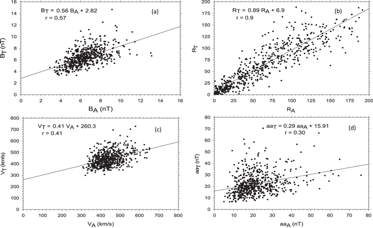
Figure 1. Scatter plots of monthly  and
and  values for
  (panel (a)),
  (panel (b)),
  (panel (c)), and
  (panel (d)). The regression equation and the correlation coefficient between the monthly
  and
and  values for each parameter are also shown.
Download figure:
Standard image High-resolution imageTable 1.
The Regression Relation between the Monthly Averages of  and
and  Values for
  ,
,  ,
,  ,
,  ,
,  , and
, and  Parameters from 1967 to 2016
| Parameter | Regression Relation between Monthly  and and  Values of Each Parameter Values of Each Parameter |
Correlation Coefficient (r) |
|---|---|---|
| IMF Magnitude (B) | BT = 0.56 BA+2.82 | 0.57 |
| Plasma Flow Speed (V) | VT = 0.41 VA+260.3 | 0.41 |
| Sunspot Numbers (R) | RT = 0.89 RT+6.9 | 0.90 |
| aa Index | aaT = 0.29 aaA+15.91 | 0.30 |
| Kp Index | KpT = 0.43 KpA+12.47 | 0.41 |
| Ap Index | ApT = 0.27 ApA+9.5 | 0.28 |
Note. The correlation coefficient (r) and the regression relation between monthly average and values of each parameter are also listed in the table.
Download table as: ASCIITypeset image
Figure 2 displays the time series of the relative amplitudes of the smoothed monthly of ![${B}_{T}/[{B}_{T}+{B}_{A}]$](https://content.cld.iop.org/journals/0004-637X/880/2/86/revision1/apjab12d8ieqn117.gif) (plot a),
(plot a), ![${R}_{T}/[{R}_{T}+{R}_{A}]$](https://content.cld.iop.org/journals/0004-637X/880/2/86/revision1/apjab12d8ieqn118.gif) (plot b),
(plot b), ![${V}_{T}/[{V}_{T}+{V}_{A}]$](https://content.cld.iop.org/journals/0004-637X/880/2/86/revision1/apjab12d8ieqn119.gif) (plot c), and
(plot c), and ![${{aa}}_{T}/[{{aa}}_{T}+{{aa}}_{A}]$](https://content.cld.iop.org/journals/0004-637X/880/2/86/revision1/apjab12d8ieqn120.gif) (plot d). The data were smoothed over 13 months using the running averages method. The figure shows clear oscillations of smoothed averaged monthly solar, plasma, and geomagnetic parameters in all investigated cycles. To reveal the details of these periodic variations, we plot in Figures 3–8 the periodograms of the temporal evolution of the wavelet power spectrum (WPS) and the GWS for the following parameters:
(plot d). The data were smoothed over 13 months using the running averages method. The figure shows clear oscillations of smoothed averaged monthly solar, plasma, and geomagnetic parameters in all investigated cycles. To reveal the details of these periodic variations, we plot in Figures 3–8 the periodograms of the temporal evolution of the wavelet power spectrum (WPS) and the GWS for the following parameters:  ,
,  ,
,  ,
,  -index,
  -index, and
  -index, respectively. Each figure has two plots (a and b) based on the interplanetary magnetic field sense, toward (
 ) or away (
 ), respectively. In the WPS, the y axis provides information about the periodicity in years, and the x axis gives the time observation of the data. Moreover, the levels of spectral power corresponding to each variation at different time periods can be clarified through the information on the contours. The thick (black line) contour represents the region of the spectrum of the 95% confidence level. In the GWS (right plot), the variation of power is shown with its period, and the thick dashed line is the 95% confidence level. The cone of influence (COI) is also shown in the wavelet spectra that describe the region influenced by the zero padding or show edge effect.
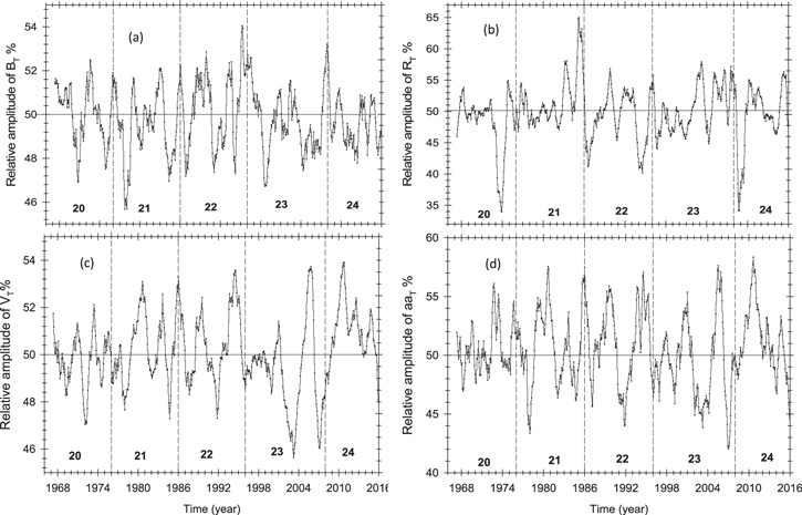
Figure 2. Relative amplitudes of smoothed monthly (a) BT/[BT+BA], (b) RT/[RT+RA], (c) VT/[VT+VA], and (d) aaT/[aaT+aaA] from 1967 to 2016. The data are smoothed over 13 months. The solar cycles are numbered on each plot. The vertical dashed lines represent the times of minima of the solar activity cycle.
Download figure:
Standard image High-resolution image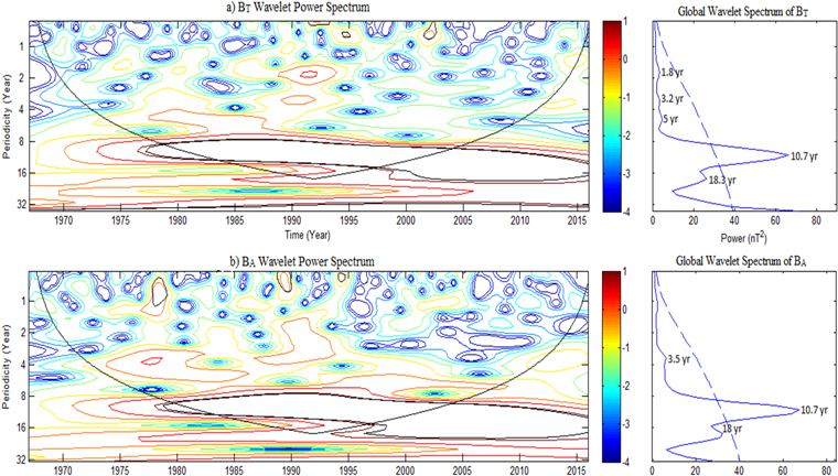
Figure 3. WPS and GWS of the field magnitude  , based on the HMF polarity, for the monthly averages of the toward (
 ; top plots) and away (
 ; bottom plots) sectors, over the period 1967–2016.
Download figure:
Standard image High-resolution image
Figure 4. WPS and GWS of the solar plasma velocity  , based on the HMF polarity for the monthly averages of the toward (
 ; top plots) and away (
 ; bottom plots) sectors, over the period 1967–2016.
Download figure:
Standard image High-resolution image
Figure 5. WPS and GWS of the sunspot number  , based on the HMF polarity, for the monthly averages of the toward (
 ; top plots) and away (
 ; bottom plots) sectors, over the period 1967–2016.
Download figure:
Standard image High-resolution image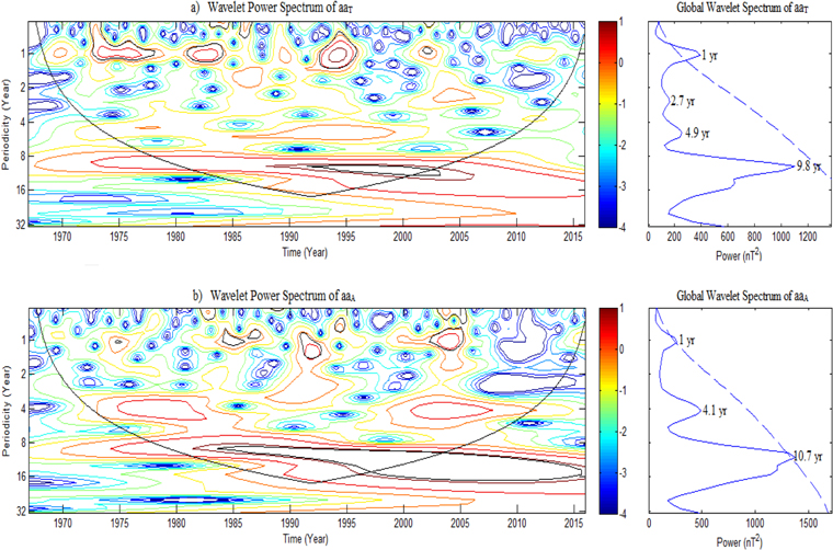
Figure 6. WPS and GWS of the geomagnetic index  , based on the HMF polarity, for the monthly averages of the toward (
 ; top plots) and away (
 ; bottom plots) sectors, over the period 1967–2016.
Download figure:
Standard image High-resolution image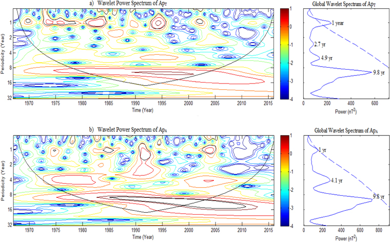
Figure 7. WPS and GWS of the geomagnetic index  , based on the HMF polarity, for the monthly averages of the toward (
 ; top plots) and the away (
 ; bottom plots) sectors, over the period 1967–2016.
Download figure:
Standard image High-resolution image
Figure 8. WPS and GWS of the geomagnetic index  , based on the IMF polarity, for the monthly averages of the toward (
 ; top plots) and the away (
 ; bottom plots) sectors, over the period 1967–2016.
Download figure:
Standard image High-resolution imageFigure 3 shows the WPS and the corresponding GWS of monthly averages of field magnitude for the toward ( ; upper plots) and the away (
 ; lower plots) HMF polarity sectors, over the period 1967–2016. It shows that the most prominent period in the GWS for
  and
and  is the solar activity cycle of 10.7 yr with nearly the same magnitude (or power). Also, the WPS of
  and
and  shows an increase of 1–2 yr periodicity during periods (1989–1994) for
  and (1989–1992) for
  . Furthermore, the two plots show an increase of the 2–4 yr periodicity during 1986–1995 for
  and 1974–1994 for
  . The observed periods include the quasi-biennial oscillation (QBO) around 2–2.5 yr and the quasi-triennial oscillation (QTO) around 3.5 yr. Also, during the periods 1977–1998 for
  and 1981–1998 for
  , the 4–8 yr periodicity shows a great and significant power compared to other times. One more variation of period ∼ 18–18.3 yr is observed during the period 1970–2016. The close-up view of the wavelet spectrum for
  and
and  shows that there is a coupling at some level between the 3.2–3.5, 10.7, and 18.3 yr variations. Therefore, both the WPS for
  and
and  showed nearly symmetrical power spectra. Finally, the 8–16 yr periodicity shows an increase in power during the whole interval, but it is under the COI. Table 2 displays the GWS and WPS periodicities of
  ,
,  ,
,  ,
,  ,
,  , and
, and  , based on the HMF polarity (
 or
or  ) over the period from 1967 to 2016. The powers of observed periodicities and their time periods are also tabulated.
Table 2.
GWS and WPS Periodicities for  ,
,  , and
, and  Based on the HMF Polarity Sense (Toward or Away) over the Period 1967 January–2016 December
| Parameter | Global Wavelet Periodicity | Power | WPS (95% C.L) | Time Periods | |
|---|---|---|---|---|---|
| Magnetic Field Magnitude |

|
1.8 yr | 3.464 | 1–2 yr | (1989–1994) |
| 3.2 yr | 3.406 | 2–4 yr | (1986–1995) | ||
| 5 yr | 4.75 | 4–8 yr | (1977–1998) | ||
| 10.7 yr | 66.22 | 8–16 yr | During the whole interval | ||
| 18.3 yr | 26.25 | ||||

|
3.5 yr | 6.456 | 0–1 yr | (1978–1979), (1989–1990) | |
| 10.7 yr | 67.27 | 1–2 yr | (1989–1992) | ||
| 18 yr | 32.47 | 2–4 yr | (1974–1994) | ||
| 4–8 yr | (1981–1998) | ||||
| 8–16 yr | During the whole interval | ||||
| Solar Plasma Velocity |

|
1 yr | 1.125 × 10⁴ | 0–1 yr | (1972–1977), (1984–1996) |
| 2.5 yr | 1.362 × 10⁴ | 1–2 yr | (1971–1977), (1990–1996) | ||
| 5.4 yr | 2.390 × 10⁴ | 2–4 yr | (1968–1977), (2002–2012) | ||
| 9.8 yr | 6.882 × 10⁴ | 4–8 yr | (1967–1982), (1986–2007) | ||
| 15.2 yr | 2.332 × 10⁴ | 8–16 yr | During the whole interval | ||

|
1.5 yr | 0.837 × 10⁴ | 0–1 yr | (1981–1984) | |
| 4.1 yr | 3.284 × 10⁴ | 1–2 yr | (1971–1975), (1991– | ||
| 9.8 yr | 6.081 × 10⁴ | 2–4 yr | 1996), (2002–2007) | ||
| 15.2 yr | 7.358 × 10⁴ | 4–8 yr | (1968–1983), (1998–2016) | ||
| 27.8 yr | 2.025 × 10⁴ | 8–16 yr | (1972–1988), (1995–2016) | ||
| During the whole interval | |||||
| Sunspot Number |

|
10.7 yr | 2.667 × 10⁵ | 4–8 yr | (1974–1999) |
| 30.3 yr | 0.197 × 10⁵ | 8–16 yr | During the whole interval | ||

|
10.7 yr | 2.643 × 10⁵ | 4–8 yr | (1973–2005) | |
| 30.3 yr | 0.166 × 10⁵ | 8–16 yr | During the whole interval | ||
Download table as: ASCIITypeset image
Figure 4 shows the WPS of the solar plasma speed according to the polarity of the HMF,  (upper plot) and
  (lower plot). The WPS of
  and
and  exhibited a wide variety of periodicities and time evolutions. The GWS of
  provides two significant peaks, within the 95% confidence level, at 9.8 and 15.2 yr, as well as at 1 and 9.8 yr, for
  . The other spectra are outside the 95% confidence level. Both spectra of
  and
and  are quite different, with a clear shift in time between both spectra. It can be seen that the spectral power of
  reaches maximum for a period of 9.8 yr during the whole period within the 95% confidence level, as well as at periods of 9.8 and 15.2 yr for
  . The most remarkable sign is the disappearance of the most prominent peak of solar activity, the 10.7 yr peak. In addition, the existence of a periodicity of 1 yr is obvious in
  spectra, and it shifted to a 1.5 yr variation in
  spectra.
On the other hand, we note that the strength of the 1–2 yr oscillation reaches nearly maximum power around 1971–1977 and 1991–1996 for both  and
and  . We note that the 1.7 yr period is a well-known period in cosmic-ray intensity observed at the Earth and might appear because of phenomena routed in the solar interior and could help with understanding the origin of the solar magnetic cycle (Valdes-Galicia & Mendoza 1998; El-Borie 2002; Kudela et al. 2002). Furthermore, for
  , the 2.5 and 5.4 yr oscillations are strong, where the maximum power of the 5.4 yr period occurred through 1970–1977 and 1986–2005, within the COI. Significant peaks were observed at a wavelength of 5.5–5.6 yr for the SW ion density (El-Borie 2002). Such variation is not shown in the
  spectra. Also, from Figure 4 it can be seen that the spectral powers of
  and
and  have a great magnitude throughout the period 8–16 yr during the whole period (Table 2). Also, the Hale cycle of ∼22 yr does not appear on the GWS within the 95% confidence level. The presence of periodicities in the solar-terrestrial parameters has been analyzed to observe their temporal average behavior using the GWS. The GWS of all significant peaks that appeared are listed in Table 2.
Figure 5 illustrates the WPS and GWS for  and
and  , for the monthly time series of SN during 1967–2016. The wavelet Morlet spectrum for the time series appears in the left panels, and the GWS appears in the right panels. In the WPS, two long-term variations can be seen. The well-known Schwabe (∼11 yr) variation is dominant and significant variation is seen in both the spectra (WPS and GWS). This period may be of interest from the point of view of solar physicists. The other observed long-term variation in SN is the 30.3 yr period during the whole period (appeared as a tiny periodicity). It is shown that the most remarkable period in the SN is the sunspot cycle with a period centered at 10.7 yr. Compared to the other periods, the 10.7 yr period possesses very large power during the whole time interval. The scaleogram shows that there is no significant appearance of peaks at 1–2, 2–4, and 4–8 yr. The spectra displays that there are no oscillations of the quasi-biennial (QBO) or the quasi-triennial (QTO). Thus, the WPS and GWS for
  and
and  have only one variation of 10.7 yr and another possible one of 30.3 yr (shown in the figures as a hint), with the same magnitude and location in both spectra, reflecting a symmetric power spectrum for both
  and
and  in the northern and southern hemispheres.
Velasco Herrera et al. (2018) studied the periodicities of 56 ground-level enhancement events in the time interval from 1966 to 2014. The results showed that the events occur preferentially in the positive phase of the QBO of 1.7 yr periodicity. They found quasi-regular periodicities of 10.4, 6.55, 4.12, 2.9, 1.73, 0.86, 0.61, 0.4 and 0.24 yr in ground-level enhancements. Some of these QBO periodicities may be interpreted as simply harmonics and overtones of the fundamental solar cycle. The QBO are broadly considered to be a variation of solar activity, associated with the solar dynamo process. Also, the intensity of these periodicities is more important around the years of maximum solar activity because the QBO periodicities are modulated by the solar cycle when the Sun is more energetically enhanced during activity maxima.
The period characteristics of SNs, SAs, and sunspot unit areas (SUAs) have been studied using the wavelet technique (Li et al. 2005). The results showed that the GWS of the three solar parameters resemble one another, all peaking at almost the same location. The result suggested that the variations of these three parameters exhibited very similar periodicities. For the SUAs, the most pronounced period was 10.13 yr, which is above the 95% confidence level. The same was found in the spectrum of the SNs. But for the SAs, only the ∼11 yr period was above the mean red-noise level. Li et al. (2014) studied the periodicities of the smoothed monthly hemispheric SNs, SA, and SAUs from 1945 to 2012. Their study showed that the northern solar hemisphere exhibited periodicity at 10.65, 10.72, and 10.96 yr for northern SNs, SAs, and SUAs respectively. However, periodicities at 10.84, 10.90, and 11.20 yr have been found for southern hemispheric SNs, SAs, and SUAs, respectively. These results showed that for each of the three parameters, the period of the Schwabe cycle for the southern hemisphere seems slightly longer than that for the northern hemisphere.
Since the discovery of the solar rotation and the 11 yr periodicity in the sunspots, the periodicities of solar activity and associated changes in the terrestrial environment have been studied extensively (e.g., Prabhakaran et al. 2002). The presented results provide numerous insights into the influence of solar-geomagnetic activities on HMF polarity. The most interesting result of the wavelet analysis of  , V, and
  is the appearance of statistical significance (with at least a 95% significance level) for mid-term and long-term oscillations. The study of the behavior of the N–S asymmetries for different solar phenomena indicated the existence of periodicities ranging 1–5 yr.
Also, the Hale cycle of ~22 yr does not appear on the GWS within the 95% confidence level. The presence of periodicities in the solar-terrestrial parameters has been analyzed to observe their temporal average behavior using the GWS. The GWSs of all significant peaks that appeared are listed in Table 2. Furthermore, the GWS and WPS revealed the existence of a strong peak of ∼10.7 yr in  and
and  , for two HMF polarities, than seen for the 22 yr period. The 22 yr periodicity is related to the changes in the polarity of the main solar magnetic field. In addition, the spectra of the velocities of solar plasma,
  and
and  , are sensitive to the ∼9.8 yr period observed in the WPS. The presence of QBO and QTO effects on spectra appeared as a change of the 2–4 yr periodicity in the WPS.
Figure 6 shows the WPS of the geomagnetic  index during 1967–2016. It is shown that the most prominent periods are the 10.7 yr period for
  and the 9.8 yr period for
  . Also, note that the periodicity of 1 yr showed an increase in magnitude during 1973–1984 and 1992–1996 for
  and 1982–1992 and 2000–2006 for
  , while the period 2–4 yr showed an increase in power throughout 2002–2006 for
  and 1999–2011 for
  . Finally, the period of 4.1–4.9 yr showed an increase in power during two the time intervals 1985–1990 for
  and 1973–1985 and 1998–2012 for
  .
.
Figure 7 shows the WPS and the corresponding GWS of monthly averages of geomagnetic  -index data. The well-known 9.8 yr periodicity variation is the dominant variation in both the spectra of
  and
and  . The 9.8 yr period possesses very large power during the whole interval. In the GWS of geomagnetic index
  , there are two signatures of smaller amplitudes; one corresponds to 1 yr and other corresponds to 4.1–4.9 yr. In addition, the WPS plot shows a significant power of the period 1–2 yr around 1985–1988 for
  and 1990–1993 and 2000–2006 for
  , while the 2–4 yr periodicity shows an increase in power during 1973–1994 and 2000–2009 for
  . Finally, the band around the 4–8 yr period in the wavelet spectrum is strong during 1975–2008 for
  .
.
Figure 8 shows the WPS of the geomagnetic activity  index. The spectra of
  are similar to those of
  and
and  , as shown in Figures 6 and 7. In the study of wavelet analysis of
  index, we observe that the period 8–16 yr has great power during the whole interval time for
  and
and  . Also, the most prominent peaks above COI are the sunspot cycles of 10.7 and 13.9 yr for the
  spectra and 9.8 yr for
  spectra. The GWS shows a double-peak structure for the spectrum of
  . The 1 yr periodicity reveals an increase in power during (1969–1984), (1993–1997), and (2010–2014). In addition, there is an obvious increase in period of 4–8 yr throughout (1972–1995) and (1999–2014). Furthermore, there is an increase in the periodicity of 4–8 yr during 1975–1990 compared to other times, which refers to the 4.1–4.9 yr periodicity for
  and
and  .
.
In conclusion, the wavelet technique used in our study provides an excellent means to determine the strength of quasi-periods in solar and geomagnetic activity parameters and their temporal evolutions. The GWS and WPS of solar plasma velocity  and the geomagnetic indices
  ,
,  , and
, and  , confirmed the presence of periodicity around 1–1.5, 4.1–4.9, and 9.8 yr, while the spectra of
  ,
,  ,
,  , and
, and  showed the effect of the solar activity cycle of period a 10.7 yr periodicity. The ∼11 yr solar cycle acts as an important driving force for such variations and is important for understanding the origin of different proxies of solar-geomagnetic variabilities.
The WPS of  ,
,  ,
,  ,
,  ,
,  , and
, and  represent the summary of the time evolutions of wavelet power for these parameters. For the geomagnetic
  ,
,  , and
, and  indices an oscillation of 1–2 yr has been observed at almost the same time intervals (see Table 3), confirming the results of Zossi et al. (2008), whereas they found that the main quasi-periodicities are 1.3–1.4 yr during solar cycles 20 and 22, as well as 1.6–1.7 yr for solar cycles 19 and 21. Using wavelet analysis in addition to Lomb/Scargle periodogram, Katsavrias et al. (2012) studied the frequencies of interplanetary magnetic field, plasma beta, Alfvén Mach number, SW speed, plasma temperature, plasma pressure, plasma density, and the geomagnetic indices Dst, AE, Ap, and Kp during the time interval 1966–2012. Mid-term (314 and 629 days) and long-term (4.1 and 8.2 yr) periodicities are found in solar plasma speed. In solar cycle 22 the periodicities were more clearly defined than in the rest of the observation period, with well-pronounced spectral peaks. Also, Valdes-Galicia & Mendoza (1998) showed a 1.7 yr periodicity in cosmic rays for solar cycle 21. Several authors have shown the presence of the 1.3 yr periodicity in geomagnetic and auroral activities (Szabo et al. 1995), with varying significant levels at different times. The periodicity in SW speed is speculated to be related to the topology of coronal holes or/and to the formation of open magnetic structures (Richardson et al. 1994; El-Borie 2002). These variations may be quite close to the Sun, likely in the SW source region (Gazis et al. 1995; Gazis 1996).
Table 3.
GWS and WPS Periodicities for  ,
,  , and
, and  , Geomagnetic Indices Based on the HMF Polarity Sense (Toward or Away) over the Period 1967 January–2016 December
| Parameter | Global Wavelet Periodicity | Power | WPS (95% C.L) | Time Periods | |
|---|---|---|---|---|---|
| Geomagnetic Index aa |

|
1 yr | 392.7 | 0–1 yr | (1973–1984), (1992–1996) |
| 2.7 yr | 160.6 | 1–2 yr | (1985–1988) | ||
| 4.9 yr | 253.3 | 2–4 yr | (2002–2006) | ||
| 9.8 yr | 1098 | 4–8 yr | (1985–1999) | ||
| 8–16 yr | During the whole interval | ||||

|
1 yr | 249 | 0–1 yr | (1982–1992), (2000–2006) | |
| 4.1 yr | 489.4 | 1–2 yr | (1990–1994) | ||
| 10.7 yr | 1372 | 2–4 yr | (1973–1983), (1988– | ||
| 4–8 yr | 1994), (1999–2011) | ||||
| 8–16 yr | (1972–1993) | ||||
| During the whole interval | |||||
| Geomagnetic Index Ap |

|
1 yr | 233.6 | 0–1 yr | (1969–1985), (1992–1996) |
| 2.7 yr | 87.34 | 1–2 yr | (1985–1988) | ||
| 4.9 yr | 134.3 | 4–8 yr | (1991–1998) | ||
| 9.8 yr | 574.8 | 8-16 yr | During the whole interval | ||

|
1 yr | 157.7 | 0–1 yr | (1982–1992), (2002–2006) | |
| 4.1 yr | 285.4 | 1–2 yr | (1990–1993), (2002–2006) | ||
| 9.8 yr | 728.2 | 2–4 yr | (1973–1994), (2000–2009) | ||
| 4–8 yr | (1975–2008) | ||||
| 8–16 yr | During the whole interval | ||||
| Geomagnetic Index Kp |

|
1 yr | 223.7 | 0–1 yr | (1969–1984), (1993– |
| 2.5 yr | 79.89 | 2–4 yr | 1997), (2010–2014) | ||
| 4.9 yr | 158.2 | 4–8 yr | (2003–2008) | ||
| 9.8 yr | 712.5 | 8–16 yr | (1973–1979), (1986–2000) | ||
| During the whole interval | |||||

|
1 yr | 125.5 | 0–1 yr | (1984–1988), (2002–2005) | |
| 4.1 yr | 252.8 | 1–2 yr | (1991–1993) | ||
| 10.7 yr | 796 | 2–4 yr | (1973–1982), (1999–2014) | ||
| 13.9 yr | 794.5 | 4–8 yr | (1972–1995), (1999–2014) | ||
| 8–16 yr | During the whole interval | ||||
Download table as: ASCIITypeset image
In addition, the WPS showed a periodicity of 2–4 yr for different parameters:  ,
,  ,
,  ,
,  , and
, and  . This periodicity includes the QBO and QTO. Several authors have identified a QBO in the geomagnetic activities. Among them, Olsen (1994) and Olsen & Kiefer (1995) postulated that the observed QBO in geomagnetic variations could be caused by the dynamo action of a QBO in lower thermospheric winds. Different periodicities around 0.5, 1, 2–2.5 yr (QBO), 3.5 (QTO), 5.5 yr (2nd harmonic of 11 yr cycle), and 11 yr cycles were found in a geomagnetic storm represented by Dst ≤ 50 nT during the period 1957–2004 (Zossi et al. 2008).
Kane (2005) focused on analyzing the QBOs present in solar, interplanetary, and terrestrial parameters. A QBO that is strong near solar maximum appeared for solar indices, the cosmic rays observed on Earth being indicative of a similar distribution of peaks. Based on a study of geomagnetic storms, Gonzalez et al. (1990, 1993) found that the yearly distribution of storms presents two peaks around the solar maximum: one at the solar maximum or slightly earlier, and the other in the early part of the descending phase. The average separation of these peaks is between three and four years. This may be related to a similar dual-peak structure provided by the intensity of certain coronal processes, as explained by Gonzalez et al. (1996). Thus, there exist mechanisms in different stages of the solar cycle that explain this periodicity. El-Borie (2002) detected a similar oscillation in the  index. This quasi-periodic fluctuation is attributed to the change in high-speed SW streams associated with sector boundary passages rather than the dual-peak distribution of intense geomagnetic storms.
Katsavrias et al. (2016) used the cross-wavelet transform (XWT) and wavelet coherence (WTC) to examine the relationship between transient and recurrent phenomena, interplanetary coronal mass ejections (ICMEs) and the corotating interaction regions (CIRs), and the corresponding magnetospheric response represented by geomagnetic indices (Dst and AE) within solar cycle 23. The study showed that the CIRs modulate this geomagnetic response during the rise and decline phases, while ICMEs modulate the response during the maximum of the cycle and the unusual active period of 2002–2005; the phase-relationship varies strongly in all cases for both drivers. In addition, a periodicity of ≈1.3–1.7 yr of the CIR time series seemed to be the dominant driver for both the Dst and AE indices throughout solar cycle 23. Moreover, in the band around 4.1–4.9 yr in geomagnetic  ,
,  , and
, and  indices for different times. Echer et al. (2004) observed the 5 yr periodicity in
  index. It was observed in SW speed and in the intensity of the interplanetary magnetic field
  (Rangarajan & Barreto 2000). Significant peaks were found at a wavelength of 5.5–5.6 yr for the SW ion density (El-Borie 2002). Djurović & Pâquet (1996) considered a periodicity of 5.5 yr in solar activity, indicated by
  , is the second harmonic of the 11 yr cycle.
Finally, a very small (or a tiny) periodicity close to 30 yr is detected in WPS in SN in both WPS and GWS. Singh & Badruddin (2014) observed different periodicities in the SNs, one of them 38.6 yr. In addition, they observed a periodicity of 30 yr in the geomagnetic aa-index. It is noteworthy that a periodicity of around 30 yr (the so-called three cycle quasi-periodicity) in cosmic-ray data was reported earlier by Ahluwalia (2012) and Perez-Peraza et al. (2012). On the other hand, Sunkara & Tiwari (2016) applied the wavelet spectral analysis on the Western Himalayan temperature variability records for 125 yr (1876–2000), showing a strong high power at ∼62, 32–35, 11, 5 and 2–3 yr, and suggesting a strong influence of solar–geomagnetic–ENSO effects on the Indian climate system. Furthermore, a prominent signal corresponding to a 33 yr periodicity in the tree-ring record was found, suggesting the Sun-temperature variability link is probably induced by changes in the basic state of the Earth's atmosphere.
4. Summary and Conclusions
The irregularity of solar activity phenomena (such as; HMF, SNs, SAs, solar radio flux, etc.) between the northern and southern solar hemispheres is referred to as the N–S asymmetry. The N–S asymmetry of HMF polarity between the northern and southern hemispheres has been considered. The impact of HMF polarity on monthly average observations of  ,
,  ,
,  ,
,  ,
,  , and
, and  over the period 1967–2016 has been studied. The data have been classified into two groups according to HMF polarity (
 or
or  ). The monthly average of the
  and
and  groups has been determined for each parameter. We perform the wavelet power spectra technique to study and examine the dependence of solar, plasma, and geomagnetic parameters' oscillations on the HMF polarities and compare the obtained results for solar, plasma, and geomagnetic indices during the considered period. Our findings are summarized as follows:
- (1)Both the WPS for
 and nearly showed a symmetrical power spectra distribution. The wavelet spectrum for and displayed a coupling at some level between the 3.2–3.5, 10.7, and 18.3 yr of variations.
 - (2)The WPS of and exhibited a wide variety of periodicities and their time evolutions. The global wavelet spectrum for provided two significant peaks, within the 95% confidence level, at 9.8 and 15.2 yr, as well as at 1 and 9.8 yr, for . In addition, the existence of a periodicity of 1 yr is obvious for spectra and it shifted to a 1.5 yr variation in spectra. For the spectra of , the disappearance of the most prominent peak of solar activity, the 10.7 yr peak and the Hale cycle of ∼22 yr, is a remarkable sign.
- (3)WPS and GWS for and displayed two long-term variations, one variation of 10.7 yr and another possible one of 30.3 yr, with the same magnitude and location in both spectra, reflecting symmetric power spectra for both and in the northern and southern hemispheres.
- (4)For the spectra, the most prominent period is the 10.7 yr for and 9.8 yr for . Also, the well-known 9.8 yr periodicity variation is the dominant variation in the spectra of and . On the other hand, within the COI, the periodicities of 10.7 and 13.9 yr are observed for the spectra and 9.8 yr for spectra. The GWS showed a double-peak structure for the spectrum of .
- (5)Both the GWS and WPS of solar plasma velocity and geomagnetic indices , , and , confirmed the presence of periods around 1, 4.1–4.9, and 9.8 yr, while the spectra of , , , and showed the effect of the solar activity cycle of period 10.7 yr.
- (6)The presented results provide numerous insights into the influence of solar-geomagnetic activities. The most interesting result of the wavelet analysis of, V, and R is the appearance of statistical significance (with at least 95% significance level) for mid-term and long-term oscillations. The study of the behavior of the N–S asymmetries for different solar phenomena indicated the existence of periodicities ranging 1–5 yr.


We gratefully acknowledge the use of the OMNI data explorer from the National Space Science Data Centre (http://www.omniweb.gsfc.nasa.gov). We also gratefully acknowledge Wilcox Solar Observatory (WSO) for providing the HMF polarity data. We are thankful to C. Torrence and G. Compo for providing the wavelet software package. Finally, we thank the referee for valuable comments and suggestions.