


Abstract
Type Ia supernovae, calibrated by classical distance ladder methods, can be used, in conjunction with galaxy survey two-point correlation functions, to empirically determine the size of the sound horizon rs. Assumption of the ΛCDM model, together with data to constrain its parameters, can also be used to determine the size of the sound horizon. Using a variety of cosmic microwave background (CMB) data sets to constrain ΛCDM parameters, we find the model-based sound horizon to be larger than the empirically determined one with a statistical significance of between 2σ and 3σ, depending on the data set. If reconciliation requires a change to the cosmological model, we argue that change is likely to be important in the two decades of scale factor evolution prior to recombination. Future CMB observations will therefore likely be able to test any such adjustments; e.g., a third-generation CMB survey like SPT-3G can achieve a threefold improvement in the constraints on rs in the ΛCDM model extended to allow additional light degrees of freedom.
Export citation and abstract BibTeX RIS
1. Introduction
Classical distance ladder (CDL) approaches using Cepheids and supernovae (SNe; Riess et al. 2018b, hereafter R18) find higher Hubble constant estimates than those derived from cosmic microwave background (CMB) data that assume the standard cosmological model, ΛCDM (Planck Collaboration VI 2018). The statistical significance of this discrepancy has grown over time with fairly steady progress on the distance ladder (Riess et al. 2009, 2011, 2016) and with a sudden jump in precision of the ΛCDM prediction with the first release of the Planck cosmology data in 2013 (Planck Collaboration XVI 2014). Comparing the R18 value of H0 = 73.52 ± 1.62 km s−1 Mpc−1 with the value inferred from Planck CMB temperature and polarization power spectra plus CMB lensing, assuming ΛCDM, H0 = 67.27 ± 0.60 km s−1 Mpc−1, there is a 3.6σ discrepancy (Planck Collaboration VI 2018).
Along with the reduction of statistical errors in the Cepheids-plus-SNe determination of H0, other supporting evidence in favor of a high value of H0 has been growing as well. A number of independent analyses of the data have served to largely confirm the conclusions of R18 (Efstathiou et al. 2014; Cardona et al. 2017; Zhang et al. 2017; Feeney et al. 2018; Follin & Knox 2018). Despite claims that the CDL H0 departs significantly from the cosmic mean H0 due to a local void, Wu & Huterer (2017) showed that within ΛCDM, the sample variance in the R18 measurement is only 0.3 km s−1 Mpc−1, or 0.2σ. In addition, Birrer et al. (2019) provided the latest inference of H0 from the H0LiCOW (Suyu et al. 2017) collaboration's use of strong-lensing time delays (SLTDs):  km s−1 Mpc−1. Combining the result of this completely independent probe of the distance–redshift relation at low redshift with that from R18 results in a 4.1σ discrepancy with the Planck result quoted above. Finally, the tip of the red giant branch distance method shows consistency with Cepheid distances to a handful of SN host galaxies (Jang & Lee 2017; Hatt et al. 2018a, 2018b).
Recently, Shanks et al. (2019) claimed that corrections applied to the Gaia data (Lindegren et al. 2018) in the R18 analysis have introduced significant systematic error, a claim that has sparked a debate (Riess et al. 2018a; Shanks et al. 2018). We simply point out here that the Riess et al. (2016) result of H0 = (73.24 ± 1.74) km s−1 Mpc−1 makes no use of Gaia data and is thus immune to this controversy, while also being nearly as discrepant from the ΛCDM–plus–CMB-inferred values.
The case against systematic errors in CMB data as the source of this discrepancy is very strong. First of all, the result from Planck is robust to the choice of frequency channels (Planck Collaboration et al. 2016), arguing against foreground modeling or any channel-specific systematic errors as a source of bias in the H0 inference. Further, the consistency of Planck measurements with the Wilkinson Microwave Anisotropy Probe (WMAP) on large angular scales (Planck Collaboration et al. 2014) and the 2500 deg2 SPT-SZ measurements on small angular scales (Aylor et al. 2017; Hou et al. 2018) also argues against any significant systematic errors on all angular scales relevant for the determination of cosmological parameters from Planck data.
Additionally, the conclusion of a low H0 from CMB data and the assumption of ΛCDM can be reached without the use of Planck data. The inverse distance ladder results (Percival et al. 2010; Heavens et al. 2014; Aubourg et al. 2015; Cuesta et al. 2015; Bernal et al. 2016a; DES Collaboration et al. 2018; Verde et al. 2017b; Feeney et al. 2019; Joudaki et al. 2018; Lemos et al. 2018) also show that the combination of measurement of the baryon acoustic oscillation (BAO) feature in galaxy surveys, Type Ia supernova (SN Ia) observations, and CMB data with or without Planck (e.g., WMAP9; Bennett et al. 2013) lead to low (Planck-like) values of H0. Finally, Addison et al. (2018) pointed out that, assuming the ΛCDM model and using BAO data and light-element abundance measurements as constraints on the baryon-to-photon ratio, one infers a Planck-like value of H0, i.e., without using any CMB anisotropy data. The above results indicate that systematic errors in CMB data, and Planck CMB data in particular, are not the major driver of the discrepancies in inferences of H0.
Recently, some works in the literature have proposed solutions both pre- and post-recombination to address the H0 discrepancy. For example, Karwal & Kamionkowski (2016), Evslin et al. (2018), and Poulin et al. (2018) proposed the existence of an early dark energy that reduces the size of the sound horizon, subsequently increasing the CMB-inferred value of H0; Lin et al. (2019) proposed a modified gravity solution at the time of recombination; and Chiang & Slosar (2018) altered the duration of the recombination to reduce the tension between CMB and CDL results. On the other hand, Di Valentino et al. (2016, 2017) and Joudaki et al. (2017) used an extended parameter space and pointed out that an interacting phantom-like dark energy with an equation of state wDE < −1 can also reduce the tension in H0 measurements.
In this paper, to further explore what can and cannot explain this discrepancy, we follow Bernal et al. (2016b) and use the sound horizon rs, rather than H0, as the point of comparison between CDL and ΛCDM-based estimates. With this approach, the BAO data are on the CDL side: Cepheids calibrate SNe Ia, which are then used to determine distances to redshifts for which BAO measurements of the angular size of the sound horizon exist, thereby revealing the size of the sound horizon. We also note that SLTDs can be used to calibrate the BAO measurements, so we convert the H0LiCOW result into a sound horizon constraint. For a more comprehensive use of data sensitive to distances and the expansion rate at low redshifs (z ≲ 1), see, e.g., Bernal & Peacock (2018), which includes the use of "cosmic clocks."
We find use of the sound horizon as a point of comparison to be a particularly useful way of examining the data for several reasons. First, there is added insensitivity with this method to extreme changes in the z < 0.1 cosmology, since one does not need to extrapolate to z = 0, circumventing issues with peculiar velocities brought up by Shanks et al. (2019). Second, the ΛCDM predictions for the sound horizon are more robust than those for H0. Third, as with the inverse distance ladder, this approach clarifies that reconciliation cannot be delivered by altering cosmology at z < 1. Fourth, it serves to clarify that the reconciliation of distance ladder, BAO, and CMB observations via a cosmological solution is likely to include a change to the cosmological model in the two decades of scale factor evolution prior to recombination. Finally, σ(rs)/rs from CMB data, assuming that ΛCDM is four times smaller than the σ(H0)/H0 from the same data and assumed model.
Since Bernal et al. (2016b), we have new SN data available (Scolnic et al. 2018), an updated SN absolute luminosity calibration (R18), and results from the final data release from Planck (Planck Collaboration VI 2018). We examine the tension in rs given these most recent data. As mentioned above, SLTDs can also be used to calibrate the distance to the BAO redshifts. So we also use the latest H0LiCOW results (Birrer et al. 2019) to produce a constraint on rs.
We find that the CDL-inferred sound horizons are in 2σ–3σ tension with ΛCDM-determined ones.9 While a statistical fluke could explain this discrepancy, we believe there is sufficient evidence to motivate the exploration of cosmological solutions. In Section 4, we argue that if there is to be a cosmological solution to the discrepancies in rs values, it is likely to be significantly different from ΛCDM in the two decades of scale factor growth prior to recombination. Such model changes are likely to lead to predictions testable with future CMB data. We examine the rs predictions in the case of a two-parameter extension of the standard cosmological model and forecasts for rs errors in these extended model spaces given the survey to come from SPT-3G, a third-generation camera outfitted on the South Pole Telescope (Benson et al. 2014; Bender et al. 2018).
2. Models and Data
We present here the empirical CDL approach to determining the sound horizon scale, rs, and then the more cosmological model–dependent approach. Although the former also requires modeling, we demonstrate with a parametric spline model for the history of the expansion rate that the results are at most only mildly dependent on cosmological model assumptions. We also describe how we use the recent H0LiCOW results (Birrer et al. 2019) to determine rs.
2.1. rs Using CDL
We describe the formalisms to determine rs empirically in this section. For this purpose, we use the BAO data from the BOSS survey (Alam et al. 2017), SN data from the SN Ia Pantheon sample (Scolnic et al. 2018), and Cepheid data from R18.
The sound horizon leaves its imprint on the galaxy distribution as a peak in the galaxy two-point correlation function at rs, the comoving size of the sound horizon.10 In redshift space, with galaxy positions recorded in z and angular position on the sky, the sound horizon scale maps into (Δz)s = H(z)rs (the difference in redshift between two galaxies with a line-of-sight separation rs) and θs(z) = rs/DA(z) (the angular separation of two galaxies separated by rs perpendicular to the line of sight), where DA(z) is the comoving angular diameter distance. Thus, BAO surveys fundamentally constrain these two quantities, and analyses often summarize the constraints as constraints on H(z)rs and DA(z)/rs.
The SNe Ia are used as "standardizable" candles that, after suitable data-dependent corrections, can be reduced to a corrected apparent magnitude with a signal modeled by

where i runs over SNe; the first term on the right is a global, SN-independent, corrected absolute magnitude; and the second and third terms just follow from the inverse square law for fluxes and the definitions of apparent and absolute magnitudes, with DL the comoving luminosity distance.
Neglecting, for the moment, the BAO constraints on H(z)rs, the BAO and SN constraints are very similar. Both the BAO and SN data determine a distance–redshift relationship up to some global scaling factor. In the BAO case, the scaling factor is rs, and in the SN case, we could take it to be lSN ≡ 10−(M + 19)/5 Mpc.11 The two different distances are also very simply related, assuming conservation of photon number, via DA(z) = DL(z)/(1 + z).
We can relate these observable distance ratios to H(z), assuming a negligible mean spatial curvature, via
with βBAO ≡ c/(rs H0) and βSN ≡ c/(lSNH0).
Finally, there are the Cepheids. The Supernovae, H0, for the Equation of State of Dark energy (SH0eS; Riess et al. 2018b) program has used Cepheids in 19 different host galaxies with observed SNe Ia to calibrate the mean SN absolute magnitude. Rather than directly using that calibration, we use the value of H0 that results from the calibration. As one can see in the equations above, the SN data themselves are sensitive to the combination βSN ≡ c/(lSNH0), so specifying H0 allows one to determine lSN; i.e., it allows for a calibration of the SN distance measurements.
We use the BAO, SN, and Cepheid data as just (generically) described to infer rs, performing our analyses with two different model spaces. One is ΛCDM with
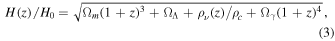
where

here ρν(z) is calculated for a neutrino background with a temperature today of Tν,0 = 2.725 K (4/11)1/3, two m = 0 mass eigenstates and one with mass mν with a default value of 0.06 eV. Ωγ the energy density, in units of the critical density, in a blackbody of photons with temperature Tγ,0 = 2.725 K. The complete set of parameters of this model can be taken to be {βBAO, βSN, H0, Ωm}. Note that the sound horizon scale is a derived parameter given by rs = c/(βBAOH0).
The other model we call the spline model. For this model, following Bernal et al. (2016b), H(z)/H0 is determined by H(z) at five locations in z and cubic spline interpolation. The complete set of parameters for the spline model is {βBAO, βSN, H0, H1, H2, H3, H4}, where Hi ≡ H(zi) with z0 = 0, z1 = 0.2, z2 = 0.57, z3 = 0.8, and z3 = 1.3, for which we assume a uniform prior over the region with H(zi) > 0. These were the redshift points used by Bernal et al. (2016b). We also consider a slightly different choice to check robustness in Section 3.1.2.
We note that the spline model results are not completely free of cosmological assumptions, as the relationship between H(z) and DA(z) depends on curvature. If it were not for the BAO constraints on H(z), then our spline model–based inferences of rs would not have any dependence on curvature, as our H(z) parameters can just be thought of, in that case, as a means of parameterizing DA(z). The reconstructed H(z) would have curvature dependence, but the recovered rs would not. The inclusion of the BAO constraints on H(z) breaks that degeneracy in curvature and brings some dependence of the inferred rs on assumptions about curvature. We will discuss this dependence in Section 3.
To perform joint analyses of the three data sets, we form a log likelihood  (natural log of the likelihood), given by

We now briefly describe each of these likelihoods in turn.
The log likelihood  has the BAO means and error covariance matrix described in the BOSS collaboration paper (Alam et al. 2017) for DA(z)/rs and H(z)rs at the effective redshifts z = 0.38, 0.51, and 0.61. These data points are plotted as red squares in Figures 1 and 2 as constraints on DA(z) and H(z), given a fiducial value of rs.
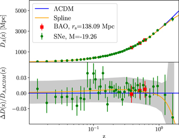
Figure 1. Comoving angular diameter distance measurements, DA(z), together with best-fit models. The BAO results have been converted from DA(z)/rs to DA(z) by assumption of rs = 138.09 Mpc. The SN distance moduli have been converted to DA(z) assuming M = −19.26. In the residuals panel, ΔDA(z) = DA(z) − DA,ΛCDM(z), where DA,ΛCDM(z) is the comoving angular diameter distance for the best-fit ΛCDM cosmology. The gray band shows the 68% confidence interval for the spline model.
Download figure:
Standard image High-resolution imageWe do not include any other BAO data, such as that from the 6df galaxy survey (Beutler et al. 2011) or a BOSS DR12 Lyα absorption cross-correlation analysis (du Mas des Bourboux et al. 2017). While they provide useful consistency tests of the standard cosmological model, they are not as precise as the BOSS galaxy constraints (Alam et al. 2017), and some are also at redshifts greater than the highest redshifts for which we have SN distance estimates, rendering them uninformative for our main purpose.
To construct the likelihood for SNe, we use the Scolnic et al. (2018) data set. They reported the redshift-binned estimates of corrected B-band SN apparent magnitudes, corrected to improve the approximation m = μ(zβ)+M for some global M, where μ(zβ) is the distance modulus for redshift zβ. We thus model the data as

The absolute magnitude M is the more usual way of specifying the calibration of the SNe. Taking lSN introduced above to have the fiducial value of 1 Mpc for a fiducial value of M = −19.3 (for specificity), Equation (6) can be rewritten to swap in lSN for M:

We form a likelihood that is Gaussian in the apparent magnitudes, with covariance matrices that include the statistical and systematic errors as reported in Scolnic et al. (2018). The data points are plotted as green circles in Figure 1 as constraints on DA(z) = DL(z)/(1 + z) for a fiducial value of M.
For the "Cepheids" log likelihood, we take

where H0 is our model Hubble constant in km s−1 Mpc−1 and the numbers in the likelihood are from the R18 measurement H0 = 73.52 ± 1.62 km s−1 Mpc−1. Note that, just like for rs with the BAO data, lSN is a derived parameter given by c/(βSNH0). The SN absolute magnitude parameter M can likewise be derived from lSN.
2.2. rs and SLTDs
We also consider SLTD data (Birrer et al. 2019) as a means of calibrating the BAO. A given SLTD system is sensitive to the ratio DdDs/Dds, where Dd is the distance to the lens (typically near z ∼ 0.5), Ds is the distance to a lensed quasar (typically near z ∼ 1.5), and Dds is the distance between the two. This quantity is inversely proportional to H0, and, in ΛCDM, its dependence on the exact shape of H(z) (given largely by Ωm) is weak enough to, even with very weak priors on the matter density, produce a strong constraint on H0. We can thus use this constraint to anchor the BAO point instead of the Cepheids without any other additional external data. In practice, we simply combine the constraint on βBAO, which we get from SNe and BAO with the H0 reported by Birrer et al. (2019), propagating Gaussian error bars in quadrature.
We note that this analysis is approximate because we have not jointly analyzed the data sets; improved constraints on the matter density from the SNe+BAO data could further tighten the H0LiCOW result. However, this effect is likely to be small given the weak dependence on the Ωm prior reported by Birrer et al. (2019). Note that this analysis does assume ΛCDM, in particular that the shape of H(z) follows the expectation from ΛCDM between today and the quasar redshifts of z ∼ 1.5. While the SNe strongly constrain the shape at somewhat lower redshifts, there is, at least in theory, the possibility that the H0LiCOW inference of H0 and thus our corresponding rs inference could be somewhat thrown off by a change to H(z) right around z ∼ 1.5. We have not attempted a joint spline fit of SNe+BAO+H0LiCOW, but such a test could reveal to what extent this is a possibility (although, of course, the H0LiCOW and Cepheid determinations of H0 are already in good agreement, arguing against this possibility).
2.3. rs from ΛCDM-plus-CMB Data
We have just reviewed how one can infer rs in an empirical manner using the CDL. Here we describe how one can adopt a model and directly calculate rs. The comoving size of the sound horizon is given by

where cs(a) is the sound speed as a function of the scale factor and ad is the scale factor at the end of the baryon drag epoch. In the ΛCDM model, rs is completely determined by the baryon-to-photon ratio for its influence on ad and cs(a) and the matter density ωm ≡ Ωmh2 for its influence on ad and H(a). With these parameters constrained, or any other relevant parameters there might be in extended model spaces, one can then calculate a constraint on rs.
We use the CMB data sets from the Atacama Cosmology Telescope (ACTPol; Louis et al. 2017), Planck (Planck Collaboration VI 2018), the South Pole Telescope: SPT-SZ (Aylor et al. 2017) and SPTpol (Henning et al. 2018), and the WMAP (Bennett et al. 2013). We look at subsets of the Planck data as well. Significant constraints on rs come from each of the three dominant power spectra,  , and
, and  , as well as from
  at l < 800 and
  at l > 800.
3. Results and Discussion
Before presenting the constraints on rs from the different methods described in Section 2, in Figures 1 and 2, we display the BAO and SN data as they constrain DA(z) and H(z). For these figures, we assume the fiducial values rs = 138.09 Mpc and M = −19.26, which are the best-fit values for the spline model parameter space described in Section 3.1.2 given the BAO, SN, and Cepheid data. We choose the best-fit values from the spline model, as opposed to the ΛCDM model, primarily for specificity and secondarily in order to have less model dependence in the resulting distance estimates.
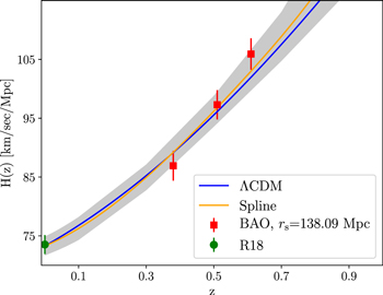
Figure 2. Expansion rate measurements together with best-fit models. The BAO data have been converted to H(z) by assumption of rs = 138.09 Mpc. The gray band shows the 68% confidence interval for the spline model.
Download figure:
Standard image High-resolution imageExamining the residuals from these fits in Figures 1 and 2, we see no obvious problems for either the ΛCDM or spline modes. For the ΛCDM model, we find for the best fit  and
and  , summing to
  for 43 degrees of freedom (40 SN data points, six BAO data points, and three parameters, not counting H0). For the spline model, we find the best fit
  and
and  , with
  for 40 degrees of freedom (six parameters, once again not counting H0).
Now we turn to results reporting the inferred value of rs using the CDL approach from the ΛCDM and spline models in Section 3.1. This is followed by the results obtained using CMB data for the ΛCDM model in Section 3.2. Next, we discuss the 2σ–3σ tension in the value of rs obtained from these two methods in Section 3.3. In Section 3.4, we look at a couple of model extensions and forecast the expected constraints on rs that can be obtained by combining Planck results with SPT-3G (Benson et al. 2014), a stage 3 CMB temperature and polarization survey. Finally, in Section 4, we argue that if the origin of the discrepancies is cosmological, the cosmological solution must make its important changes at times prior to recombination.
3.1. CDL-based Constraints
We begin our discussion with our first result of the H0 constraint (which we refer to as "Cepheids"; R18) used for calibrating the Pantheon binned distance moduli ("SNe"; Scolnic et al. 2018), which in turn are used to calibrate the BAO distance and H(z) constraints from BOSS galaxies ("BAO"; Alam et al. 2017). The CDL-based rs results are shown as blue circles in the top panel of Figure 3.
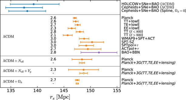
Figure 3. Sound horizon determinations from existing data (filled symbols) and forecasts (open symbols). The numbers down the middle give the difference with the Cepheids+SNe+BAO spline model result for rs in units of the standard deviation, with the standard deviation computed via quadrature sum. We see that the CDL constraints (top panel) on rs come out systematically lower than the ΛCDM-based constraints (biggest panel). The three model extensions considered in the three remaining panels do not significantly weaken the discrepancy. The code and data for this figure are available.12
Download figure:
Standard image High-resolution image
3.1.1. CDL+ΛCDM
First, we have assumed the ΛCDM model—using it to provide the parameterized shape of H(z)/H0. We find

As a point of comparison, we mention a result from Addison et al. (2018). They take a more comprehensive set of BAO data, including constraints at lower redshift from galaxy surveys (Beutler et al. 2011; Ross et al. 2015) and higher redshift constraints from BOSS Lyα (Font-Ribera et al. 2014; Delubac et al. 2015; Bautista et al. 2017) and find, from the BAO data themselves, assuming the ΛCDM model, that H0rs = (10,119 ± 138) km s−1. Combining this with the R18 result for H0, it becomes

This result is nearly the same, in mean and standard deviation, as our own CDL+ΛCDM result. The lack of reduction in uncertainty, despite the much greater amount of BAO data, is due in part to the lack of use of the SN Ia data, which increases the uncertainty in Ωm and therefore the shape of DA(z). The other important factor in the lack of reduction is that the BOSS galaxy data are unmatched in precision.
Our second CDL+ΛCDM result comes from replacing Cepheids (R18) with the SLTD data from H0LiCOW (Birrer et al. 2019), as explained in Section 2.2. From our SN Ia + BAO data, we have βBAO ≡ c/(rsH0) = 29.7 ± 0.37. Combining this with  km s−1 Mpc−1 from Birrer et al. (2019), we find

That uncalibrated SN, combined with BAO data, put a strong constraint on the product rsH0 (=c/βBAO), previously mentioned in Verde et al. (2017b).
3.1.2. CDL+Spline
To explore the model dependence of the CDL method for rs inference, we now drop the assumption of ΛCDM for parameterization of the shape of H(z)/H0 and replace it with our spline model. Because our BAO results span such a small range of redshift, we can expect that there is very little sensitivity of the inferred rs to the choice of parameterization, as long as it is not varying rapidly on redshift intervals comparable to the redshift span of the BAO measurements. With the four-parameter model described in the previous section, we indeed find a very similar result to the ΛCDM result:

That this sound horizon result is a little bit larger is consistent with what we see in the residuals panel of Figure 1. Namely, the SN data largely sit above the ΛCDM best-fit curve in the redshift interval with the BAO data. The increased freedom of the empirical model reduces the influence of the SNe outside of this redshift range, boosting D(z) in this interval with the result that rs is slightly larger. Note, though, that statistically, this is a very small shift of less than 0.2σ.
More importantly, because the ΛCDM and spline results for rs are basically the same, including in the uncertainty, we can conclude that the CDL sound horizon determination is highly model-independent. In particular, it is, at most, very weakly dependent on any assumptions about the shape of the distance–redshift relationship. As a further check, we performed an analysis with spline points moved to z = {0, 0.2, 0.5, 0.8, 1.1} away from our baseline z = {0, 0.2, 0.57, 0.8, 1.3} (see Section 2.1) and obtained rs = 137.7 ± 3.60 Mpc, indicating that our results are not highly sensitive to the choice of pivotal redshift points.
Before closing this subsection, we comment on the dependence of the CDL result for rs on curvature. Using R16 for the H0 constraint, Betoule et al. (2014) for the SN Ia data, and the same BOSS BAO data, Verde et al. (2017b) found, also for a phenomenological parameterization of H(z), that rs = 138.5 ± 4.3 Mpc assuming ΩK = 0. This is consistent with our result to within 0.2σ. When they marginalized over ΩK, they found rs = 140.8 ± 4.9 Mpc. This is an ∼0.5σ shift, which indicates that were we to relax our zero curvature assumption, it might have some impact on the significance of our results. We caution against seeing this small shift as possibly leading to a resolution between the CMB and CDL data. To get the full magnitude of this shift requires the curvature to be quite far from zero. The Verde et al. (2017b) constraint on Ωk in this analysis is ΩK = 0.49 ± 0.64. Such a large value of Ωk is highly disfavored by CMB data; in the ΛCDM+Ωk model, the Planck temperature and polarization power spectra lead to ΩK = −0.044 ± 0.034.
3.2. ΛCDM-based Constraints with and without CMB Data
We now turn to the model-based determinations of the sound horizon, focusing first on the ΛCDM model results. To examine the robustness of sound horizon determination, we show results for many choices of CMB data sets (orange circles in the biggest panel of Figure 3). We see some scatter in these inferences of rs, with all of them between 2σ and 3σ larger than the spline-based CDL result.
A curious feature of the scatter in the ΛCDM results is that those data sets that lead to lower values of H0, such as using Planck temperature power spectrum (TT) data restricted to l > 800 (+lowE), which are thus more discrepant with the CDL value of H0, also lead to values of rs that are less discrepant with the CDL, and vice versa. This pattern can be understood as follows. First, recall that the comoving size of the sound horizon is given by Equation (9), which, in the ΛCDM model, depends only on the baryon-to-photon ratio and the matter density ωm. The fluctuations in ΛCDM-based rs inferences from CMB data are almost entirely driven by fluctuations in ωm. The short explanation for the positive correlation between H0 and rs fluctuations is that upward fluctuations in ωm drive both rs and H0 downward.
The positive correlation between rs and H0 can be understood as follows. If the radiation density were completely negligible for the calculation of the sound horizon, then, from the Friedmann equation, δH(a)/H(a) ∝ 0.5δωm/ωm, so we have δrs/rs ∝ −0.5δωm/ωm. The radiation softens this response to closer to δrs/rs ∝ −0.25δωm/ωm (Hu et al. 2001). To keep the angular size of the sound horizon fixed (in order to stay at a high-CMB data likelihood), we have for the distance from here to z = zd, δD/D = δrs/rs = −0.25δωm/ωm. For the model to achieve this softened response of the distance to the matter density (softened to a −0.25 exponent as opposed to −0.5), there has to be a fluctuation in the dark energy density that is anticorrelated with the matter density fluctuation, with the result that δH0/H0 has the same sign from δrs/rs, as also explained in Hou et al. (2014). Perhaps of particular note regarding this positive correlation between rs and H0 fluctuations is that those data sets that are somewhat more consistent with the CDL for H0 than is the case for Planck are less consistent with the CDL for rs. This is the case for Planck TT (l < 800), WMAP9+SPT+ACT (Calabrese et al. 2017), SPT-SZ (Aylor et al. 2017), and SPTpol (Henning et al. 2018). These fluctuations toward higher H0, if they go far enough to reconcile with R18, end up being discrepant with BAO data (given the ΛCDM model), as noted in Hou et al. (2014).
While the above results indicate robustness to the choice of the CMB data, Addison et al. (2018) demonstrated that rs can be estimated, assuming ΛCDM, without any CMB anisotropy data at all. They used a combination of BAO data and constraints on ωb from inferences of the primordial abundance of deuterium relative to hydrogen (D/H; Cooke et al. 2016). Within ΛCDM, rs is entirely determined by ωm and ωb via Equation (9). Given the assumption of ΛCDM, the BAO data can be used to constrain ωm. This constraining power arises from the degeneracy-breaking power of separately parallel and perpendicular constraints at several different redshifts. The primordial D/H ratio resulting from big bang nucleosynthesis (BBN) is highly sensitive to the baryon-to-photon ratio and can therefore be used to estimate ωb. Addison et al. (2018) combined galaxy and Lyα forest BAO with a precise estimate of the primordial deuterium abundance (Cooke et al. 2016) to find rs = 151.6 ± 3.4 Mpc. The BAO+BBN-based rs is shown in Figure 3 in purple (rather than orange like CMB), as it relies on BAO data that have also been used for the CDL determination and whose interpretation is dependent in this case on late-time assumptions of the ΛCDM model. This result, like the CMB-based estimates, is also discrepant with the CDL-measured values of rs.
3.3. Tension in rs
The tension between these two means of inferring rs, the CDL measurement versus the ΛCDM calculation, is the main result of this paper. Cast in terms of rs rather than H0, it is clear—as the inverse distance ladder approach also suggests—that if the solution to the discrepancies lies in cosmology, we need modifications to cosmology at early times, not late times. We need a model that, given the CMB data, produces a smaller sound horizon. We discuss this further in Section 4.
3.4. Extensions and Forecasts
An extension of ΛCDM often considered for its possibility of reducing H0 tension is to let the effective number of light and noninteracting degrees of freedom, Neff, be a variable, freed from its ΛCDM value of 3.046. One of the hindrances to adjustment of Neff is that it leads to a change in the ratio of sound horizon to damping scales (Hu & White 1996; Bashinsky & Seljak 2004; Hou et al. 2013), a change that is not preferred by CMB data. To loosen up these damping-scale constraints, we also consider allowing the primordial fraction of baryonic mass in helium, YP, to be freed from its BBN-consistent value. We see that these extensions do very little, if anything, to relieve the tension with the CDL result. They do increase the uncertainty significantly in rs, but the uncertainty remains subdominant to the CDL uncertainty, so there is not much impact on the significance of the difference.
To give an example of robustness to changes to late-time cosmology, we also show results for the extension to free mean curvature, ΛCDM+ΩK. As expected, allowing curvature to float has very little impact, if any, on the inference of rs.
Next, we forecast the expected constraints on rs to come from a combination of Planck and the final results of the SPT-3G survey that is currently underway. The constraints are presented in Figure 3 as open circles.
In the ΛCDM+Neff model space, the error in Neff will reduce by a factor of 2 compared to Planck-only results. The resulting reduction in rs follows from this σ(Neff) reduction plus reduction in the matter density uncertainty as well. In the ΛCDM+Neff+YP model space, the area of the 68% confidence region is reduced by a factor of 2.8 with the inclusion of SPT-3G compared to Planck alone. Because there is no degeneracy between ΩK and rs, the improvement of the constraint on rs in the ΛCDM+ΩK model space is less dramatic.
We also see that constraints from current CMB data on rs do not change much with the extension from ΛCDM to ΛCDM+ΩK. This is expected, as the inference is not sensitive to the distance to the last scattering surface. This insensitivity to late-time physics was previously noted by Verde et al. (2017a).
4. Cosmological Solutions
The inverse distance ladder papers we cited earlier, and also Poulin et al. (2018), indicate that the combination of BAO and SN data makes a cosmological solution unlikely, with changes restricted to z ≲ 1. Here we go further and argue that any viable cosmological solution to sound horizon discrepancies is likely to differ significantly from the standard cosmological model in the two decades of scale factor expansion immediately prior to recombination. Changes that are only important earlier cannot reduce the sound horizon significantly. This is because, in the standard cosmological model, near the best-fit location in parameter space given Planck data, greater than 95% of rs is generated in the final two decades of scale factor growth prior to recombination.
What about changes after recombination? These would have to make a fractional change in rs of δrs/rs = x, where x ≃ −0.07, to bring the model rs values in line with the CDL values. If the changes are only important after recombination, then our rs calculation is unchanged, so we still have δrs/rs ≃ −0.25δ ωm/ωm, and we need δωm/ωm = −4x. To preserve θs (which we would need to do to stay at high likelihood given the CMB data; e.g., Pan et al. 2016), we would also need to change the angular diameter distance to last scattering by δD/D = x. However, another important length scale for interpretation of CMB data, the comoving size of the horizon at matter-radiation equality, rEQ = c/(aEQHEQ), responds much more rapidly to changes in ωm. We find, assuming ΛCDM, as is appropriate here, δrEQ/rEQ = −3δωm/ωm = 12x; therefore, the change in distance required to keep θEQ = rEQ/D from changing would be 12 times greater than that required to keep θs fixed. We cannot make changes to the late-time cosmology, and therefore D, that keeps both of these angular scales fixed. To make this work, the changes in the post-recombination cosmology would have to introduce new anisotropies that would confuse our inference of θEQ and/or θs. The consistency of the ΛCDM results for rs (which depend primarily on ωm, which is inferred from θEQ; see, e.g., Section 4 of Planck Collaboration et al. 2017) across the angular scale argue against this possibility. We find it to be highly unlikely that whatever confuses our interpretation of the l < 800 TT data (perhaps ISW effects) would also similarly confuse our interpretation of the l > 800 TT data, as well as our interpretation of other data selections, such as TE+lowE.
Our claim in this section, that any viable cosmological solution is likely to include significant changes from ΛCDM in the epoch immediately prior to recombination, is an interesting one, as this is an epoch that we will probe better with improved measurements of CMB polarization (and also temperature on small angular scales). It has this exciting implication: viable cosmological solutions are likely to make predictions that are testable by so-called stage 3 CMB experiments, as well as CMB-S4.
Soon after we posted this paper on the arXiv (and prior to publication), Poulin et al. (2018) appeared on the arXiv. This paper presents a cosmological solution reconciling CMB, BAO, and Cepheid-calibrated SN data. The solution is consistent with our analysis here: namely, it has an early dark energy component contributing significantly in the scale factor window we have just described. It also leads to predictions that appear to be testable by future measurements of CMB polarization.
5. Conclusions
Following Bernal et al. (2016b), we have compared, using more recent data, an empirical CDL determination of rs with its inference assuming the ΛCDM model and given a variety of CMB data sets. Casting the tension between the CDL and ΛCDM+CMB data sets in terms of rs, as opposed to H0, weakens the statistical significance but helps to clarify the space of possible cosmologies that could reconcile these data sets. As the inverse distance ladder analyses have pointed out, modifying the shape of DA(z) at z < 1 can at most be a subdominant part of the solution.
Because SNe cover the range of redshifts of the BOSS galaxy BAO data, our CDL inferences of rs are highly model-independent. For the spline model, which we prefer for this purpose over ΛCDM due to its modest cosmological model assumptions,13 from the Cepheid, SN, and BAO data sets, we find rs = 137.7 ± 3.6 Mpc.
This result is 2.6σ lower than the result from Planck TT+TE+EE+lowE (which we have referred to simply as Planck). We calculated the statistical significance of the difference between the CDL result and the ΛCDM+CMB data results for a variety of CMB data sets and found that they ranged from 2.1σ to 3.0σ. Perhaps of particular interest, the combination of the highest-precision non-Planck data, WMAP9+SPT-SZ+ACT, gives an rs that is 3.0σ discrepant from the above CDL result. It is clear that the sound horizon differences cannot be explained by an unknown systematic error in the Planck data.
Expanding the model space to ΛCDM+Neff does not reduce the tension of the CDL rs with the Planck rs. Although the error bar for the Planck-determined rs increases considerably, the CDL error remains larger, and the central value for the Planck-determined rs shifts to a slightly higher value. Expanding further to ΛCDM+Neff+YP only reduces the tension from 2.6σ to 2.3σ. The CMB data have no significant preference for these extensions.
While the CMB data show no preference for these particular extensions, we point out here that there are hints/weak evidence of inconsistencies of the CMB data with the ΛCDM model. Parameter constraints derived from different angular scales, such as the Planck temperature power spectra at l < 800 compared to l > 800, are uncomfortably different, with a statistical significance that varies between 1.5σ and 2.9σ depending on the details of the analysis and how the question of consistency is posed (Addison et al. 2016; Planck Collaboration et al. 2017; Kable et al. 2019). Driven by small angular scales better measured by the South Pole Telescope, there is a 2.1σ tension between the SPT-SZ's determination of cosmological parameters and those from Planck (Aylor et al. 2017). It is possible that these are hints relevant to the sound horizon discrepancy, but current data are not yet clear on the matter, and no model has been discovered, to our knowledge, that both addresses the sound horizon discrepancy and improves CMB internal consistency.
We argued that viable cosmological model solutions are likely to include important changes from ΛCDM in the two decades of scale factor growth prior to recombination. This statement is interesting because it has an exciting implication: significant changes in this time period are likely to lead to consequences observable with near-future precision observations of CMB polarization.
We produced forecasts for one such model adjustment: allowing Neff to be a free parameter, which directly alters pre-recombination dynamics. We found a threefold improvement in the constraints on rs when combining Planck with the SPT-3G (Benson et al. 2014) data set. Whether or not the solution to the discrepancy is cosmological, we can expect future observations of the CMB from SPT-3G and other future CMB surveys, such as AdvACT (Henderson et al. 2016), Simons Observatory (The Simons Observatory Collaboration et al. 2018), CMB-S4 (CMB-S4 Collaboration et al. 2016), and PICO (Young et al. 2018), to reveal further clues via their sensitivity to the acoustic dynamics of the plasma.
We thank J. Bernal, L. Verde, and D. Scolnic for useful conversations and E. Calabrese for providing the ACTpol rs constraint in Figure 3. We use the CosmoSlik package Millea (2017) to sample our results.
The work of K.A. and L.K. was supported in part by NSF support for the South Pole Telescope collaboration via grant OPP-1248097. The work of M.J. was supported via the NSF REU program at UC Davis via grant PHY-1560482. S.R. is supported by the Australian Research Council's Discovery Projects scheme via grant DP150103208. W.L.K.W. was supported in part by the Kavli Institute for Cosmological Physics at the University of Chicago through an endowment from the Kavli Foundation and its founder, Fred Kavli.
Appendix: Forecast Inputs
In Section 3, we presented the expected constraints on rs that can be achieved by SPT-3G (Benson et al. 2014) for two extensions of the ΛCDM model: ΛCDM+Neff and ΛCDM+Neff+Yp. Here we describe the inputs for the forecast.
The third-generation millimeter-wave camera on the South Pole Telescope (Carlstrom et al. 2002), SPT-3G commenced operations in early 2018 and is currently observing a 1500 deg2 sky patch in the Southern Hemisphere. It is expected to achieve projected levels of noise in intensity maps of 3.0, 2.2, and 8.8 μK-arcmin at 95, 150, and 220 GHz, respectively, at the end of 5 yr (Bender et al. 2018). A primary goal of this SPT-3G survey is to produce a high signal-to-noise ratio (S/N) CMB lensing map for delensing the BICEP Array (Hui et al. 2018) observations that overlap with the SPT-3G 1500 deg2 patch. When completed, it will be the deepest high-resolution CMB survey of any patch of this size or larger.
For the Fisher forecast, we use TT, TE, EE, and ϕϕ power spectra as inputs. We construct the covariance matrix assuming that the T- and E-mode maps are fully delensed and therefore not correlated by lensing. To model the noise, we use the projected SPT-3G noise levels ( higher in polarization) to construct a foreground-reduced estimate of Nl using the internal linear combination method as described in Raghunathan et al. (2017). We add a 1/l knee at lknee = 1200, 2200, and 2300 for the three channels in T and lknee = 300 for the channels in P to model large angular scale noise. For the lensing spectrum
  , we compute the noise with the minimum-variance combination of TT, TE, EE, TE, and EB quadratic estimators (Hu & Okamoto 2002). We do not model the covariance of the common patch between Planck and SPT-3G because SPT-3G's patch is much smaller than Planck's and the high-S/N mode coverages for each experiment overlap little.
To include Planck constraints in the forecast, we "Fisher-ize" the Planck chain from the relevant parameter space: estimating the parameter covariance matrix from the chain and then inverting it to get the parameter Fisher matrix. We then add this to the SPT-3G Fisher matrix to get our final Fisher matrix. The Planck chains we use are for the data combination TT+TE+EE+lowE, as explained in Planck Collaboration VI (2018).
Footnotes
- 9
The inverse distance ladder results in a more significant tension because the BAO error, in this case, gets added to the rs error, which is fractionally smaller than the CDL error on H0.
- 10
More specifically, at the end of the baryon drag epoch, i.e., at z = zdrag, as defined in Hu & Sugiyama (1996). This is often denoted rd, but we use rs to avoid confusion with the diffusion scale.
- 11
The choice of "+19" here is arbitrary; it makes lSN = 1 Mpc for M = −19, which is close to the corrected SN absolute magnitude.
- 12
- 13
There is an implicit assumption of zero mean curvature. As discussed above, we expect that if we relaxed this assumption, our results would only shift a small amount, as was the case for a similar analysis (Verde et al. 2017b).