


Abstract
From an analysis of the long cadence light curves of M and K dwarfs obtained by the K2 observations, 3589 flares on 548 M dwarfs and 1647 flares on 343 K dwarfs have been identified. We compared the M and K dwarfs' flares with the G dwarfs' flares reported by Shibayama et al. The later type stars' flare occurrence frequencies are higher than those of the earlier type stars, but the earlier type stars produce more powerful flares than those of the later type stars. For the stars of all spectral types, the flare activities, including the flare energy, peak amplitude, and percentage of magnetic activity, increase with faster rotation of stars. The longer the flare duration is, the more energy the flare releases, but an upper limit exists. The saturation energy of M, K, and G dwarfs are derived to be about 1 × 1035 erg, 4 × 1035 erg and 1 × 1036 erg, respectively, in the present study. We estimated the power-law indices of the flare frequency distributions of three spectral type stars. They are 1.82 ± 0.02 (M dwarfs) and 1.86 ± 0.02 (K dwarfs) in comparison to the 2.01 ± 0.03 for the G dwarfs found by Shibayama et al. For stars with Prot ≤ 10 days, they are 1.78 ± 0.02 (M dwarfs), 1.82 ± 0.03 (K dwarfs), and 2.09 ± 0.04 (G dwarfs). The power-law indices of flare frequency distributions of the fast-rotating M- and K-type stars are nearly the same. This indicates that the flare or magnetic mechanisms of different types of low-mass stars may be similar in some sense.
1. Introduction
Solar/stellar flares are sudden and intense energy releasing events on the solar/stellar surfaces. The reconnection of the magnetic fields on the stars is regarded as the flare mechanism in the standard theory (Parker 1963; Masuda et al. 1994; Su et al. 2013). The twisted magnetic field stores the magnetic energy. Once the magnetic field reconnection takes place, the plasma stored in the magnetic loops will be rapidly heated and accelerated in inward and outward directions. This kind of stellar magnetic activity is also associated with the dynamo of their convective envelopes. The low-mass or late-type main-sequence stars (M-, K-, and G-type dwarfs) usually have higher flare frequencies than more massive stars (Hilton et al. 2010). Schaefer et al. (2000) described that superflares with energy reaching about 1033–1037 erg can occur on low-mass main-sequence stars. On 2014 April 23, a superflare from the nearby young M-type binary DG CVn was detected by NASA's Swift satellite. It released about 4 × 1035–9 × 1035 erg of energy in the X-ray 0.3–10 keV bandpass, and its class was at about X100,000, almost 10,000 times stronger than the most powerful solar flare on record if it had exploded on the Sun and was measured the same way as the solar flares (Osten et al. 2016). A typical solar flare releases an energy of 1029–1032 erg (Shibata & Yokoyama 2002); the most powerful solar flare in the space age occurred on 2003 November 4 releasing 1032–1033 erg (class X28) in just about 400 s (Zhou et al. 2010). A pioneering work of Maehara et al. (2012) demonstrated that the high-precision photometric measurements of the Kepler spacecraft are ideal for the investigations of superflares by finding 365 flares on 148 G dwarfs with energies far beyond the maximal level of solar flare events. Shibayama et al. (2013) further detected 1547 superflares on 279 G dwarfs. Wu et al. (2015) and Chang et al. (2017, 2018) carried out statistical studies of the Kepler flare activities of the G-type and M-type stars, respectively. They found that the flare occurrence frequencies and flare energies have strong dependencies on the rotation periods.
Most of the central stars that the known Earth-like exoplanets orbit around are cooler than the Sun (Perryman 2018). The habitable zones of these stellar systems are therefore closer to the host stars than the distance from the Earth to the Sun. This fact makes the threat of stellar flares on habitability more significant (Tarter et al. 2007; Cohen et al. 2014, 2015). Because the Sun is a G-type main-sequence star and M dwarfs have the largest population in the Galaxy, most of the previous studies had their focus on the solar-type (Maehara et al. 2012, 2015; Notsu et al. 2013, 2015; Shibata et al. 2013; Shibayama et al. 2013; Guo et al. 2014; Wu et al. 2015) and M-type stars (Hawley & Pettersen 1991; Hawley et al. 2003, 2014; Hilton et al. 2010; Kowalski et al. 2010; Davenport et al. 2014; Guo et al. 2015; Chang et al. 2017, 2018; Yang et al. 2017). As a result, not many related investigations have been done for the K dwarfs. In this study, we bridge the gap of K dwarfs and compare the flare properties of M, K, and G dwarfs with each other. In Section 2, we describe the analysis of the K2 long cadence (LC) data of M and K dwarfs. In Section 3, we present the results of the flares we detected on M and K dwarfs and compare them with the G dwarf flares from Shibayama et al. (2013). In Section 4, we discuss the similarities and differences between the physical characters of the flares of these low-mass stars.
2. Method
2.1. Kepler Spacecraft and the K2 Mission
NASA launched the Kepler spacecraft, which is equipped with a 0.95 m aperture Schmidt telescope and forty-two 50 × 25 mm CCDs at 2200 × 1024 pixels each, on 2009 March 7. Kepler FOV covers 115 square degrees, around 0.25% of the sky. It provided an excellent photometric precision (only a few ppm for a star of V = 12) in visible light, and near-infrared region from 423 to 897 nm (Koch et al. 2010). Its primary science goal was to discover the Earth-size and super-Earth-size exoplanets in or near the habitable zones of their host stars by searching for the transit events from the light curves of target stars in the Cygnus–Lyra region (Koch et al. 2006; Borucki et al. 2010). There were four reaction wheels installed in the Kepler spacecraft for keeping the field of view focusing on the Cygnus–Lyra region. Unfortunately, two of the reaction wheels were out of control in 2012 July and 2013 May, respectively. Later, NASA started planning the new observation program (the K2) with the last two reaction wheels and the thrusters. Finally, it was decided to use the sunlight as the third wheel to control the spacecraft pointing. The K2 mission started in 2013 November with its FOV covering a large area in Earth-trailing heliocentric orbit and changing every three months in successive campaigns (Howell et al. 2014). Since 2013 until 2018 October, the K2 mission had collected 20 campaigns' (campaigns 0–19) data.
2.2. Kepler K2 Data
There are two types of time resolutions in the Kepler archive data, the LC in 29.4 minutes and the short cadence (SC) in 58.9 s (Gilliland et al. 2010). For the K2 mission, on average, there are between 10,000 and 20,000 LC targets and 50–100 SC targets in each campaign (Van Cleve & Caldwell 2016). Since the number of SC targets is much lower than the number of LC targets, we decided to use the LC targets for this study.
The photometric precision of the K2 data is about 80 ppm for a star of V = 12 on a timescale of 6 hr, and it is within a factor of 3–4 times the original Kepler's precision (Howell et al. 2014). The lengths of the time series of the K2 data in most of campaigns 10 and 11 were operationally separated into two segments (e.g., C101, C102, and C111, C112) due to the initial pointing error in C101 and the spacecraft roll-angle error in C111, respectively. Although these errors were corrected in C102 and C112, the divided campaigns' time-series lengths are inevitably shorter than others. Many of the target pixel apertures of C101 data are nullified which would make photometric precision degenerate, and we thus do not use C101 data for this study. Also, the loss of module 4 during C102 led to a 14-day data gap in time series. Fortunately, it did not affect the flux values of targets on either side of the data gap because the spacecraft was correctly at the relative location to the Earth without any significant shifts.
The specific-target Kepler light-curve data files in binary FITS format have been derived from the Target Pixel File (TPF). Each of the FITS files contains two pieces of primary flux information, the Simple Aperture Photometry (SAP) flux with 1σ statistical uncertainties and the SAP that includes artifact mitigation called Pre-search Data Conditioning SAP (PDCSAP) flux with uncertainties (Smith et al. 2012; Stumpe et al. 2012). Since the SAP is contaminated by pointing drift and the systematics focus artifacts, it is not the best option to explore subtle astrophysics phenomena such as flare events. On the other hand, the PDCSAP is the SAP with removal of the errors such as systematics while preserving any astrophysically interesting signals by using the PDC pipeline module (Smith et al. 2012). As an example, Figure 1 shows the difference between the SAP and PDCSAP light curve of the star, KIC 1569836. We chose the PDCSAP of the LC data to inspect the flare events on the dwarf stars.

Figure 1. Comparison of SAP and PDCSAP flux of the light curve of KIC 1569863. The long-term variation caused by the systematic artifact (in SAP FLUX) has been removed by the PDC pipeline in PDCSAP FLUX.
Download figure:
Standard image High-resolution image2.3. Targets Selection
We collected 10,750 K2 LC light-curve data, including 3501 M- and 7249 K-type stars in several campaigns from the Mikulski Archive for Space Telescopes (MAST) data archive. The numbers of M dwarfs in the individual Campaign are 1094 (C1), 526 (C3), 941 (C4), 472 (C5), 4 (C12), 71 (C13), 80 (C14), 294 (C102), 9 (C111), and 10 (C112); for K dwarfs, they are 675 (C1), 799 (C3), 870 (C4), 742 (C5), 770 (C6), 1687 (C7), 720 (C8), 836 (C12), 674 (C13), 525 (C14), 1028 (C15), 675 (C16), 573 (C102), 196 (C111), and 176 (C112). The observation periods of these campaigns are 82 days (C1), 69 days (C3 and C102), 70 days (C4), 74 days (C5), 79 days (C6), 83 days (C7), 79 days (C8), 79 days (C12), 80 days (C13), 79 days (C14), 88 days (C15), 80 days (C16), 67 days (C102), 23 days (C111), and 48 days (C112), respectively. The selection criteria included the distance from the Earth, the mass, the effective temperature and all of these stellar parameters were obtained from Huber et al. (2016). The stars had to be within 100 pc (M dwarfs) and 200 pc (K dwarfs) from the Earth because we plan to study the exoplanets around the nearby flare stars in a future work. Because our intention was to compare the M, K, and G dwarfs' magnetic activities with each other, the mass and the effective temperature of stars we selected must be in the range of 0.08 M⊙ to 0.81 M⊙ and from 2300 K to 5230 K, respectively. Also, the surface gravity, log(g) must be in the range of 4.32 to 4.63.
2.4. Flare Detection
We generated the detrended (or background) light curve of each dwarf in the data analysis. For the analysis of the brightness variation, we first produced a fake curve by using the four-point moving median for subtraction of the original curve (FPDC) from the fake curve; then we computed the median absolute derivation (MAD) of the residuals. If the residual was greater than 4.5 times MAD, the counterpart data point in FPDC would be excluded from the second four-point moving median. The gaps that we created during the detrending would be filled in by interpolation with quadratic fitting. After second-time detrending, we obtained the background curve (Fbackground). We subtracted the Fbackground from FPDC and searched for the flare events in the residual curve (FR) with MAD of residuals.
The flare's detection algorithm is given by the expression:


FRi is the ith point in FR. The Cons is the number of the consecutive points that have satisfied Equations (1) and (2). We also calculated the flare amplitude of each flare. The flare amplitude represents, in comparison with the stellar flux, how much brighter the flare peak is. The flare peak amplitude can be calculated with a flux normalization equation:

where FPDC is the PDCSAP flux, is the median of the FPDC. Figure 2 shows the FPDC and Fbackground curves of EPIC 210564347 and Figure 3 illustrates the detection method of the corresponding flare candidates.


Figure 2. Light curve of EPIC 210564347. The blue curve with the red dots is FPDC, and the orange curve is Fbackground. The left panel shows the light curve of the entire observation period. The right panel shows a partial period (the box with the dashed outline in the left panel) of light curve and the difference between FPDC and Fbackground in more detail.
Download figure:
Standard image High-resolution image
Figure 3. FR and the flare candidates of EPIC 210564347. The right panel shows the flare candidates we detected in the entire observation period of EPIC 210564347. The red curve with the green dots identifies each flare candidate, and the vertical dashed lines mark the start point and the end point of each flare candidate. The right panel is the box outlined in the left panel. The horizontal black line indicates the level of 4.5 times MAD of EPIC 210564347's FR. Fluxes larger than 4.5 × MAD but with no consecutive points are not considered to be flare candidates.
Download figure:
Standard image High-resolution imageWe have detected 10,240, and 10,934 flare candidates on 850 M dwarfs and 3247 K dwarfs, respectively. The next step is to exclude the candidates that are not real flares but rather flare shaped noises or the burst signals caused by cosmic-ray hits, etc. Figure 4 demonstrates how to exclude fake flares and collect the real flares in reliable flare candidates by inspecting the FR, FPDC, and Fbarkground. Please note that all of these flux curves have been normalized with Equation (4). The upper panel shows an example of EPIC 201303324. This flare candidate does not have typical flare shape in FR. Also, in the FPDC, the flare candidate is the end of the gap, which may be caused by the telescope motion during the observation. Consequently, the flare candidate has to be excluded. The middle panel in Figure 4 shows an example of EPIC 211392382. In FR, the flare candidate is in the flare shape. In the light curve, however, the flare candidate is apparently one of the noise signal (or under the noise level) because of the low signal-to-noise ratio. Again, it has been excluded from the real flare events. The lower panel shows an example of EPIC 201102172, which is a real flare.

Figure 4. Three examples of flare detection: (a) EPIC 201303324, (b) EPIC 211392382, and (c) EPIC 201102172. In FR, all candidates display flare-like shape. However, only one of them (EPIC 201102172) is found to be the real flare in FPDC. One of the fake flares is caused by the data gap (EPIC 201303324), and the other one is made of noise signal due to the fact that the SNR of the light curve of EPIC 211392382 is too low. The 14-day data gaps in (a) EPIC 201303324 and (c) EPIC 201102172, respectively, are caused by data loss in C102.
Download figure:
Standard image High-resolution imageHow good is our flare detection method? To prove that our flare detection method is appropriate, we searched for the flares on a solar-type star KIC 10422252 and compare our result with that of Shibayama et al. (2013; see Figure 5). Shibayama et al. (2013) detected 57 flares on KIC 10422252 in about 500 days, and we found 114 flares in the same time interval. Although we missed 5 of the 57 flares detected by Shibayama et al. (2013), it demonstrates that our method is appropriate, and it is more sensitive to the small flares near the trough and at increasing phase.

Figure 5. Light curve of KIC 10422252 in a time interval of about 500 days. In all panels, the blue (lower) vertical lines mark the time positions of flare peaks detected by Shibayama et al. (2013), and purple (upper) vertical lines mark the peaks of flares we found. We detected more flare events than Shibayama et al. (2013), and our flare detection method appears to be more sensitive to small flares at trough and increasing phase, as shown in panels (b) and (c).
Download figure:
Standard image High-resolution imageStellar flares are caused by explosive energy release, and their energy estimates are necessary for appraising the habitability of the exoplanets around flare stars. We referred to Wu et al. (2015), Chang et al. (2017, 2018), and Shibayama et al. (2013) for details of flare energy estimates. Briefly speaking, we first estimate the bolometric energy of each flare with the following equation:

where ΔF(t) represents the flux differences between flares in the time profile, and L* is the stellar luminosity calculated from the Stefan–Boltzmann law:

where σsb is the Stefan–Boltzmann constant. The stellar radius (R*) and the effective temperature (Teff) are given in the K2 EPIC catalog. Because the bandpass from 423 nm to 897 nm of the CCDs on the Kepler telescope has a certain transmission curve (Van Cleve & Caldwell 2016), there will be a reduction to the actual stellar and flare fluxes that we refer to as the instrument response factor α(T). By convoluting the Planck function at temperature T with the Kepler wavelength-dependence instrument function, α(T) can be expressed as a polynoimal function (see Figure 6):
where for T⊙ = 5800 K. The above equation is applied to the stellar effective temperature range from 2500 to 10,000 K. Then, we derived the following equation for the Kepler response flare energy estimation:


where T* is the effective temperature of the stellar photosphere and Tflare is the flare temperature at maximum brightness. The white light flare emission was assumed to be characterized by a blackbody spectrum with Tflare = 9000 ± 500 K (Hawley & Fisher 1992; Hawley et al. 2003; Kretzschmar 2011), thus α(9000 K) = 0.073.

Figure 6. Curve of the instrument response function obtained by convoluting the blackbody SED with the Kepler bandpass.
Download figure:
Standard image High-resolution image3. Results
After inspecting all detected flare candidates, we confirmed 3589 flare events on 548 M dwarfs, and 1647 flare events on 343 K dwarfs. In this section, we compare the parameters of M- and K-dwarf flares we found with the G dwarfs' flares with durations larger than one hour from Shibayama et al. (2013).
3.1. Flare Durations
Figure 7 shows the duration distribution. Obviously, the flares with durations ∼1.5 hr are the majority of the flares. The shortest duration of the flare is also about 1.5 hr because of the time resolution of the LC light curve and the flare detection algorithm. The longest flare duration is about 5 hr.

Figure 7. Panels (a), (b), and (c) show the distributions of the durations of M-, K-, and G-type stars' flares, respectively. The durations of most of the flares are 1.5 hr. The proportion of flare duration decreases with increasing duration. The longest duration of the flares we found on M- and K-type stars is about 5 hr; G-type flares' longest duration is about 5.5 hr (Shibayama et al. 2013).
Download figure:
Standard image High-resolution image3.2. Flare Peak Amplitudes
Figure 8 shows the flare peak amplitude distributions of different spectral types. The maximum flare amplitude we found on the M dwarfs in the present data set is about 12.1, which means that at its brightest moment the flare is about 12.1 times brighter than the star (see also Chang et al. 2018 for an analysis of M-dwarf flares from the primary Kepler mission). For K dwarfs, the highest is about 78% of the stellar luminosity. Therefore, the later type dwarfs tend to have flares with higher flare peak amplitudes.


Figure 8. Distribution of the flare peak amplitudes of each spectral type in percentage. Each percentage is equal to the flare numbers in the specific flare amplitude range divided by the number of stars in each spectral type.
Download figure:
Standard image High-resolution image3.3. Flare Energies
Figure 9 shows the histograms of the distributions of flare energies for different spectral types. The most intense flare, which exploded on a M dwarf released about 1 × 1035 erg, is almost 1000 times larger than the most powerful solar flare. The most powerful flare on K dwarfs released about 4 × 1035 erg. This shows that earlier type dwarfs tend to have more powerful flares even though their peak amplitudes are smaller than those of later type stars.

Figure 9. Flare energy distribution of flaring stars in each spectral type. The distribution shows that the earlier type dwarfs tend to have more powerful flares.
Download figure:
Standard image High-resolution image3.4. Flare Occurrence Percentages
Figure 10 displays the stellar flare occurrence percentage distribution. The flare percentage can be derived from the equation given by Walkowicz et al. (2011):

where is the summation of the flare duration of each star, and is the observation period of each star. We found that the later type (M) stars tend to have higher flare percentages (2.5% at maximum) than G-type stars (1.0% at maximum).


Figure 10. Panels (a), (b), and (c) show the distributions of the flare percentages of M-, K-, and G-type stars' flares, respectively. Later type stars tend to have higher flare percentages.
Download figure:
Standard image High-resolution image3.5. Rotation Periods
Because of the stellar magnetic dynamo mechanism, the rotating period is one of the critical parameters for producing the flare events (Pallavicini et al. 1981; Noyes et al. 1984). We estimated the rotation periods of detrended light curves of 548 flaring M dwarfs and 343 flaring K dwarfs by using the python package gatspy (VanderPlas & Ivezic 2015) from which the Lomb–Scargle method (Barning 1963; Lomb 1976; Scargle 1982) can be used to deduce the period or frequency that exists in the time series signal data.
The time interval of the K2 data is inevitably shorter than that of the Kepler (prime mission) data due to the difference between their survey strategies. It may affect the accuracy of the rotation period estimation, especially for the stars with long-term brightness variation. To clarify how much influence this has, we analyzed the LC data of the 1000 Kepler targets that have the rotation period published by McQuillan et al. (2014). Also, we compared our results with those from McQuillan et al. (2014) to demonstrate that the rotation period method in the present study is reliable.
In addition, we estimated the accuracy of rotation period determinations based on the relatively short time intervals (∼80 days in each campaign) obtained from the K2 observations. It was found that the success rate is 92% for P < 10 days and about 80% for P ∼ 10–20 days. For the rest, the success rate is below 50% for P > 20 days (see Table 5 in Appendix). Figure 11 shows the rotation period distributions of the three types of low-mass dwarfs in this study. An alternative presentation is to have only three categories of rotation periods, i.e., P < 10 days, P ∼ 10–20 days, and P > 20 days. The proportion of the slow-rotating (and hence old) flare stars is small (∼1%) but important to the issue of exoplanetary habitability and the spaceweather effect of the Sun itself. See the Appendix for details.

Figure 11. Rotation period distributions of three types of dwarfs: 548 M dwarfs, 343 K dwarfs, and 279 G dwarfs from Shibayama et al. (2013). Most of the M-, K-, and G-type dwarfs with superflares have P < 10 days.
Download figure:
Standard image High-resolution image4. Discussions
4.1. Flare Detections
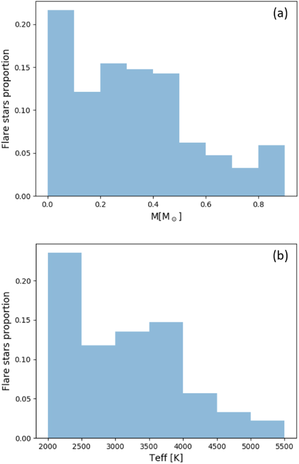
In this study, the K2 light curves of 3501 M dwarfs and 7249 K dwarfs have been analyzed. We detected flare events on 548 M-type (≈15.62%) and 343 K-type stars (≈4.73%). On the other hand, Shibayama et al. (2013) have found only 279 flaring G dwarfs in 80,000 solar-type stars (≈0.34%). We have investigated the proportion of flare stars in several specific temperatures and mass ranges (see Figure 16). Since we cannot verify which 80,000 solar-type stars Shibayama et al. (2013) investigated, we only show the M- and K-type flaring stars-to-all stars ratio in Figure 12. In general, the lower mass or cooler stars tend to have high flare occurrence probability. However, we found that the proportion of flare stars do not decrease with increasing temperatures or mass all along. A plateau appears in the temperature range of 2500–4000 K, or in the mass range of 0.1–0.3 M⊙. This means that stars with mass and temperature around 0.08–0.1 M⊙ and 2300–2500 K, respectively, have the highest proportion of flaring stars.

Figure 12. Panel (a) shows the number distribution of flaring stars-to-all stars ratio in mass, and panel (b) shows the same things in temperature. As a whole, the proportion of the flare stars decreases with increasing mass or temperature. However, there is a plateau in the range of 0.08–0.3 M⊙ or 2000–4000 K, respectively.
Download figure:
Standard image High-resolution image4.2. Flare Amplitudes and Energies
The flare peak amplitude, , can be used to classify the flares in different levels. In general, the flares with are called the hyperflares (Chang et al. 2018) with the corresponding flare peak flux reaching more than 100% stellar luminosity. We found 19 hyper-flare events in 15 M dwarfs (Table 1).


Table 1. 19 Hyperflares on 15 M Dwarfs
| EPIC | Eflare | Duration | Tpositiona | Teff | Mass | |
|---|---|---|---|---|---|---|
| (Log(erg)) | (hr) | (JD-2454833) | (K) | (M⊙) | ||
| 211441334 | 12.11 | 34.86 | 2.0 | 2334.23 | 3384 | 0.147 |
| 210715010 | 5.33 | 32.92 | 2.0 | 2273.14 | 2376 | 0.082 |
| 211441334 | 3.64 | 34.86 | 2.5 | 2334.26 | 3384 | 0.147 |
| 206181579 | 2.74 | 33.68 | 2.0 | 2153.05 | 2991 | 0.121 |
| 210843552 | 2.64 | 35.08 | 2.0 | 2259.02 | 3711 | 0.378 |
| 210626041 | 2.26 | 35.11 | 2.9 | 2268.34 | 3724 | 0.376 |
| 211441334 | 2.12 | 34.10 | 2.0 | 2319.28 | 3384 | 0.147 |
| 211796220 | 1.88 | 33.64 | 2.0 | 2316.15 | 3037 | 0.121 |
| 201396752 | 1.87 | 33.50 | 2.0 | 2019.88 | 2981 | 0.120 |
| 210658027 | 1.60 | 34.55 | 2.5 | 2237.03 | 3572 | 0.284 |
| 211577353 | 1.47 | 34.19 | 2.5 | 2323.00 | 3458 | 0.200 |
| 211107439 | 1.44 | 34.91 | 4.4 | 2297.47 | 3611 | 0.289 |
| 211016654 | 1.37 | 34.85 | 2.9 | 2232.89 | 3622 | 0.270 |
| 210450012 | 1.37 | 34.06 | 2.0 | 2241.14 | 3375 | 0.196 |
| 201396752 | 1.32 | 33.32 | 2.0 | 1989.40 | 2981 | 0.120 |
| 210395925 | 1.27 | 34.26 | 2.0 | 2268.03 | 3512 | 0.214 |
| 210454684 | 1.24 | 34.56 | 2.9 | 2233.87 | 3597 | 0.292 |
| 211107439 | 1.15 | 34.88 | 3.9 | 2297.49 | 3611 | 0.289 |
| 211091536 | 1.10 | 34.18 | 2.0 | 2271.14 | 3446 | 0.196 |

Note.
aThe flare time position in units of Julian day-2454833 day in the light curve.Download table as: ASCIITypeset image
A flare with was detected on the M dwarf EPIC 211441334 (Figure 13). This flare released an energy of about 7 × 1034 erg. EPIC 249394096 produced the maximum flare of K-type stars with a peak flare amplitude of about 0.78 (78%) and an energy ≈2 × 1035 erg (see Figure 14). From the work of Shibayama et al. (2013), the maximum of G-type stars can be found to be about 0.32 (32%) with an energy ≈3 × 1035 erg on KIC 12354328. No hyper-flare event has been discovered in K- or G- type stars. The reason is that the value is based on the luminosity baseline of the stars. Because the K- and G- type stars are brighter than the M dwarfs, the of the flares with the same energy on stars of K- and G-type would be smaller than those of M-type stars. Figure 15 provides a summary of the correlations between the value and the stellar temperature or the mass. We found the power-law expressions: and . Namely, a negative correlation. However, the correlations with the flare energy and the stellar parameters are positive, and the power-law expressions are and Eflare ∝ M2.43. Note that Figures 8 and 9 also show that the later type dwarfs tend to have higher but smaller flare energies, and the earlier type dwarfs tend to have the lower but larger flare energies. Some of the most powerful flares in M dwarfs can reach the same order as the powerful flares in G-type dwarfs, which are hotter than the M dwarfs.


Figure 13. Light curve of the M dwarf EPIC 211441334 which has the highest flare (upper panel). The rotation period of EPIC 211441334 is 2.8 days. The other stellar parameters are M ≈ 0.147 M⊙, and Teff ≈ 3384 K. We detected two hyper-flare events on this star. One flare with released an energy Eflare ≈ 1 × 1034 erg in about 2.5 hr (a), the other and the most powerful flare with released an energy Eflare ≈ 7 × 1034 erg in about 3 hr (b).


Download figure:
Standard image High-resolution image
Figure 14. Description of the highest flares of K-type we detected. The upper panel shows the light curve of the K dwarf EPIC 249394096 with M ≈ 0.532 M⊙, Teff ≈ 3989 K, and P ≈ 0.35 d. Panel (a) shows the flare with the highest value (≈0.78) of K dwarfs. This flare released an energy Eflare ≈ 2 × 1035 erg in about 4 hr. Panel (b) shows the other flare, , which released an energy Eflare ≈ 1 × 1034 erg in about 1.5 hr.


Download figure:
Standard image High-resolution image
Figure 15. Panels (a) and (b) show the negative correlations between of different stars with the stellar parameters (temperature in panel (a); mass in panel (b)). The correlations between the flare energy and similar stellar parameters shown in panels (c) and (d), however, are positive.

Download figure:
Standard image High-resolution image4.3. Flare Activities, Rotation Periods, and Stellar Ages
The rotation period of a star is known to be related to the stellar age, and younger stars show more rapid rotation according to the gyrochronology relation (Skumanish 1972; Barnes 2003, 2007, 2010; Reinhold & Gizon 2015). Angus et al. (2015) correlated the rotation period measurements of 310 Kepler stars with asteroseismic ages, six field stars including the Sun and stars in the Hyades and Coma clusters with precise age determination to calibrate the gyrochronology relation. These authors confirmed the general trend for a power-law approximation with rotation period, P, increasing from about 7 days at t(age) ∼0.5 Gyr to about 20–40 days at t ∼ 10 Gyr (see Figure 6 in their paper), while cautioning the presence of deviations from the precise relation and the need for further investigations.
Since the discovery of the superflares by Maehara et al. (2012), the relationship between the superflare frequencies/magnetic activities and the rotation periods and hence the stellar age, by implication, has been investigated by Wu et al. (2015), Karoff et al. (2016), Chang et al. (2017, 2018), Maehara et al. (2017), Notsu et al. (2017), and He et al. (2018). Briefly speaking, from a statistical study of the chromospheric emissions of 5648 solar-type stars including 48 superflare stars culled from the Kepler data, Karoff et al. (2016) showed that the superflare stars have a larger S-index, which is a measure of the Ca ii and K line emission level. Wu et al. (2015) and Chang et al. (2017, 2018) examined the link between stellar rotation periods and superflare frequencies of different types of low-mass stars and showed that P = 10 days is likely to be a critical value dividing active and inactive stars. Maehara et al. (2017) compared the size frequency distributions of the star spots with the flare frequencies of the solar-type stars in detail. They found that generally not just the flare occurrence rates but also the spot sizes tend to decrease if the stellar rotation periods increase. Note that He et al. (2018) found that there exists no clear correlation between the timing of the flare occurrence and the locations of the magnetically active regions identified by the star spots according to their detailed analysis of the light curves of three solar-type stars (KIC 6034120, KIC 311833, and KIC 10528093). This result is in general agreement with the work of Hou (2018). Using high-resolution spectroscopic measurements with Subaru, Notsu et al. (2017) compared the superflare frequencies of some solar-type stars with their corresponding X-ray fluxes and the Li abundance, which can be used as a proxy of the stellar ages. They found that young stars tend to be fast-rotating and magnetically active even though some old and slowly rotating stars as old as the Sun can also produce superflares.
Following these recent studies, it is possible to explore the dependence of flare activity with the stellar age making use of the gyrochronology relation mentioned earlier. With the gyrochronology formulation published by Barnes (2007), we found old flaring stars (see Table 2), and three flaring solar-type stars (KIC 6633602, KIC 8212826, and KIC 11401109) are older than the Sun. The oldest one, KIC 11401109, is up to 6 Gyr old. However, the oldest M- (∼2.8 Gyr) and K-type (∼2.9 Gyr) flaring stars with P > 40 days are younger than the Sun.
Table 2. Old and Slow-rotating Flaring Stars
| Star | Teff | Mass | log(g) | P | B − V | Agea | δAgea |
|---|---|---|---|---|---|---|---|
| (K) | (M⊙) | (days) | (Myr) | (Myr) | |||
| Sun | 5778 | 1.000 | 4.4 | 26.09b | 0.642c | 4565 | 766 |
| KIC 6504503d | 5499 | 0.902 | 4.6 | 30.5 | 0.742 | 4132 | 655 |
| KIC 6633602d | 5440 | 0.771 | 4.7 | 36.9 | 0.733 | 6152 | 1019 |
| KIC 8212826d | 6090 | 0.851 | 4.2 | 26.3 | 0.599 | 5815 | 1033 |
| KIC 9944137d | 5994 | 1.045 | 4.6 | 25.3 | 0.655 | 4049 | 666 |
| KIC 10736615d | 5690 | 0.922 | 4.6 | 30.8 | 0.750 | 4099 | 648 |
| KIC 11241343d | 5482 | 0.837 | 4.1 | 30.2 | 0.710 | 4543 | 735 |
| KIC 11401109d | 6025 | 1.058 | 4.5 | 29.1 | 0.623 | 6194 | 1083 |
| EPIC 211486352 | 3436 | 0.203 | 5.0 | 41.1 | 1.184 | 2808 | 413 |
| EPIC 201659529 | 3644 | 0.278 | 5.0 | 45.5 | 1.354 | 2726 | 402 |
| EPIC 211411789 | 3595 | 0.321 | 5.0 | 41.1 | 1.441 | 2027 | 289 |
| EPIC 246152729 | 4720 | 0.781 | 4.6 | 47.9 | 1.378 | 2915 | 434 |
Notes.
aBy using the Gyrochronology formulation from Barnes (2007). bMean solar rotation period from Donahue et al. (1996). cFrom Holmberg et al. (2006). dThe flaring solar-type stars from Shibayama et al. (2013).Download table as: ASCIITypeset image
We also found and Eflare increased with decreasing rotation period (see Figure 16). An obvious transition region appears at P ≈ 10 days in the M dwarfs' flare-period correlation. The level of flare activity drops sharply for those stars with rotation periods longer than 10 days. The undetectable transition region in the K and G dwarfs' flares may be due to observational bias. A possible reason is that higher stellar luminosities of K and G dwarfs will impede the identification of flares with small values in the K2 light curves, which are flux-limited. On the other hand, it is clear that fast-rotating stars exhibit more flare activities than stars with longer rotation periods.


Figure 16. Maximum (panel (a)–(c)) and Eflare (panel (d)–(f)) of each flare star vs. its rotation period. In general, the stars with the shorter rotation periods tend to have higher and Eflare. An obvious transition region appears at P ≈ 10 days in M dwarfs' flares that is not detectable in other spectral types.


Download figure:
Standard image High-resolution image4.4. Flare Durations
Figure 17 compares the flare energy variations with flare durations in M-, K-, and G-type dwarfs. Since we used the LC data whose time resolution is about 29.4 minutes and the flare detection algorithm is designed to exclude the flare shape signal without three consecutive data points, the minimum flare duration of the flares in this study is 1.5 hr. For the 3589 flares detected in M dwarfs, the flare energy increases with increasing flare duration, and there is a flare energy upper limit that is about 1035 erg. This trend can also be found in K dwarfs. That is, 1647 flares have been detected in K dwarfs with an energy upper limit ≈4 × 1035 erg. Wu et al. (2015) showed that the upper limit of G dwarf flare energy is about 2 × 1037 erg, but they did not consider the Kepler response function for the flare energy calculation. The flare that released an energy of about 2 × 1037 erg was from the star KIC 11551430 in Wu et al. (2015). With an effective temperature 5541 K, we recomputed the flare energy by considering the Kepler response function and obtained a value of 6 × 1036 erg instead. Shibayama et al. (2013) detected 1547 superflares on 279 G-type dwarfs. The energy upper limit was found to be about 1036 erg. As mentioned before, a superflare that exploded on the young M-dwarf binary system DG CVn released an energy of 4 ×1035–9 × 1035 erg larger than the M dwarfs' flare energy upper limit (∼1035 erg) we found (Osten et al. 2016). This means that the magnetic energy storage mechanism of the binary system may be capable of yielding more powerful flares than single stars.

Figure 17. Comparison of the flare energy variation and the flare duration. Panel (a) shows the distribution of 3589 flares of the M dwarfs; panel (b) for 1647 flares of the K dwarfs. The flares with longer duration have stronger energy released. The energy upper limits in M- and K-type dwarfs are about 1 × 1035 and 4 × 1035 erg, respectively. The G dwarf flare detected by Shibayama et al. (2013) is shown in panel (c), the lower limit of the flare energy increases with the flare duration, the energy upper limit is about 1036 erg.
Download figure:
Standard image High-resolution image4.5. Flare Occurrence Percentages
The stars with the top 10 highest flare occurrence percentages are shown in Table 3. Figure 18 shows the correlation of the flare occurrence percentages with the stellar masses and rotation periods. The stars are divided into several groups according to the rotation period. With similar rotation periods, the lower mass stars tend to be more active than the more massive stars. The flare occurrence percentage of stars is also significantly affected by the rotation period. For the four M dwarfs with rotation periods >40 days, their flare occurrence percentages are all below 0.5%, which is lower than some more massive stars with faster rotation periods. A transition region appears near 0.6–0.7 M⊙, forming a "hockey stick" pattern. The highest flare occurrence percentages in each rotation group are 3.22% (P ≤ 10 days); 1.84% (10 days < P ≤ 20 days); 1.98% (20 days < P ≤ 30 days); 0.95% (30 days < P ≤ 40 days); and 0.78% (P > 40 days).

Figure 18. Comparison of the flare occurrence percentage with the stellar mass. The stars have been classified by rotation period with a transition region appearing near 0.6–0.7 M⊙. The "hockey stick" pattern indicates that active stars usually have the lower mass and faster rotation period.
Download figure:
Standard image High-resolution imageTable 3. The Stars with the 10 Highest Flare Percentages
| EPIC | Flare Percentage (%) | Mass (M⊙) | Teff (K) | Prot (day) | Max | Max Eflare[Log(erg)] |
|---|---|---|---|---|---|---|
| 210564347 | 3.23 | 0.223 | 3496 | 5.121 | 0.065 | 33.19 |
| 206262336 | 2.72 | 0.222 | 3495 | 9.741 | 0.185 | 33.59 |
| 210909746 | 2.45 | 0.373 | 3748 | 4.039 | 0.439 | 34.50 |
| 206024567 | 2.39 | 0.278 | 3585 | 6.052 | 0.234 | 33.75 |
| 210434976 | 2.33 | 0.509 | 3954 | 2.553 | 0.215 | 34.48 |
| 211120664 | 2.32 | 0.320 | 3683 | 1.497 | 0.199 | 33.92 |
| 211006108 | 2.30 | 0.268 | 3582 | 0.959 | 0.470 | 34.34 |
| 201738857 | 2.16 | 0.206 | 3463 | 1.378 | 0.092 | 33.17 |
| 211724534 | 2.16 | 0.282 | 3604 | 2.454 | 0.141 | 33.72 |
| 206050032 | 2.07 | 0.090 | 2617 | 1.244 | 0.095 | 31.68 |

Download table as: ASCIITypeset image
4.6. Flare Frequency Distributions
In a previous study, the solar and stellar flare activities have been interpreted in terms of a magnetic reconnection-driven, self-organized critical system (Boffetta et al. 1999). The corresponding solar/stellar flare frequency distribution FFD can be expressed as the power law:

We estimate the cumulative FFDs and derive the power-law index by using the maximum likelihood method (Clauset et al. 2009; Klaus et al. 2011) with a Python package "powerlaw" which is a toolbox for analysis of heavy-tailed distributions (Alstott et al. 2014). Figure 19 shows the cumulative FFDs of M, K, and G dwarfs. The power-law indices of M and K dwarfs are γ = 1.82 ± 0.02, γ = 1.86 ± 0.02, respectively, and these are quite close to each other. Shibayama et al. (2013) showed that the power-law index of G-type stars is γ ≈ 2.2 by binning the data set while our result is γ = 2.01 ± 0.03. The flare occurrence rate of M dwarfs is about once in 0.6 yr for Eflare > 1 × 1033 erg and once in 6.5 yr and 350 yr for superflares with Eflare of 1034 erg and 1035 erg, respectively. In comparison, the K dwarfs' flare occurrence rate is about once in 4.7 yr with Eflare > 1 × 1034 erg, namely, more frequent than the M dwarfs'. The G dwarfs' flare occurrence rate of the flares with Eflare > 1 × 1035 erg is also higher than the M dwarfs', it is about once in 320 yr. For the solar-like stars (5600 K ≤ Teff < 6000 K and Prot > 10 days and log(g) > 4), the flare occurrence rates are about once in 800 yr with Eflare > 1 × 1034 erg and once in 5000 yr with Eflare > 1 ×1035 erg (Shibayama et al. 2013). If we only consider the flares from stars with rotation periods shorter than 10 days, the power-law indices of M- and K-type stars (1.78 versus 1.82) are nearly the same (see Figure 20), it may indicate they have similar flare generation mechanisms.

Figure 19. Panels (a), (b), and (c) show the cumulative FFDs of the M-type, K-type, and G-type stars, respectively. The data of the G dwarfs' FFD are from Shibayama et al. (2013).
Download figure:
Standard image High-resolution image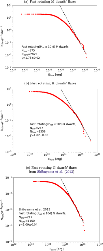
Figure 20. Panels (a), (b), and (c) show the FFD of the fast-rotating M-type, K-type, and G-type stars that have P ≤ 10 days, respectively. The data of the G dwarfs FFD are from Shibayama et al. (2013).
Download figure:
Standard image High-resolution image5. Summary
In order to examine the different levels of influence on the habitability of exoplanets orbiting around the low-mass stars of different spectral types and to bridge the K-dwarf gap of previous studies, we present a comparative study of the magnetic activities of low-mass stars from M type to G type. We analyzed M and K dwarfs' K2 LC data and compared the flares we found on M and K dwarfs with the G dwarfs' flares from Shibayama et al. (2013). The samples we collected in this study are 3501 M dwarfs within 100 pc and 7249 K dwarfs within 200 pc from the Earth. With our flare detection algorithm and investigation, we have detected 3589 flares on 548 M dwarfs, and 1647 flares on 343 K dwarfs. The flare peak amplitude, decreases with increasing mass and effective temperature of the stars; the flare energy, Eflare, however, varies in an opposite manner. The durations of most of the flares we detected are 1.5 hr according to our flare detection method, and the number of the flares with longer duration is fewer than of the flares with shorter duration. The longest duration of a flare we found here is about 5 hr. The longer the duration of the flare is, the stronger explosive energy may be, but there is an energy upper limit. The energy upper limits of M, K, and G dwarfs are 1035 erg, 4 × 1035 erg, and 1036 erg, respectively. We computed the rotation periods of 548 M-type and 343 K-type flaring stars by using the Lomb–Scagle method with Python package gatspy (VanderPlas & Ivezic 2015), which should be as good as AutoACF (McQuillan et al. 2014). Most of the magnetically active M-, K-, and G-type dwarfs have rotation periods in the range of 0.1 to 10 days. By using the Gyrochronology formulism (Barnes 2007; Angus et al. 2015), we found that some flaring solar-type stars could be older than the Sun. We estimated the flare percentages of all flaring stars. We found that stars with smaller mass and faster rotation period (P ≤ 10 days) are usually more active. A transition region appears near 0.6–0.7 M⊙, the stars with the mass larger than this range would be much less magnetically active. We calculated the cumulative FFDs power-law index (γ) by using the maximum likelihood method, and γ of M, K, and G dwarfs are 1.82 ± 0.02, 1.86 ± 0.02, and 2.01 ± 0.03, respectively. In addition, we estimated the cumulative frequencies of the flares on fast-rotating stars with P ≤ 10 days of every spectral type, γ = 1.78 ± 0.02 (M dwarfs), γ = 1.82 ± 0.03 (K dwarfs), γ = 2.09 ± 0.04 (G dwarfs). The cumulative FFDs power-law indices of all or fast-rotating M and K types stars are nearly the same.

We thank the reviewer for useful comment and suggestions. This research was supported in part by grant No. 107-2119-M-008-012 of MOST, Taiwan, and grant No. 119/2017/A3 of FCDT of Macau, MSAR.
Software: powerlaw (Alstott et al. 2014), gatspy (VanderPlas & Ivezic 2015).
: Appendix
Because of the shorter time coverage of the K2 observations, i.e., only three months (∼80 days), in comparison to the full three-year data coverage in the prime mission, there is a question regarding to what extent the rotation period determination can be considered reliable. Before addressing this issue, we need to first show that the Lomb–Scargle method used in the present study is a good technique.
McQuillan et al. (2014) calculated 34,030 dwarfs' rotation periods by using an automated version of the Autocorrelation function (AutoACF). To test our method, we randomly selected 1000 targets in McQuillan et al. (2014) and estimated their rotation periods with the same length of time series (Q3–Q14, ≈three years) of the LC data by using the Lomb–Scargle method and compared our results with those of McQuillan et al. (2014). We found three linear correlation groups and the fractions are 739/1000 (group 1:1), 227/1000 (group 1:2), 12/1000 (group 1:3), and 22 stars in the "no" groups (see Figure 21). The stars in the group 1:2 usually have active regions on their opposite hemispheres, it is hard to identify whose results are correct by visual checking. On the other hand, after visual checking the light curves and phase curves of stars in the group 1:3 and the no groups, were confident that our results are more precise than those of McQuillan et al. (2014) for most of the stars (see Figure 22 and Table 4). Consequently, the rotation period estimation method and the Python package gatspy (VanderPlas & Ivezic 2015) used in the present analysis are reliable.

Figure 21. Direct comparison between rotation periods of the random 1000 targets in McQuillan et al. (2014) with our estimates by using the Lomb–Scargle and that of McQuillan et al. (2014) by using AutoACF. Three correlation groups are marked in dashed lines with different colors, 1:1 (red), 1:2 (blue), 1:3 (green), and the fractions are 739/1000 (group 1:1), 227/1000 (group 1:2), 12/1000 (group 1:3), and 22 stars in the "no" group.
Download figure:
Standard image High-resolution image
Figure 22. Comparison of the rotation period results of KIC 4243104 (upper panel) and KIC 391772 (lower panel), respectively, given in McQuillan et al. (2014) with those determined by using the Lomb–Scargle method as used in this study. From left to right, the Kepler light curves from Q3 to Q14, the phase curves from McQuillan et al. (2014), and the phase curves from the present work. Note that KIC 4243104 belongs to the 1:3 groop, and KIC 391772 is in the "no" groups.
Download figure:
Standard image High-resolution imageTable 4. A Comparison of Rotation Period Results of McQuillan et al. (2014) (Pmcq) and This Study (P) for 34 Stars in the Group 1:3 and the "No" Group
| KIC | Group | Pmcq | P | Better |
|---|---|---|---|---|
| (days) | (days) | |||
| 2835051 | No | 39.835 | 16.766 | uncertain |
| 3101129 | No | 27.394 | 23.991 | no |
| 3102749 | No | 8.163 | 9.078 | yes |
| 3339107 | No | 48.654 | 43.946 | yes |
| 3357261 | No | 39.139 | 43.714 | no |
| 3658166 | 1:3 | 45.337 | 15.718 | yes |
| 3727538 | 1:3 | 37.868 | 12.877 | yes |
| 3839850 | 1:3 | 43.062 | 13.796 | no |
| 3971772 | No | 36.964 | 1.540 | yes |
| 4068018 | 1:3 | 39.506 | 13.268 | yes |
| 4078087 | No | 30.197 | 17.174 | no |
| 4135605 | 1:3 | 39.611 | 12.628 | yes |
| 4143604 | No | 41.719 | 17.574 | uncertain |
| 4147960 | No | 27.832 | 39.151 | no |
| 4160250 | No | 16.235 | 18.064 | yes |
| 4164424 | No | 39.993 | 23.198 | no |
| 4243104 | 1:3 | 43.779 | 15.061 | yes |
| 4349935 | No | 34.313 | 19.260 | yes |
| 4474200 | 1:3 | 37.053 | 12.433 | yes |
| 4576715 | No | 41.032 | 47.109 | yes |
| 4579434 | No | 43.682 | 16.532 | yes |
| 4641447 | No | 42.352 | 47.545 | yes |
| 4737595 | No | 22.173 | 2.276 | no |
| 4852379 | No | 38.464 | 16.726 | yes |
| 4930560 | No | 10.367 | 89.681 | no |
| 5006728 | 1:3 | 43.302 | 14.561 | yes |
| 5020113 | 1:3 | 49.396 | 17.953 | yes |
| 5027511 | No | 43.511 | 35.645 | no |
| 5093851 | No | 14.637 | 16.550 | yes |
| 5094486 | 1:3 | 38.017 | 13.040 | yes |
| 5124568 | 1:3 | 40.755 | 13.626 | yes |
| 5181086 | No | 42.390 | 16.368 | yes |
| 5191975 | 1:3 | 35.630 | 12.112 | yes |
| 5195911 | No | 43.769 | 16.270 | yes |
Note. We visually checked the light curves and phase curves of these stars to determine which results are better. The column "better" shows that we obtain better results by using the Lomb–Scargle method from Python package gatspy (VanderPlas & Ivezic 2015).
Download table as: ASCIITypeset image
Figure 23 shows another example, EPIC 246152729, which is one of our targets, and we found a possible rotation period of 47.85 days in the K2 80 days data set. Because the length of the K2 time series data is not as long as the Kepler (prime mission) data, it affects the ability to detect the rotation period of stars with a long-term brightness variation. Figure 24 displays the light curves, periodograms, and phase curves of Q3–Q14 and each quarter of KIC 2570277 with a long rotation period in group 1:1 as the examples. The period obtained from 3 yr data is ≈44.085 days, but only two quarters (Q6 and Q7) have similar results. The periods derived from the other quarters are significantly different from the correct value. It demonstrates that the stars with long periods up to 50 days could be identified in the data with the timescales of about three months, but the results may not be correct if the light curves are irregular.

Figure 23. Left panel shows the light curve of EPIC 246152729 in the timescales of about 80 days. The middle panel and right panel show the periodogram and phase curve of EPIC 246152729, respectively. Its rotation period is 47.85 days.
Download figure:
Standard image High-resolution image
Download figure:
Standard image High-resolution image
Download figure:
Standard image High-resolution image
Figure 24. Light curves, periodograms, and phase curves of Q3–Q14 and each quarter of KIC 2570277 with a long rotation period in group 1:1. The period obtained from 3 yr data is ≈44.085 days, but only two quarters (Q6 and Q7) have similar results. This demonstrates that the results of the stars with long periods up to 50 days derived from the data with the timescales of about three months may not be correct.
Download figure:
Standard image High-resolution image
We calculated the percentages of the correct period of the period ranges in individual quarters. We considered the stars in group 1:1 (739 stars) only. It is clear that in three month data sets, the shorter the rotation period is, the higher the confidence level would be for getting the precise period results (Table 5). The accuracy rates are 92.54% ± 2.00% (P ≤ 10 days), 78.46% ± 2.24% (10 days < P ≤ 20 days), 50.50% ± 4.88% (20 days < P ≤ 30 days), 33.78% ± 4.79% (30 days < P ≤ 40 days), and 33.22% ± 8.02% (40 days < P ≤ 50 days).
Table 5. Accuracy Rates of Different Period Intervals in Each Quarter Data
| Quarter | TLa | P(<10) | P(10–20) | P(20–30) | P(30–40) | P(40–50) |
|---|---|---|---|---|---|---|
| (days) | (%) | (%) | (%) | (%) | (%) | |
| Q3 | 89.27 | 88.406 | 76.703 | 54.545 | 42.857 | 50.000 |
| Q4 | 89.83 | 89.286 | 77.741 | 56.150 | 33.654 | 41.176 |
| Q5 | 94.67 | 95.062 | 79.725 | 54.396 | 42.157 | 35.417 |
| Q6 | 89.85 | 88.889 | 77.027 | 44.118 | 31.250 | 43.590 |
| Q7 | 89.37 | 92.857 | 77.741 | 56.383 | 34.286 | 47.059 |
| Q8 | 66.98 | 89.286 | 70.100 | 34.043 | 21.154 | 5.882 |
| Q9 | 97.41 | 98.765 | 81.787 | 55.495 | 40.196 | 29.167 |
| Q10 | 93.42 | 95.238 | 82.432 | 44.853 | 21.250 | 33.333 |
| Q11 | 97.12 | 94.048 | 79.734 | 56.383 | 42.857 | 31.373 |
| Q12 | 82.61 | 94.048 | 77.741 | 40.957 | 33.654 | 21.569 |
| Q13 | 90.32 | 92.593 | 76.976 | 50.549 | 33.333 | 39.583 |
| Q14 | 97.18 | 92.063 | 83.784 | 58.088 | 28.750 | 20.513 |
| Average | 89.84 | 92.545 | 78.458 | 50.497 | 33.783 | 33.221 |
Note.
aTime length of the Quarter.Download table as: ASCIITypeset image