


Abstract
A test-particle model describing the energization of electrons in a turbulent plasma is presented. Parameters are chosen to represent turbulence in a magnetic structure of the solar corona. A fluctuating electric field component parallel to the background magnetic field, with properties similar to those of Kinetic Alfvén Waves, is assumed to be present at scales of the order of the proton Larmor radius. Electrons are stochastically accelerated by multiple interactions with such fluctuations, reaching energies of the order of 102 eV within tens to hundreds of seconds, depending on the turbulence amplitude. For values of the large-scale plasma velocity fluctuation of the order of tens of kilometers per second, the power absorbed by electrons per surface unit is of the order of that typically necessary to heat the corona. The power that electrons absorb from fluctuations is proportional to the third power of the large-scale velocity amplitude, and is comparable with the power associated with the turbulent cascade. Therefore, this mechanism can be considered as an equivalent kinetic dissipation for turbulence, and it can play a relevant role in the heating of electrons in the corona.
Export citation and abstract BibTeX RIS
1. Introduction
The problem of heating of the solar corona has received considerable attention in the literature. It is now widely accepted that the source of the high temperature observed in the outer atmosphere of the Sun lies in the photospheric motions moving and shuffling magnetic field lines, which extend from the photosphere up to the Corona. Models have been proposed where this mechanism would transfer magnetic and kinetic energy from low atmospheric layers up to the magnetized Corona, both through quasi-stationary magnetic field deformations (e.g., Parker 1972, 1988), or by higher frequency waves propagating along the magnetic field (e.g., Lee & Roberts 1986; Hollweg 1987; Malara et al. 1996; Milano et al. 1997). Observational evidence has recently been found for the presence of torsional motions in magnetic elements of the chromosphere (Srivastava et al. 2017), as well as of Alfvén waves in the corona (Tomczyk & McIntosh 2009).
The coronal heating problem and the typical description of turbulent flows have many points in common. In fact, energy injection at large spatial scales due to photospheric motions, the subsequent nonlinear cascade of energy, and the final dissipation at small scales are the main features characterizing turbulent flows. This idea has led to the formulation of models of coronal heating based on turbulence, where magnetohydrodynamic (MHD) or reduced MHD (Strauss 1976) direct numerical simulations are employed (Einaudi et al. 1996; Hendrix & Van Hoven 1996; Dmitruk & Gomez 1997, 1999; Dmitruk et al. 1998; Rappazzo et al. 2008; Rappazzo & Velli 2011; van Ballegooijen et al. 2011; Dahlburg et al. 2012, 2016). Further theoretical contributions have been provided by "reduced" approaches to MHD turbulence, based on the shell-model technique (Giuliani & Carbone 1998; Boffetta et al. 1999), that have allowed us to describe extended spectra with a limited computational effort (Nigro et al. 2004, 2005; Buchlin & Velli 2007; Verdini et al. 2012; Cadavid et al. 2014). Due to the strong axial magnetic field B0, such models predict transverse velocity and magnetic field fluctuations that propagate along B0 at the Alfvén velocity, while nonlinear effects produce an energy cascade developing in the directions perpendicular to B0. Another point in favor of the "turbulent" scenario is that in turbulent magnetofluids dissipation takes place via a large number of small dissipative events, whose statistics are determined by the properties of intermittency (e.g., Frisch 1995; Sorriso-Valvo et al. 1999). In the turbulent corona, these events should be revealed as microflares or nanoflares. In fact, the statistical properties of flares (Lin et al. 1984; Crosby et al. 1993; Krucker & Benz 1998; Parnell & Jupp 2000) display features such as distribution of energy, peak power, duration, and waiting times that are compatible with those of dissipative events in turbulence (Boffetta et al. 1999; Lepreti et al. 2001).
Though the dynamics of turbulence in MHD has been deeply investigated, mechanisms that are responsible for energy dissipation in low-collisional plasmas are still poorly understood. In particular, in the coronal plasma collisional dissipative coefficients have values so low that collisional dissipative lengths turn out to be smaller than scales where dispersive and kinetic effects become relevant. Therefore, it can be inferred that kinetic effects can play an important role in the smallest-scale part of the turbulence spectrum, and they can be (at least partially) responsible for transferring energy from fluctuations to particles, thus contributing to energize the plasma. The kinetic scenario is more complex than in MHD; for instance, in corona the various ion species and electrons can all have different temperatures. In the present paper, we want to address this point by studying the stochastic interaction between electrons and fluctuations at scales comparable with the proton Larmor radius Rp, in order to assess whether such interaction can be considered as an eligible mechanism for the electron heating.
In the presence of a strong background magnetic field B0, the energy cascade preferentially takes place perpendicularly to B0 (e.g., Shebalin et al. 1983; Carbone & Veltri 1990; Oughton et al. 1994). Then, it is expected that at smaller scales the fluctuation energy tends to concentrate in nearly perpendicular wave vectors. This idea is supported by observational data showing that the distribution of wave vectors of magnetic fluctuations in the solar wind has a significant population quasi-perpendicular to the ambient magnetic field (Matthaeus et al. 1986, 1990). Dispersive MHD waves belonging to the Alfvén branch, with l∥ ≫ l⊥, at scales l⊥ ∼ Rp (l∥ and l⊥ being the wavelengths parallel and perpendicular to B0, respectively) are known as kinetic Alfvén waves (KAWs). The above considerations suggest that the coronal turbulence at scales l⊥ ∼ Rp is significantly composed by KAW-like fluctuations. An extensive analysis of KAW physics can be found in Hollweg (1999). Many solar wind observational analyses (Bale et al. 2005; Sahraoui et al. 2009; Podesta & Tenbarge 2012; Salem et al. 2012; Chen et al. 2013; Kiyani et al. 2013), theoretical works (Howes et al. 2008a; Sahraoui et al. 2009; Schekochihin et al. 2009), and numerical simulations (Gary & Nishimura 2004; Howes et al. 2008b; TenBarge & Howes 2012) have suggested that KAWs can play an important role in the dissipation of turbulent energy. The nature of the turbulent cascade has been investigated by high-resolution multispacecraft measurements (Narita et al. 2010), suggesting that fluctuations at ion scales can be highly oblique, consistent with KAW fluctuations (Sahraoui et al. 2010). Moreover, the generation of KAWs has been observed in simulations of Alfvén wave phase-mixing, a phenomenon that mimics nonlinear interactions in turbulence (Vàsconez et al. 2015; Pucci et al. 2016; Valentini et al. 2017), as well as in simulations of Alfvénic packets collisions (Pezzi et al. 2017a, 2017b, 2017c), while the nonlinear regime of wave-particle interaction in the case of KAWs fluctuations has been investigated in Vàsconez et al. (2014). A property of KAWs that is particularly relevant in such context is that they are endowed with a nonvanishing electric field component δE∥ parallel to the background magnetic field B0 (e.g., Hollweg 1999). In contrast, MHD theory, valid at large scales, predicts δE∥ = 0 for any fluctuation. Such a component can allow for an energy transfer from fluctuations to particles. For instance, Voitenko & Goossens (2004) studied the heating of several species of ions in the corona by KAWs using a test-particle approach.
In the present paper we describe a model for the stochastic energization of electrons in a turbulent plasma permeated by a strong axial magnetic field B0. The model, which employs a test-particle approach, assumes that fluctuations are essentially Alfvénic and, at scales of the order of Rp, characterized by quasi-perpendicular wave vectors and by a parallel electric field δE∥ with properties similar to those found in KAWs. At such scales the dynamics of electrons is simpler than that of ions because electrons are magnetized, i.e., they essentially move following magnetic field lines. This allows for a simplified treatment of the electron dynamics. In particular, the parallel electric field associated with small-scale fluctuations is responsible for electron acceleration. The model gives an estimate of the power P transferred from fluctuations to electrons. For values of the parameters typical of a coronal loop, such power favorably compares with that required to sustain the coronal high-temperature against radiative and conductive losses (Withbroe 1988). Moreover, the dependence of P on the fluctuation amplitude at large scales suggests that the energy transfer from fluctuations to particles can balance the spectral energy flux associated with turbulence (e.g., Frisch 1995), thus representing a possible kinetic mechanism for the turbulent dissipation. The plan is organized as follows: in Section 2 we describe the model with the underlying assumptions; in Section 3 the numerical results are described; in Section 4 we present a discussion of the results and draw conclusions; in the Appendix further details of the electron dynamics description are given.
2. The Model
In this section we describe and discuss the properties of the model and the underlying assumptions. We consider a simplified representation of a coronal loop, given by a magnetic structure with length L, characterized by a uniform background density n0 and a strong uniform background longitudinal magnetic field B0. The loop is perturbed by transverse motions, which generate velocity fluctuations at large transverse scales l⊥0. Such scales are assumed to correspond to those of photospheric motions. We indicate the amplitude of velocity fluctuations at large scales l⊥0 by δv⊥0 = δv⊥(l⊥ = l⊥0), (where l⊥ indicates a given perpendicular scale length). Numerical simulations (e.g., Nigro et al. 2004; van Ballegooijen et al. 2011) of a typical coronal loop in the reduced MHD (RMHD) description show that time-averaged transverse velocity fluctuations at large scales are of the order of a few tens of kilometers per second. These values are in agreement with velocity estimations from nonthermal line broadenings in Corona (Acton et al. 1981; Warren et al. 1997; Chae et al. 1998). The values chosen for the above parameters are the following: B0 = 102 G, n0 = 109 cm−3, and l⊥0 = 3 × 108 cm, while δv⊥0 varies in the range between δv⊥0 = 2 × 106 cm s−1 and δv⊥0 = 8 × 106 cm s−1. The proton Larmor radius is Rp = mpcvth,p/(eB0), where mp and e are the proton mass and charge, c is the speed of light, and vth,p = (κBTp/mp)1/2 is the proton thermal velocity, with Tp the proton temperature and κB the Boltzmann constant. Assuming Tp = 1.5 × 10⁶ K and the above value of B0, we derive Rp ≃ 12 cm.
2.1. Fluctuations and Turbulence
Nonlinear interactions among fluctuations at scales l⊥0 transfer their energy toward smaller scales through a turbulent cascade. This phenomenon generates a spectrum that extends from large scales down to small scales l⊥K ∼ Rp, where kinetic effects become relevant. In the presence of a strong background magnetic field B0, assuming that magnetic perturbations remain much smaller than B0 and are characterized by l⊥0 ≪ l∥0, then the RMHD description can be applied (Strauss 1976). The RMHD approximation has been commonly adopted in many models of turbulence in coronal structures (e.g., Nigro et al. 2004; Buchlin & Velli 2007; Rappazzo et al. 2008; Rappazzo & Velli 2011; van Ballegooijen et al. 2011). Within RMHD, velocity  and magnetic field
  perturbations are essentially transverse to B0, motions are noncompressive ∇⊥ ·
  ⊥ = 0, and perturbations propagate along
  at the Alfvén speed vA = B0/(4πn0mp)1/2, mp being the proton mass. These properties also characterize Alfvén waves in MHD. In RMHD, nonlinear effects produce an energy cascade mostly in the transverse directions, i.e., a spectrum of transverse scales l⊥ much smaller than longitudinal ones l∥ are generated in the resulting turbulence. On this basis, we assume that fluctuations at small scales are Alfvénic and are characterized by a parallel scale length l∥K ≫ l⊥K ∼ Rp. In particular, we assume that the amplitudes of velocity and magnetic field fluctuations at such scales are related by

Waves belonging to the Alfvén branch with wavevector k quasi-perpendicular to B0 and  are commonly indicated as KAWs. We will focus on the effects of the component δE∥ parallel to B0, nonvanishing in KAWs, on the dynamics of electrons. In coronal conditions, it can be written in the form (Voitenko & Goossens 2004):

In order to estimate the amplitude δE∥ at scales (l∥, l⊥) = (l∥K, l⊥K), we make the following considerations. Numerical results by Nigro et al. (2008) derived from an RMHD-based model show that the kinetic energy turbulence spectrum has a single spectral index α = −5/3 with respect to k⊥ in the whole inertial range of turbulence, corresponding to a Kolmogorov spectrum. Therefore, we assume that the amplitude of velocity fluctuations at small scales δv⊥K is given by

where l⊥K = 2πRp. Nigro et al. (2008) and Malara et al. (2010) have also shown that, at sufficiently small transverse scales, there is an equipartition between kinetic and magnetic energies in fluctuations, which is consistent with our assumption (1). In MHD turbulence with strong longitudinal magnetic field B0, the energy cascade in the parallel direction tends to be inhibited. This is consistent with the RMHD assumptions, under which nonlinear interactions turn out to be efficient only in the direction perpendicular to the main magnetic field. In this context, the so-called critical balance principle (Goldreich & Sridhar 1995) postulates a balance between linear wave periods and nonlinear turnover timescales: l∥/cA ∼ l⊥/δv⊥, where the velocity fluctuation follows the Kolmogorov spectrum. According to this description and using the relation (3), we assume that fluctuations at small scales are characterized by transverse l⊥K and longitudinal l∥K lengths, which are related by:

We notice that the critical balance relation ( ), the condition
  (derived from Kolmogorov spectrum and energy equipartition assumption), and Equation (2) imply that
  for
for  , i.e., δE∥ increases with increasing k⊥. Therefore, the main contribution to the parallel electric field comes from fluctuations at the smallest scale l⊥K. In particular, using Equations (2)–(4) we derive the following estimation for the amplitude of the parallel electric field associated with fluctuations at small scales:

Summarizing, in the present model we assume that the main contribution to the parallel electric field is due to fluctuations, or "packets," at scales l⊥ = l⊥K = 2π Rp and l∥ = l∥K (with l∥K given by Equation (4)), whose amplitude is given by the expression (5). Such packets, which propagate in the longitudinal direction at velocity ±vA, have a finite lifetime tL which corresponds to the nonlinear time calculated at the smallest scale l⊥K:

where we used the relation (3).
The jump of electric potential in the parallel direction across each of such packets is

Using the above values of parameters, we find δV ∼ 1 V, corresponding, for an electron, to a jump in potential energy δU = ±e δV ∼ ±1 eV. Such a value of  is much less than the electron thermal energy Eth in a ∼106 K corona, where Eth ∼ 102 eV. Nevertheless, we will show that multiple crossing through such small potential energy jumps are able to gradually increase the electron energy up to values comparable to or even larger than Eth.
As a final remark, we observe that in a fluid description of hydromagnetic turbulence the small-scale end of the inertial range corresponds to the dissipative scale l⊥D. Therefore, a necessary condition for our model to be consistent is given by l⊥D ≤ l⊥K = 2πRp. This condition prevents collisions from quenching kinetic effects. Here we check whether such a condition is actually satisfied in our model. The dissipative scale is determined by imposing that at l⊥ = l⊥D the dissipative time tD becomes of the order of the nonlinear time tnl. In a plasma with a resistivity η the dissipative time is given by  , while the nonlinear time is tnl(l⊥) ∼ l⊥/δv⊥ (l⊥). The condition tD(l⊥D) ∼ tnl(l⊥D), along with Equation (3), gives

The (collisional) resistivity η can be estimated as the Spitzer resistivity ηS. Assuming a temperature T0 = 1.5 × 10⁶ K, we obtain ηS = 1.3 × 10⁻¹⁶ s. Using the above values for δv⊥0 and l⊥0, the expression (8) gives a collisional dissipative length l⊥D ∼ 1 cm. The value of the kinetic scale length considered in the model is l⊥K = 2πRp ≃ 70 cm. Therefore, l⊥,D ≪ l⊥,min. This suggests that kinetic effects can play a significant role in the small-scale range of the turbulence spectrum and could give a relevant contribution to the actual dissipation of the turbulent cascade.
2.2. Dynamics of Electrons
Each electron within the plasma is subject both to the electric and to the magnetic force; of course, only the former FE = −e E can modify the kinetic energy of particles EK = meu2/2, me and u being the electron mass and velocity, respectively. At the scales considered in the model, the electric field can be calculated using the generalized Ohm's law:

where pe is the electron pressure. The electric field component E⊥ perpendicular to B is mainly determined by the first term in Equation (9)

The Larmor radius of electrons RL,e is much smaller than the scale l⊥K considered in the model. Therefore, at scales l⊥ ≥ l⊥K the electron motion can be represented as the motion of the guiding center plus the gyromotion around the guiding center. The electric field perpendicular component E⊥ contributes to the electron motion determining a drift velocity ud = c E × B/B2 that coincides with the perpendicular component v⊥ of the macroscopic fluid velocity:

where we used Equation (10). Expression (11) also applies to ions, thus indicating that the perpendicular component of the fluid velocity can be interpreted as a kinetic drift motion. The corresponding electron kinetic energy is ![${E}_{K,d}={m}_{e}{{\boldsymbol{u}}}_{d}^{2}/2\,\simeq {m}_{e}{\left[\delta {v}_{\perp }({l}_{\perp 0})\right]}^{2}/2$](https://content.cld.iop.org/journals/0004-637X/871/1/66/revision1/apjaaf168ieqn12.gif) . Using the value δv⊥(l⊥0) = 5 × 106 cm s−1 we obtain an electron drift kinetic energy EK, d ≃ 7 × 10⁻³ eV. This is several orders of magnitude smaller than the electron thermal energy, which is of the order of 102 eV for temperatures of the order of 106 K. We conclude that the perpendicular electric field component E⊥ does not contribute to energize electrons. As a consequence, in order to investigate possible electron energization, we are led to consider the effects of the parallel electric field component.
. Using the value δv⊥(l⊥0) = 5 × 106 cm s−1 we obtain an electron drift kinetic energy EK, d ≃ 7 × 10⁻³ eV. This is several orders of magnitude smaller than the electron thermal energy, which is of the order of 102 eV for temperatures of the order of 106 K. We conclude that the perpendicular electric field component E⊥ does not contribute to energize electrons. As a consequence, in order to investigate possible electron energization, we are led to consider the effects of the parallel electric field component.
Let us consider a local reference frame, indicated by G', which moves with the local drift velocity ud ≃ v⊥, while we indicate by G a global inertial reference frame. The drift velocity ud significantly varies only at large spatial scales. Therefore, when describing the interaction between an electron and a fluctuation at small scales (l∥, l⊥) = (l∥K, l⊥K), we can neglect variations of ud across the fluctuation, i.e., we can use a single reference frame G' to describe the whole interaction. We also notice that, during a single interaction between an electron and a small-scale fluctuation, G' can be considered to be a quasi-inertial reference frame. To prove this we consider the typical timescale τ0 = l⊥0/δv⊥0 of variation for ud ≃ v⊥, and the electron crossing time τcross = l∥K/u∥ of a small-scale fluctuation. Using Equation (4) we find:

Being vA ≲ u∥ and l⊥K ≪ l⊥0 it follows that τcross ≪ τ0, i.e., the velocity ud of G' remains constant in time during the electron crossing. Therefore, to describe the interaction between an electron and a small-scale fluctuation in the reference frame G' we do not need to include any fictitious force in the electron equation of motion.
We observe the following: (i) being ud = v⊥, the small-scale fluctuation perceives the drift velocity ud as a (quasi-constant and uniform) bulk flow that advects the fluctuation itself in the direction perpendicular to B while the fluctuation is propagating along B at the Alfvén velocity. Therefore, in the reference frame G' the small-scale fluctuation only moves along B. (ii) The electric field in the reference frame G' is

Taking the transverse component of Equation (13) and using the definition of ud, we find that the transverse component of E' is vanishing:  , so that only the parallel component survives
  , the latter equality following from the transformation law (13).
ud being perpendicular to B, it follows that  , where
  and u∥ are the parallel components of the electron velocity with respect to G' and G, respectively. Therefore, the time evolution of the electron parallel velocity can be derived by solving the equation of motion in the reference frame G'. In conclusion, we will adopt the following description for the interaction between an electron and a small-scale fluctuation: in the quasi-inertial reference frame G' the electron moves along B and it is subject to the electric force
  while crossing a fluctuation at scales (l∥K, l⊥K). In the same reference frame G' the fluctuation also moves along B at a speed ±vA. Going back to the global reference frame G, we have only to add a perpendicular velocity component ud, which, however, is negligible with respect to u∥. Therefore, in order to describe the electron energization, the reference frames G and G' are essentially equivalent.
2.3. Modeling Electron Acceleration by Small-scale Fluctuations
We want to model in a simple way the effect of the parallel electric field associated with small-scale fluctuations on a population of test particles. On the basis of the above considerations, we assume that a given test-electron crosses a sequence of fluctuations in the direction parallel to the local magnetic field. We identify each electron by the index i = 1, ..., Ne, with Ne being the number of considered electrons, and we indicate by  the mth fluctuation crossed by the ith electron, with m = 1, ..., Mi, Mi being the number of fluctuations crossed by the ith electron during the whole calculation. In our model the electron interacts at any time only with a single fluctuation. Each time the ith electron comes out from a given fluctuation
  , it immediately enters the next fluctuation
  . We indicate by t0;i,m and t1;i,m the instants of time when the ith electron enters and exits from the fluctuation
  , respectively; as stated above, t1;i,m = t0;i,m+1. Moreover, u∥i = u∥i(t) is the parallel component of the ith electron velocity, and si,m = si,m(t) is the coordinate identifying the electron position in the parallel direction with respect to the fluctuation
  . In particular, the latter quantity is defined such that si,m(t = t0;i,m) = 0.
All fluctuations  have the same parallel length l∥K given by the expression (4) with l⊥K = 2πRp, and the same lifetime tL given by the Equation (6). The fluctuation
  moves along B with velocity σi,mvA, with σi,m = ±1. The sign σi,m of the propagation velocity is randomly chosen for each fluctuation. A parallel electric field with a given spatial profile along the longitudinal direction is associated with each fluctuation. We adopted the simplest choice of a spatially uniform parallel electric field profile across the fluctuation
  :
:
where ΔE∥i,m is the amplitude of the uniform electric field, which somehow represents the mean value of a more realistic nonuniform profile of the electric field. The quantity U∥i,m = u∥i − σi,mvA is the parallel velocity of the ith electron relative to the fluctuation  . For each fluctuation, the value of the amplitude ΔE∥i,m is chosen according to an assigned distribution. In particular, we considered two cases:
(1) a Gaussian distribution:

where the standard deviation δE∥K is the typical fluctuating electric field amplitude defined by Equation (5).
(2) a stretched-exponential distribution:
where Γ( · ) is the Euler function and β ≤ 2 is a parameter defining the shape of the distribution. For β = 2 the distribution (16) reduces to the Gaussian (15). Decreasing the value of β the tails of the distribution (16) become more and more relevant. The stretched-exponential distribution has been used to describe the distribution of fluctuation amplitudes at small scales in a turbulence with spatial intermittency (Frisch & Sornette 1997; Sorriso-Valvo et al. 2015, 2018). Indeed, intermittency corresponds to the presence at small scales of "extreme" fluctuations, whose amplitude is much larger than the rms value. In our model we used the value β = 1/2 in the expression (16) to simulate the presence of intermittency in the considered turbulence (Sorriso-Valvo et al. 2015). The profiles of the Gaussian and of the stretched-exponential distributions (with β = 1/2) are plotted in Figure 1. We will compare the results obtained with the two distributions (15) and (16), in order to check whether intermittency has an effect on the stochastic acceleration of test particles.
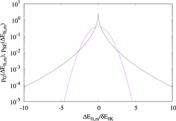
Figure 1. Gaussian distribution function pG (blue line) and stretched-exponential distribution function pSE with β = 1/2 (black line) are plotted in semilogarithmic scale, as functions of the parallel electric field amplitude ΔE∥i,m normalized to the standard deviation δE∥K.
Download figure:
Standard image High-resolution imageWhen the ith electron moves inside the fluctuation  , it is subject to a constant acceleration a∥i,m = −eΔE∥i,m/me, which can either increase or decrease the parallel velocity of the electron. Due to the constancy of a∥i,m, knowing the initial time t0;i,m, l∥K, and velocity u∥0;i,m = u∥(t0;i,m), it is a simple matter to calculate the final time t1;i,m and velocity u∥1;i,m = u∥(t1;i,m). The details of this calculation, as well as explicit expressions for t1;i,m and u∥1;i,m in the various cases, are given in the Appendix. In general, the electron can be either accelerated or decelerated, and, in the latter case, it is reflected back if u∥1;i,m and u∥0;i,m have opposite signs. We also take into account that each fluctuation has a finite lifetime tL (Equation (6)). If tL < (t1;i,m − t0;i,m) then the fluctuation disappears before the electron entirely crosses it; in this case, which can happen when the electron velocity is relatively low, the final time is set as t1;i,m = t0;i,m + tL and the final velocity is calculated accordingly. The final time and velocity are used as initial conditions for the interaction with the subsequent fluctuation
  : t0;i,m+1 = t1;i,m, u∥0;i,m + 1 = u∥1;i,m.
The described mechanism modifies only the parallel component u∥i,n of the electron velocity, while the perpendicular component  (in the reference frame G') due to the gyromotion remains unchanged. However, one can postulate some mechanism, like collisions or gradients of magnetic field intensity, which tends to isotropize the electron energy in the velocity space. For this reason we included in our model the possibility to transfer energy between parallel and perpendicular motion, so to obtain a complete isotropization. This is done by the following procedure: for m equal to a multiple of a given integer Miso the kinetic energy is calculated as
  . Then, the values of u∥i,m and
  are modified according to
 ![${u}_{\parallel i,m}={u}_{\perp i,m}^{{\prime} }={\left[2{E}_{\mathrm{kin}}^{{\prime} }/(3{m}_{e})\right]}^{1/2}$](https://content.cld.iop.org/journals/0004-637X/871/1/66/revision1/apjaaf168ieqn32.gif) . However, we found that the results of the model are robustly independent of the value chosen for Miso, i.e., the possible isotropization of the electron energy does not modify the considered acceleration mechanism.
. However, we found that the results of the model are robustly independent of the value chosen for Miso, i.e., the possible isotropization of the electron energy does not modify the considered acceleration mechanism.
The time evolution of each electron is initiated by setting t0;i,0 = 0 and  , where the sign of the initial velocity is randomly chosen, and the value
  corresponds to an initial kinetic energy
  , which is equal for all the test particles. The time evolution of particles is followed up to a final time tfin, which is chosen such that the average kinetic energy of the electron population reaches a value of a few hundreds of electronvolts. During the whole time evolution, each electron interacts with a large number Mi of fluctuations; typically Mi is of the order of 105. The sequence of the times t0;i,m (m = 0, ..., Mi) is distributed in the time interval
 ![$\left[0,{t}_{\mathrm{fin}}\right]$](https://content.cld.iop.org/journals/0004-637X/871/1/66/revision1/apjaaf168ieqn36.gif) , forming a dense (irregular) grid, which allows us to follow the detailed energy evolution of each test particle.
, forming a dense (irregular) grid, which allows us to follow the detailed energy evolution of each test particle.
3. Results
Figure 2 shows the time evolution of the energy  for four single particles when δv⊥0 = 4 × 106 cm s−1 and assuming the Gaussian distribution (15) for the electric field amplitudes. It can be seen that the time evolution of the particle energy is highly irregular: due to the large number of interactions with accelerating and decelerating fluctuations,
  increases and decreases on a short timescale. However, a closer inspection of Figure 2 reveals a general tendency for
  to increase. This can be more clearly seen by calculating the mean particle energy
  of a population formed by a large number Np of electrons. In particular, we used Np = 105 particles. In Figure 3 the mean kinetic energy is plotted as a function of time, for different values of the large-scale velocity fluctuation amplitude, ranging from δv⊥0 = 2 × 106 cm s−1 to δv⊥0 = 8 × 106 cm s−1.
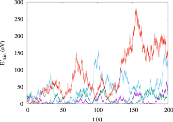
Figure 2. Single-particle kinetic energies  of four particles are plotted as functions of time, in the case δv⊥0 = 4 × 106 cm s−1 and a Gaussian distribution for ΔE∥i,k.
Download figure:
Standard image High-resolution image
Figure 3. Mean kinetic energy  of a population of Np = 105 particles plotted as functions of time, for various values of δv⊥0 ranging from 2 × 106 cm s−1 to 8 × 106 cm s−1. Electric field fluctuations follow a Gaussian distribution.
Download figure:
Standard image High-resolution imageThe evolution shown in Figure 3 corresponds to the stage when  rises up to ∼100 eV (corresponding to a temperature T ∼ 106 K). During this time, the growth of
  is monotonic and almost linear, for all the considered values of δv⊥0. A quantity useful to characterize the growth of the electron energy is the power per transverse surface unit P absorbed by an electron population with density n0 contained in a loop with longitudinal length L. This is:

where T1 is the time necessary for  to reach the value 100 eV. The quantity P can be compared with the power per surface unit Pcor, which is necessary to keep coronal structures at the observed temperatures against radiative losses. In particular, typical values are Pcor ≃ 8 × 10⁵ erg cm2 s−1 for quiet-Sun regions and Pcor ≃ 107 erg cm2 s−1 for active regions (Withbroe 1988). The power per surface unit P is plotted in Figure 4 as a function of the large-scale velocity perturbation δv⊥0, in the cases of a Gaussian and a stretched-exponential distribution of ΔE∥, where we assumed a density n0 = 109 cm−3 and a loop length L = 1010 cm. From Figure 4 we see that the average power transferred to electrons is around that required to explain coronal heating when large-scale velocity perturbations δv⊥0 are about a few tens of kilometers per second, which is compatible with values deduced from nonthermal line broadenings in the corona (Acton et al. 1981; Warren et al. 1997; Chae et al. 1998).
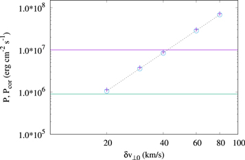
Figure 4. Power per surface unit P transferred to electrons is plotted as a function of δv⊥0 in the case of ΔE∥ with a Gaussian distribution (blue crosses) or with a stretched-exponential distribution (light blue circles). The green and blue horizontal lines correspond to the values of Pcor for quiet-Sun regions and active regions, respectively (Withbroe 1988). The black dashed line represents a function proportional to  .
.
Download figure:
Standard image High-resolution imageAnother relevant feature shown in Figure 4 is that P turns out to be proportional to  . In particular:

where κ ≃ 1.34 × 10⁻¹³ g cm−3. We notice that the scaling law  is remarkably well satisfied by the results, at least for the considered values of the physical parameters (B0, n0, l⊥0, Tp) which characterize the model. Such a scaling law is reminiscent of a property of the mean spectral energy flux
  in a turbulent fluid, which is scale by scale proportional to
 ![${\left[\delta v(l)\right]}^{3}$](https://content.cld.iop.org/journals/0004-637X/871/1/66/revision1/apjaaf168ieqn50.gif) , (Frisch 1995), with δv(l) the velocity fluctuation amplitude at a given scale l. This point will be discussed in more detail in the next section. Finally, from Figure 4 we can observe that, for any given δv⊥0, the same value of P is found using the Gaussian pG or the stretched-exponential pSE distribution for ΔE∥i,m. This indicates that the power transferred to electrons is determined by only the δE∥K value, i.e., the rms of the fluctuating parallel electric field ΔE∥, and not by details of its distributions, a straightforward consequence of the linearity of the acceleration process of the model. In particular, the presence of intermittency does not seem to play any role in determining the power P.
, (Frisch 1995), with δv(l) the velocity fluctuation amplitude at a given scale l. This point will be discussed in more detail in the next section. Finally, from Figure 4 we can observe that, for any given δv⊥0, the same value of P is found using the Gaussian pG or the stretched-exponential pSE distribution for ΔE∥i,m. This indicates that the power transferred to electrons is determined by only the δE∥K value, i.e., the rms of the fluctuating parallel electric field ΔE∥, and not by details of its distributions, a straightforward consequence of the linearity of the acceleration process of the model. In particular, the presence of intermittency does not seem to play any role in determining the power P.
We have also examined how the kinetic energy  is distributed among the population of test electrons. In the upper panel of Figure 5, the kinetic energy distribution
  is plotted at different times, in the case of a Gaussian-distributed ΔE∥ and δv⊥0 = 4 × 106 cm s−1. This panel shows the asymptotic approach of the energy distribution to a power law
  . Therefore, for long times the considered mechanism tends to form a population of accelerated particles at energies much higher than the mean value
  . In the lower panel of Figure 5 the energy distribution
  , calculated at the time
  when the mean energy reaches the value
  , is plotted for different values of δv⊥0. It can be seen that all the distributions corresponding to the same value of
  but different δv⊥0 are essentially superposed. This reveals a self-similarity property of the model: indicating by t* the time when the mean energy
  reaches a given value E'*, and introducing a rescaled time t' = t/t*, then the behavior of the population of test particles depends only on the time t', regardless of the value of δv⊥0. From Figure 5 we can also estimate the value γ ≃ 0.8 of the power-law index associated with
  .
.

Figure 5. The kinetic energy distribution  among the population of electrons is plotted in logarithmic scale. Upper panel:
  is plotted at different times for δv⊥0 = 4 × 106 cm s−1. Lower panel:
  is plotted at the time
  for different values of δv⊥0; the black dashed line corresponds to a function
  . Both panels correspond to the case of a Gaussian-distributed ΔE∥.
Download figure:
Standard image High-resolution image
We have also calculated  in the case of parallel electric field distributed according to the stretched-exponential distribution (16) (not shown). The results are essentially coincident with those of the Gaussian distribution. Therefore, again the presence of intermittency does not seem to influence the overall dynamics of the electron population.
4. Discussion and Conclusions
The properties of KAWs resulting from an MHD turbulent cascade in a typical coronal loop, are suitable to propose the interaction between electrons and KAWs as a possible acceleration mechanism able to heat the solar corona. While the energy flux injected at large scales by photospheric motions is compatible with the power necessary to maintain the coronal plasma at the observed temperature against radiative losses, how such energy is dissipated at small scales is still an open problem. In fact, due to the smallness of collisional dissipative coefficients, the collisional dissipative scale of the turbulence is smaller than typical kinetic scales, such as the proton Larmor radius Rp. As a consequence, it is expected that kinetic effects can play a relevant role in the turbulent energy dissipation and heating. In the present paper we have addressed this point. We have presented a model for stochastic energization of electrons by parallel electric field associated with small-scale fluctuations. In an MHD turbulence there is a tendency to generate small-scale fluctuations with wave vectors nearly perpendicular to the mean magnetic field. This tendency is even better verified in the RMHD approximation, due to the strong background magnetic field and to the prevalence of fluctuations with l⊥ ≫ l∥ already at large scales. RMHD predicts the prevalence of noncompressive fluctuations propagating along B at the Alfvén speed, with Alfvénically correlated velocity and magnetic field fluctuations. On this basis, we expect that in coronal conditions the turbulence at small scales is dominated by KAW-like fluctuations, that can accelerate particles by the associated parallel electric field.
We have modeled the dynamics of single electrons as test particles, which move along a magnetic field in the reference frame locally comoving with the plasma. Each electron is accelerated or decelerated by the parallel electric field associated with fluctuations that propagate along B at the Alfvén speed in both directions. The cumulative effect of a large number of such interactions on a population of electrons is to increase its mean energy in time. In a typical solar coronal loop, this mechanism raises the mean energy of test particles to values of the order of 102 eV, corresponding to typical coronal temperatures, in a time ranging between tens to hundreds of seconds.
A relevant quantity is the power per transverse surface unit P, which particles absorb from fluctuations. The model predicts that P depends on the amplitude δv⊥0 of the velocity fluctuation at large scales. Both observations (Alexander et al. 1998; Brosius et al. 2000; Harra et al. 2001) and models (Nigro et al. 2005; van Ballegooijen et al. 2011) indicate velocity fluctuations in the coronal plasma of the order of a few tens of kilometers per second, which occasionally can rise to ∼102 km s−1 prior to a flare start. For a density n0 = 109 cm−3 and a loop length L = 1010 cm, our model predicts values of P between ∼106 erg cm−2 s−1 and ∼107 erg cm−2 s−1, when δv⊥0 varies in the range 20–40 km s−1. Such values of P favorably compare with those Pcor necessary to keep the coronal plasma at the observed temperature (Withbroe 1988), both for the case of the quiet Sun (Pcor ≃ 8 × 10⁵ erg cm−2 s−1) and for the case of an active region (Pcor ≃ 107 erg cm−2 s−1). Of course, the above values of P depend also on the choice of other parameters of the model, namely, the magnetic field B0, the turbulence injection scale l⊥0 and the proton Larmor radius Rp. A calculation of P as a function of those parameters is left for a future work. However, in the limit of the model's simplifications, our results suggest that the interaction of electrons with KAW-like fluctuations at small scales represents a good candidate to explain particle energization in the coronal turbulence.
From a more general point of view, another interesting feature of the model is the strict proportionality between P and  , which is reminiscent of the dependence of the spectral energy flux on the fluctuation amplitude in a fluid turbulence (Frisch 1995). More specifically, in an incompressible MHD turbulence, under the hypothesis of homogeneity and isotropy, the Politano–Pouquet law holds (Politano & Pouquet 1998):

where  are the Elsässer variables, δf(l) = f(x + l) − f(x) is the running difference of a quantity f over a distance l, angular brackets indicate an average with respect to the position x and the index L indicates the vector component along x. The quantities
  are related to the mean energy flux
  (the power transferred through the spectrum per mass unit) through the relation
  . Performing an order of magnitude estimate, from Equation (19) we derive
 ![$\langle \epsilon \rangle \sim (3/2){\left[\delta v(l)\right]}^{3}/l$](https://content.cld.iop.org/journals/0004-637X/871/1/66/revision1/apjaaf168ieqn72.gif) , where we assumed
, where we assumed  . In our case the turbulent cascade essentially takes place in the perpendicular direction. Therefore, we identify the scale l in the above expressions with l⊥. The corresponding power per transverse surface unit is
  , where L is the longitudinal length of the loop. Evaluating the constant
  at the largest scale l⊥0 we obtain

Equation (20) has the same form as the scaling law (18) for the power absorbed by electrons, and then the two factors κturb and κ can be compared. If κ ≳ κturb, then all the energy carried to small scales by the turbulent cascade is transferred to electrons; on the contrary, if κ < κturb, then electrons absorb only a fraction of the turbulent energy. We estimate κturb by the expression (20), using for n0, l⊥0, and L the same values considered in the model. This gives κturb ≃ 8.3 × 10⁻¹⁴ g cm−3. Comparing with the value κ ≃ 1.34 × 10⁻¹³ g cm−3 found from the model results, we see that κ ≳ κturb. Therefore, we conclude that in the present case most of the turbulent energy is transferred to electrons. In other words, the considered mechanism of electron energization effectively acts as an equivalent kinetic dissipation for turbulence.
In our case the values found for κ and κturb have essentially the same order of magnitude. However, while κturb is determined only by n0 and by the loop aspect ratio L/l⊥0, the coefficient κ in principle could depend also on other parameters characterizing the model, namely, B0 and the proton temperature Tp (or, equivalently, the proton Larmor radius Rp). Hence, there could be other regimes where the present condition κ ≳ κturb is not verified. Exploring the parameter space in a future work could allow us to determine regimes in which the considered mechanism is able to fully dissipate the turbulent energy, and others in which the cascade continues toward smaller scales, where other mechanisms can contribute to remove the turbulent energy.
The model predicts that, with increasing time, the distribution of electron energy  asymptotically tends to a power law. Moreover, the behavior of the energy distribution is independent of the turbulence amplitude (determined by δv⊥0) if time is rescaled to a time t* when the mean energy reaches a given value E'*. It is clear that the form of
  could be different if other effects (like collisions) that tend to thermalize the distribution were included in the model. In such a case it could happen that the distribution is totally thermalized by collisions, or that a tail of nonthermal particles survives at high energies instead. Including the effect of collisions in the model would allow us to discriminate between these two possibilities.
Finally, we remark that in the model the mean energy of the electron population continues to increase in time with no limits. This is due to the lack of any form of energy loss, like radiation. However, since the power absorbed by electrons is compatible with that required to balance radiative losses, we expect that a proper inclusion of energy losses in the model would lead the electron population to a final stationary state where the mean energy corresponds to typical coronal temperatures.
Appendix: Time and Velocity Calculation
In this Appendix, we calculate the expressions of the final velocity u∥1;i,m and time t1;i,m for an electron that interacts with a small-scale fluctuation  . To simplify the notation, in what follows we will drop the subscripts i,m in all the quantities. The fluctuation is characterized by a parallel length l∥K, a propagation velocity σvA (σ = ±1), an electric field amplitude ΔE∥ and a lifetime tL (given by Equation (6)). The electron enters the fluctuation at the initial time t0 with the velocity u0. The electron velocity relative to the fluctuation is indicated by U∥(t) = u∥(t) − σvA, assuming that capital letters indicate the quantities in the reference frame of the fluctuation, while small letters indicate the same quantities in the G' reference frame.
Since ΔE∥ is constant, the parallel motion of the electron in the reference frame of the fluctuation is described by the equations:


where a∥ = −eΔE∥/me is the acceleration, S(t) is the electron position in the reference frame of the fluctuation (defined such as S = 0 at the initial time t = t0), and U∥0 = U∥(t = t0). Note that, if the initial relative velocity U∥0 is positive (negative) then the fluctuation is considered to be located in the interval 0 ≤ S ≤ l∥K (−l∥K ≤ S ≤ 0). If U∥0 and a∥ have opposite signs the electron is decelerated and the relative velocity U∥(t) changes sign at the inversion time tinv = −U∥0/a∥ + t0 (Equation (22)). Correspondingly, in the reference frame of the fluctuation, the electron covers a distance given by (Equation (21):

There can be different possibilities, according to the signs of U∥0 and a∥ and to the value of Linv in comparison with the fluctuation parallel length l∥K. In the following we consider all the possible cases.
(a) U∥0 and a∥ nonvanishing and opposite, and Linv ≤ l∥K.
The first condition indicates that  is a decreasing function of time, and the second condition implies that the motion inversion takes place inside the fluctuation. This case corresponds to a situation when the electron is reflected back by the interaction with the fluctuation. The electron takes time Δta to exit from the fluctuation, given by

with a final relative velocity that is the opposite of the initial one: U∥1 = −U∥0. However, if Δta turns out to be larger than the lifetime tL of the fluctuation, then the time the electron remains inside the fluctuation is tL, and the final velocity is

Summarizing, in the case "a" the final time and velocity are calculated in the following way:
(b) U∥0 and a∥ nonvanishing and opposite, and Linv > l∥K.
In this case the electron is decelerated (as in the case "a"), but there is no motion inversion because the inversion length Linv is larger than the parallel length l∥K of the fluctuation. The final time is calculated by requiring that  , where Δtb is the time the electron takes to go through the whole fluctuation. Using Equation (21), this condition gives:

From Equation (22) we derive the final relative velocity:
Similar to the previous case, if Δtb is larger than the lifetime tL of the fluctuation, then the time when the electron remains inside the fluctuation is tL, and the final velocity is uL (Equation (25)).
Summarizing, in case "b" the final time and velocity are calculated in the following way:
(c) U∥0 and a∥ nonvanishing and with the same sign, or U∥0 = 0 and  .
.
In this case the electron is accelerated, i.e.,  is an increasing function of time. The final time is calculated by requiring that
  , where Δtc is the time the electron takes to go through the whole fluctuation. Using Equation (21), this condition gives:
From Equation (22) we derive the final relative velocity:
If Δtc is larger than the lifetime tL of the fluctuation, then the time the electron remains inside the fluctuation is tL, and the final velocity is uL.
Summarizing, in the case "c" the final time and velocity are calculated in the following way:
(d) a∥ = 0 and  .
.
In this case, the electron crosses the length l∥K with a constant relative velocity U∥0, taking a time given by  . As in the previous cases, we compare Δtd with the lifetime tL. Therefore, the final time and velocity are given by:

(e) a∥ = 0 and U∥0 = 0.
This case is extremely improbable to happen and, whenever verified, it is simply skipped. The numerical procedure generates a new random value for ΔE∥, in order to have  and U∥0 = 0. This new situation corresponds to the case "c."