


Abstract
Current sheets are believed to form in the wakes of erupting flux ropes and to enable the magnetic reconnection responsible for an associated flare. Multiwavelength observations of an eruption on 2017 September 10 show a long, linear feature widely taken as evidence of a current sheet viewed edge-on. The relation between the high-temperature, high-density plasma thus observed and any current sheet is not yet entirely clear. We estimate the magnetic field strength surrounding the sheet and conclude that approximately one-third of all flux in the active region was opened by the eruption. Subsequently decreasing field strength suggests that the open flux closed down over the next several hours through reconnection at a rate  Mx s−1. We find in AIA observations evidence of downward-moving, dark structures analogous to either supra-arcade downflows, more typically observed above flare arcades viewed face-on, or supra-arcade downflowing loops, previously reported in flares viewed in this perspective. These features suggest that the plasma sheet is composed of the magnetic flux retracting after being reconnected high above the arcade. We model flux tube retraction following reconnection to show that this process can generate high densities and temperatures as observed in the plasma sheet. The retracting flux tubes reach their highest temperatures at the end of their retraction, well below the site of reconnection, consistent with previous analysis of AIA and EIS data showing a peak in the plasma temperature near the base of this particular sheet.
Export citation and abstract BibTeX RIS
1. Introduction
Current sheets are an essential element in most solar flare models, including the prevailing CHSKP model of eruptive flares (Carmichael 1964; Sturrock 1968; Hirayama 1974; Kopp & Pneuman 1976), where a current sheet is believed to form in the wake of an erupting flux rope. Most theoretical models require that magnetic reconnection occur at some form of current sheet, where layers of differing magnetic fields are brought into close proximity (Heyn & Semenov 1996; Birn et al. 2001; Biskamp & Schwarz 2001; Vršnak & Skender 2005; Bhattacharjee et al. 2009; Forbes et al. 2013). Under this hypothesis, a current sheet must also be present in compact flares and transient loop brightenings, both believed to be powered by reconnection.
In spite of their central role, only a small number of remote sensing observations have reported current sheets. Most of these have been in the high corona or solar wind (Ciaravella et al. 2002; Ko et al. 2003; Webb et al. 2003; Bemporad et al. 2006; Ciaravella & Raymond 2008; Lin et al. 2015), but a few have been observed above limb flares (Savage et al. 2010; Liu 2013; Seaton et al. 2017). Imaging observations show long, thin linear emission features in white light, EUV, or soft X-ray images, which resemble the expected current sheet viewed from an edge-on perspective. Such features are produced by high-density plasma, rather than by electric current, and are thus more accurately termed plasma sheets. Because of this distinction, observed properties of a plasma sheet, including its apparent thickness, ∼3–30 Mm, cannot be automatically attributed to the current sheet itself.
Assuming a causal connection, the plasma sheet's properties should be somehow related to processes mediated by the current sheet, such as magnetic reconnection. Plasma sheets have temperatures higher than their surroundings, suggesting a heat source within them (Ciaravella et al. 2002; Warren et al. 2018, hereafter W18)—presumably magnetic energy dissipation at the current sheet by laminar shock or turbulent heating (ohmic or viscous). Spectroscopic observations show excess broadening of spectral lines within the plasma sheet, which is attributed to unresolved turbulent flows in and around the current sheet (Ciaravella & Raymond 2008; Li et al. 2018; W18)—turbulence often taken to be driven by magnetic reconnection at the current sheet (Bemporad 2008). Plasma sheets are clearly distinguishable owing to their high emission measure (EM), which reflects a plasma density substantially higher than their surroundings. Few investigations have been able to quantitatively explain or predict this crucial aspect as a direct consequence of magnetic reconnection; doing so is one of the main objectives of the present work.
An eruption and flare on the Sun's west limb on 2017 September 10 exhibited a linear EUV feature of unusual brightness, persistence, and narrowness, suggesting a plasma sheet viewed from a particularly favorable angle. Observed thoroughly by many instruments, this event promises unprecedented insight into the nature of the plasma sheet surrounding a current sheet, and thereby new insights into magnetic reconnection in a solar flare. Consequently, there have already been a number of papers reporting different aspects of the event (Doschek et al. 2018; Gary et al. 2018; Li et al. 2018; Long et al. 2018; Omodei et al. 2018; Seaton & Darnel 2018; W18). Seaton & Darnel (2018) used the SUVI instrument on GOES to track the flux rope and observe the plasma sheet in EUV out to 1.67 R⊙. Gary et al. (2018) used hard X-ray observations from RHESSI (Lin et al. 2002) and microwave observations from the Expanded Owens Valley Solar Array to study the population of nonthermal electrons, primarily in the closed loops below the plasma sheet. W18 used data from Hinode/EIS (Culhane et al. 2007) and SDO/AIA (Lemen et al. 2012) to compute the temperature and turbulent line widths within the plasma sheet itself. Li et al. (2018) use the same data set to map the turbulent velocity through it and measure a thickness of 7–11 Mm.
This diverse set of studies has provided new insight into the structure of a plasma sheet. W18 reported a peak in temperature very close to the sheet's base, which they took as evidence for heating within the sheet. It is tempting to interpret the low peak as the site of the magnetic reconnection. While standard flare models predict a reconnection site near the current sheet's center (Lin & Forbes 2000; Reeves & Forbes 2005), recent theoretical investigations place the null point, and nearby stagnation point, near the lower tip of the current sheet and just above the flare loops (Forbes et al. 2013, 2018), in apparent agreement with the observed temperature peak. W18 also identify and track the top of the plasma sheet, moving upward at ≃288 km s−1, as if it were moving away from the reconnection site. Turbulent line widths appear to increase moving upward (W18) and away from the sheet's center (Li et al. 2018). This has implications for the source of turbulence within the sheet, but they have yet to lead to a definite conclusion. Nor has there been a compelling explanation for the very large density that must exist throughout this long, thin structure in order for it to appear so bright in many EUV bands.
When an eruption is viewed face-on, its trailing plasma sheet appears as a tall, broad, fan-like structure above the post-flare arcade (Švestka et al. 1998), offering complimentary insight. Of particular note are elongated dark structures, called supra-arcade downflows (SADs), observed to move sunward through the plasma sheet (McKenzie & Hudson 1999; Innes et al. 2003; Sheeley et al. 2004; Khan et al. 2007; McKenzie & Savage 2009; Savage & McKenzie 2011; Guo et al. 2013; Reeves et al. 2017). Supra-arcade fans viewed edge-on sometimes exhibit downward-moving loops, called supra-arcade downflowing loops (SADLs) interpreted as SADs viewed from a different perspective (Savage & McKenzie 2011). Both features have been interpreted as magnetic flux tubes retracting sunward following their formation through reconnection at a site higher up (McKenzie & Savage 2009; Savage et al. 2010). An investigation by Savage et al. (2012) suggested that the dark regions forming SADs are actually wakes surrounding the retracting tube. In any case the downflowing features reveal the motion of reconnected flux tubes. Their motion, as well as the motion of the surrounding plasma, has revealed that the sheet is at relatively high plasma β (McKenzie 2013; Scott et al. 2016b) and may be heated by its own compression (Reeves et al. 2017).
In this work we use AIA data and adopt the analysis techniques introduced by W18 to rederive the temperature and density profile of the plasma sheet of the 2017 September 10 eruption. We do this in the next section, where we also produce a version of their time-height stack plot extending higher and lower, and further in time. There we find evidence for sunward-moving dark features, suggestive of SADs or SADLs. We propose that these are, in fact, downflowing loops moving though the plasma sheet. This suggests, however, that reconnection is occurring far higher in the plasma sheet than the observed temperature peak. In the subsequent section, we hypothesize that the retraction of the flux tubes, created by reconnection high above, produces the high density and high temperatures observed in the plasma sheet. In Section 4, we use a thin flux tube (TFT) model of this process to confirm that it is indeed capable of producing sufficiently high densities and temperatures; no other plausible reconnection scenario seems able to do so. We find, moreover, that downward retraction produces higher temperatures lower down, away from the reconnection site, so that the temperature peak is not located at the reconnection site.
2. The Plasma Sheet
The eruptive flare of 2017 September 10 was hosted by AR 12673, when it was about 2◦ over the west limb. In spite of partial occultation, this was an X8.3 flare, peaking at 16:06 (see the bottom panel of Figure 1). It was a long-duration event whose GOES 1–8 Å light curve decayed for over 16 hr before returning to pre-flare levels. The flare was preceded by a coronal mass ejection (CME) whose filament material and flux rope cavity were clearly visible in EUV and are shown in the 15:49 and 15:53 images, respectively, from Figure 1. The eruption created a long, thin, linear feature, which remained visible in EUV for over 4 hr (2 hr are shown in Figure 1). This feature appears to point to the base of the erupting flux rope in exactly the manner predicted by 2D CSHKP models of eruptive flares (Kopp & Pneuman 1976; Lin & Forbes 2000). Matching 2D models so closely would seem to require the viewpoint to be almost precisely parallel to the current sheet. Its properties were measured very carefully by W18 and others (Gary et al. 2018; Li et al. 2018; Seaton & Darnel 2018) and will be the subject of further investigation here.

Figure 1. X8.3 flare on 2017 September 10. At the top are eight images from AIA 193 Å showing stages of the eruption and flaring. Each is plotted on the same logarithmic inverse color scale. Below are plotted the light curves of the total emission from the AR and plasma sheet in 193 Å (black) and GOES 1–8 Å (blue), on linear scales whose axes are on the left and right, respectively. Times of the first seven images are marked by diamonds.
Download figure:
Standard image High-resolution image2.1. Observed Plasma Properties
We obtain characteristics of the plasma sheet following methods similar to those used in W18. Following their methodology, consecutive AIA images made from a long (2 s) exposure and a shorter exposure in the same passband are combined to produce a single image with higher dynamic range and lower noise. The long-exposure images have lower noise but are subject to saturation or even bleeding in some pixels  . We form a single image of a given waveband by combining the x ≥ xco pixels of the long-exposure image with the x < xco pixels of the short-exposure image. An example of such a combined image for the 193 Å bandpass at 16:18 is shown in Figure 2(d). The intensity values of both are normalized to the exposure time (i.e., DN s−1) and match closely where there is no saturation. We have verified that the choice of xco does not affect our results.
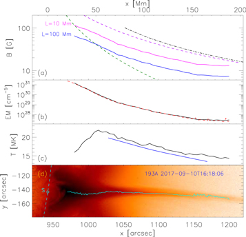
Figure 2. Characteristics of the plasma sheet from 16:18. Panel (d) plots the combined 193 Å image in inverse logarithmic color scale. The cyan curve is the sheet's backbone, from which characteristics were computed. The dashed cyan curve is the limb, and the diamond, labeled S, is the point on the limb directly beneath the plasma sheet. The top axis gives distances in Mm from that point. Panel (c) shows in black Te (in MK) derived in combination with 131 Å images. The temperature derived in W18 using EIS line ratios is shown in blue. Panel (b) shows in black the column EM (in cm−5), derived in combination with 131 Å images. The dashed red curve shows the lower bound on EM from 193 Å alone. Panel (a) shows the magnetic field strength required for confinement, Equation (2), assuming line-of-sight depths of 10 Mm (solid magenta) and 100 Mm (solid blue). Green and violet dashed curves show the field strengths from potential-field and open-field extrapolations, respectively, along a line along the plasma sheet. The black dot-dashed curve above them all is from a simple monopolar field.
Download figure:
Standard image High-resolution imageThe inverse logarithmic color scale of Figure 2(d) shows clearly both the bright arcade (x < 1000'') and the long linear feature extending beyond x = 1200''. This feature is very nearly horizontal, so we make slices through it by extracting vertical columns of pixels. We use the intensity peak to define the backbone of the sheet, shown as a solid cyan curve in Figure 2(d). The intensities of pixels along the backbone, Iλ(x), from bandpasses at 193, 131, and 211 Å, are used to characterize the plasma sheet.
The temperature response, Rλ(Te), for each bandpass is obtained from the SolarSoft tree (Freeland & Handy 1998). We form the column EM curve, Iλ(x)/Rλ(Te), for each bandpass and seek a point of mutual intersection between the three bands. In practice, we identify all intersections between the curves from 193 to 131 Å and use the largest intersection for Te < 40 MK. We then verify that the curve from 211 Å passes near that intersection at points along the entire sheet. In every case it misses the other intersections by a wide margin. The point of intersection is then used as the temperature, Te, and the column EM, at that position and time. The results for 16:18 are shown in Figures 2(b) and (c). Our technique is a crude version of EM-loci method but appears to yield results consistent with those found by W18 using ratios of pure spectral lines observed by EIS and using the complete set of short-wavelength AIA images. That analysis produced a full differential EM, which was found to be narrowly peaked and thus reasonably represented as isothermal. Their values of Te, plotted as a solid blue curve, are systematically ≃1 MK below ours. Among the possible reasons for this are the fact that we did not attempt to remove background intensity because of the effects of the diffraction pattern visible in the image in Figure 2(d). (We consider the results of W18 to be more accurate but have rederived our own version for the detailed model comparisons made below.)
The Te(x) curves from both our analysis and that of W18 have a distinctive peak. At 16:18, shown in Figure 2(c), the temperature peaks, Te,pk = 22 MK, at  . Results from later in the flare (16:41) show a lower peak, Te,pk = 17 MK, at virtually the same height,
  . The EM falls from a very large value EM ∼ 1031 cm−5, with a scale height that appears to increase with altitude. Unlike the temperature, there is very little variation in the EM curve over this first hour of the flare (compare red and blue curves in Figure 3(a)). The EM falls off over scales far shorter than the gravitational scale height, Hp ≃ 1200 Mm for a Te = 20 MK plasma.
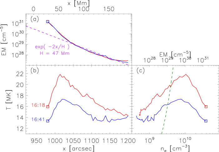
Figure 3. Temperature and EM from 16:18 (red) and 16:41 (blue). The red curves in panels (a) and (b) are the same as shown in Figure 2, while the blue curves are from images 23 minutes later: 16:41. An exponential, with density scale height H = 47 Mm, is plotted against the EM curves for reference. Panel (c) shows Te plotted against density (assuming line-of-sight depth L = 100 Mm). The green dashed line corresponds to an adiabatic line,  , for reference.
Download figure:
Standard image High-resolution imageA vertical slice through the linear feature, plotted in Figure 4(d), gives an indication of the narrowness of the plasma sheet. The intensity peak was used to define the center of the sheet, and the FWHM provides a measure of its thickness. The plot in Figure 4(b) shows that this falls to a level just below Δy ≃ 4 Mm in the vicinity of x ≃ 1100''. The regions above and below may be thicker portions, or may appear wider owing to viewing the sheet from some other angle: the sheet may have a slight twist. At any event the sheet of high-density, high-temperature plasma seems to be no thicker than 4 Mm at its narrowest point.

Figure 4. Width and other characteristics of the plasma sheet from 16:18. Panel (c) shows the 193 Å image as in Figure 2(d). Cyan curves are the points at half maximum, used to define the width. Panel (d), on the right, shows a slice extracted from x = 1070'', shown in panel (c) as a dashed blue line. The FWHM is denoted by a line inside the peak. Panel (b) plots in black the FWHM in arcsec (left) and Mm (right). The widths at a later time are shown in magenta. Panel (a) shows thermal (blue curve) and nonthermal (magenta plus signs) velocities obtained by W18 for the same time.
Download figure:
Standard image High-resolution imageThe width inferred above is far greater than a laminar current sheet broadened by resistivity alone. A Sweet–Parker current sheet of length Δx ≃ 160 Mm and Lunduist number S ∼ 1012, typical of Spitzer resistivity at coronal parameters, would have an aspect ratio of ∼S1/2 ∼ 106 and thus a thickness of less than 1 km. Plasma turbulence can enhance the effective resistivity, leading to a smaller aspect ratio and a thicker sheet. Moreover, W18 report nonthermal line broadening suggesting turbulent velocities exceeding 100 km s−1. Their measurements are plotted as magenta crosses in Figure 4(a). While far greater than a resistive value, the ∼4 Mm thickness we infer is similar to (Savage et al. 2010) or smaller than (Lin et al. 2007; Ciaravella & Raymond 2008; Li et al. 2018) previous observations from this and other events.
2.2. Magnetic Context
Its high density and high temperature mean that the linear feature will have high pressure, which must be confined by the magnetic field around it. The internal plasma pressure can be estimated as
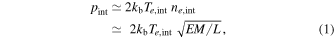
where L is the line-of-sight distance though the sheet—presumably its total width. Confining this entirely through magnetic pressure requires an external field strength no less than

The line-of-sight path, which is not known, enters to a very small power, so two extreme cases, L = 10 Mm and L = 100 Mm, yield a reasonably narrow range of magnetic field strength; these are plotted as solid curves in Figure 2(a).
Computing the actual magnetic field outside the plasma sheet is extremely challenging owing to its location over the limb. To obtain a very rough estimate, we use an SDO/HMI magnetogram (Scherrer et al. 2012) from 4 days before the flare (2017 September 6 11:10) when the host active region was only 36◦ west of central meridian and thus clearly visible. In light of the great uncertainties introduced by this time difference, we opt to use the simplest data: a line-of-sight magnetogram (see Figure 5). The AR is extremely large with roughly balanced fluxes of  Mx in each polarity.

Figure 5. An HMI images from 2017 September 6 used for magnetic context. The line-of-sight field is plotted on a gray scale limited to ±300 G. The yellow curve shows the location of the limb at the time of the flare. Footpoints of a post-flare loop observed on the limb are marked A and B and denoted by cyan crosses. A cyan diamond marks the point directly beneath the plasma slab, labeled S. The red solid curve is the line of sight during the flare. The limb features are moved 30'' to magenta crosses and diamonds, labeled A', B', and S', deemed the likely positions for the footpoints and plasma slab base, respectively.
Download figure:
Standard image High-resolution imageBy the time of the flare, the limb has advanced to lie just east of the AR—the flare was occulted. Footpoints of a single prominent post-flare loop (one of the semi-circular loops visible in the 18:00 panel of Figure 1) are denoted A and B, with cyan crosses. The point on the limb, directly beneath the plasma sheet, is denoted by a cyan diamond labeled S, as shown in Figure 2(d). All three of these points lie on the limb and are therefore outside the AR. Translating all three 22 Mm west from the limb places the footpoints A' and B' squarely within the AR's negative and positive polarities, respectively. We take this to be the likely location of the post-flare footpoints (1 8 behind the limb). We therefore take the point S' to be the photospheric point actually lying directly beneath the plasma sheet.
We perform a potential-field extrapolation from the September 6 magnetogram, shown in Figure 5, and sample it along a vertical line starting at S'. The magnetic field strength along this vertical line, plotted as a green dashed curve in Figure 2(a), falls below the confinement estimate from Equation (2). The curve falls off as a dipole, B ∼ 1/r3, which is evidently faster than confinement requires. The discrepancy is mostly likely due to the neglect, by the potential extrapolation, of the current sheet almost certain to be present in the plasma sheet.
An extreme alternative to potential extrapolation is a completely open field, in which every field line is anchored to the photosphere and extends to infinity (Aly 1992). In a completely open field, regions of inward and outward flux are separated by tangential discontinuities, i.e., current sheets, extending all the way from the photospheric boundary to infinity. The field has no current density except for these. The completely open field is uniquely specified by the radial field at the photospheric surface, Bz(x, y, 0). To compute it, one extrapolates an intermediate field, which is potential and originates in a positive radial boundary given by  . One then arrives at the completely open field by taking this intermediate potential field and reversing the field direction on all field lines actually connected to negative polarity: Bz < 0.
Owing to its current sheets, the field strength of the completely open field, plotted as a violet dashed curve in Figure 2(a), is greater than that of the potential field. Its asymptotic behavior is monopolar,  , as shown by the black dot-dashed curve in the same plot. As the name suggests, the completely open field has open flux,
  Mx. Unlike the potential field, the completely open field has similar form to the minimum confining field (solid curves): it remains above the L = 100 Mm field by roughly a factor of three over most of the run of heights (it exceeds the L = 10 Mm field by a factor of two).
If we posit that the actual field has the minimum strength necessary for confinement, i.e., given by Equation (2), then the completely open field is too strong. This is probably because its current sheets extend all the way from the photospheric surface, in order to keep open the entirety of the AR's flux. A partially open field, in which only one-third of the flux was open, i.e., 7 × 10²¹ Mx of each polarity, would asymptote to a monopolar field strength one-third as large as the completely open asymptote. While we cannot easily compute the partially open field in three dimensions, we believe that it would have roughly one-third the strength of the totally open version, over a range of altitudes. It would therefore better match the minimum confining value over this range. We offer this in support of the hypothesis that the plasma sheet surrounds a current sheet created when the CME opened roughly one-third of the AR's flux. While this is an unusually large fraction (Kazachenko et al. 2017), it is not without precedent (Kazachenko et al. 2012).
By the later time 16:41, shown in Figure 3, the sheet's temperature, and therefore its pressure, had decreased by roughly 22% from its value at 16:18. This would require a confining field smaller by ∼11%, which would, in turn, require a partially open field with 11% less open flux. This suggests that ΔΦ ∼ 8 × 10²⁰ Mx of flux open at 16:18 has been closed down via reconnection at the current sheet during that 23-minute interval. The reconnection would thus be occurring at a mean rate of  . Our indirectly inferred rate compares favorably to values obtained in other flares by observing the motion of flare ribbons (Qiu et al. 2002; Longcope et al. 2010; Tschernitz et al. 2018), particularly during the gradual phase. Reconnection rates have been previously inferred within plasma sheets from the size and frequency of SADs or SADLs (McKenzie & Savage 2009; Savage & McKenzie 2011). The latter measurements have been proposed as lower bounds, since not all retracting flux will produce observable signatures (Savage & McKenzie 2011). Reconnection at the rate we infer would close all open flux,
  , in 4 hr—roughly the life of the plasma sheet. It is presumably this reconnection that sustains the plasma sheet over that long interval. Thus, its observed properties should be consistent with reconnection at
  .
.
2.3. Downflows in the Plasma Sheet
To study the dynamics of the plasma sheet, we construct a stack plot following the method used by W18. In order to follow the sheet to greater heights, we extract pixels from an artificial slit, making a small angle to the pixel directions, as shown in the top panel of Figure 6. A 2-pixel-wide band was extracted using Bresenham's algorithm (Bresenham 1965) to produce the stack plot shown along the bottom panel. The single value in the stack plot is the average of those 2 pixels. To balance the noise level against saturation, we defined a curve in the (t, x) plane below which long-exposure images suffered from saturation. For positions above that we used images with exposure times Δt > 0.15 s. Gaps from the omitted short exposures were filled in using linear extrapolation from earlier and later long-exposure images. Regions below the curve we treated oppositely, using only exposures Δt < 0.15 s and interpolating where reasonable. Short-exposure images were not as plentiful, so the lower section of the stack plot is less smooth in places; this portion was not, however, as important for our study.

Figure 6. Stack plot from the 193 Å sequence. The top panel shows a single image from 16:41, plotted in inverse color, scaled to the 0.2 power to enhance faint features. The cyan line is the line of pixels extracted from each time to produce the stack plot. Magenta triangles mark four locations from which time histories are plotted. The bottom panel shows the entire stack plot using a similar 0.2 power scaling. The blue dashed curve shows the separation between regions constructed with long exposures (above) and short exposures (below). The cyan dashed line, with magenta triangles, is from the time of the top panel. The magenta dashed line, labeled T, is the upward trajectory called out in W18. The green dashed curve, labeled R, is the bottom of the flux rope cavity. The middle panel shows the light curves of the four slit locations indicated by magenta triangles. These are plotted in DN s−1 (left), and a minimum EM is computed assuming Te > 3 MK.
Download figure:
Standard image High-resolution imageOur stack plot is very similar to that of W18 but extends over a wider range of heights and to later times. We overplot, as a magenta dashed line labeled T, the edge they report moving upward at 0 4 s−1. The feature is not as clear in our stack, perhaps owing to our inclined slit.4
The time histories from four horizontal lines, plotted in the middle panel, corroborate our earlier finding that the EM profile remains very steady over times after 16:15.
4 s−1. The feature is not as clear in our stack, perhaps owing to our inclined slit.4
The time histories from four horizontal lines, plotted in the middle panel, corroborate our earlier finding that the EM profile remains very steady over times after 16:15.
Evident in our stack plot, as well as in that of W18, are numerous dark streaks (light in our inverse color table) running down and to the right of line T. These dark, sunward-moving features are reminiscent of the downflows, either SADs or SADLs, mentioned above. SADs have been observed almost exclusively when the arcade, and presumably the plasma sheet, is viewed from a face-on perspective. An edge-on perspective is better for observing the downflowing loops, SADLs, and numerous previous studies have inferred post-reconnection downflows by their presence (Reeves et al. 2008; Savage et al. 2010; Savage & McKenzie 2011). Some previous investigations report aspects of both in particular observations (Liu 2013; Liu et al. 2013; Innes et al. 2014; Seaton et al. 2017). The present observation is similar in many respects to these previous ones.
Extensive studies of both SADs and SADLs have led to the conclusion that these observationally distinct phenomena are manifestations of a single underlying physical process: flux tubes retracting following reconnection higher up. Rather than identify which of the observational phenomena is responsible for the dark streaks we observed, we refer only to downflows or streaks. The key point is that the downflows provide evidence, in this particular plasma sheet, of flux tubes formed by magnetic reconnection occurring higher in the sheet. We aim to use this evidence in explaining the mechanism behind high temperature and high density within the sheet itself.
We perform several processing steps to enhance the dark streaks in the stack plot S(t, x). First, we detrend the array by fitting each time (i.e., column) to a simple exponential

over the range 1020'' < x < 1150''. We then fit the functions a(t) and b(t) to sixth-order polynomials for times after 16:00. We use these fitted functions in the exponential Equation (3), over the full range of times and positions, to produce a smooth trend function, Ssm(t, x). The ratio, H(t, x) = S/Ssm, has values ranging around unity over most of the times and slit positions—it lacks the multiple-order-of-magnitude trend present in S(t, x). Finally, we enhance transient structures by subjecting H(t, x) to unsharp masking. We create a smoothed version by running a Gaussian kernel, with a 90 s width, over each position (i.e., row). We subtract this from the original to produce the detrended, unsharp function ψ(t, x) plotted in Figure 7 using a linear color scale running from blue (negative) to yellow (positive).

Figure 7. Stack plot from the bottom panel of Figure 6 after detrending and unsharp masking. This is plotted in the bottom panel on a linear color scale running from blue to yellow. Some of the dark (i.e., blue) features evident in this processed image are called out, and numbered, in the panel above. A dashed blue line shows the median downward velocity, 330 km s−1, for reference. The dashed magenta curve in both panels separates the long- and short-exposure regions.
Download figure:
Standard image High-resolution imageDownward-moving features are evident as blue streaks in the enhanced stack plot shown in the bottom panel of Figure 7. To call these out, we plot hand-traced curves following the most prominent streaks in the panel above it. It is notable that several streaks cross the exposure boundary (blue dashed curve), although the higher noise level below it makes them harder to track. Of the 35 streaks we traced, 29 were directed downward. Those streaks move downward with a median speed of 330 km s−1 (shown as a dashed blue line in the top panel of Figure 7), and two-thirds below 600 km s−1, comparable to typical speeds observed in SADs (McKenzie & Savage 2009; Savage & McKenzie 2011). There are also a few clear cases of streaks sloping upward, such as no. 23 (immediately above and between the two labeled 22 and 24). While far rarer, there have been observations of upward-moving SADs (Savage et al. 2010)
3. Interpretation of the Observations, and the Challenges Posed
The foregoing observations lead us to a picture summarized in the schematic diagram of Figure 8. The eruption of a flux rope, visible in the 15:53 image of Figure 1, creates a current sheet, depicted as a thick horizontal red line. The current sheet is surrounded by a high-density, high-temperature plasma sheet denoted by a gray box. The stack plot in Figure 6 reveals a gap between the bottom of the flux rope cavity, R, and the top of the plasma sheet, T, suggesting that the plasma sheet surrounds only the lower portion of the current sheet. The cause of the gap must be related to the process responsible for forming the plasma sheet around the current sheet—the focus of this investigation.

Figure 8. Schematic view of the plasma sheet observations. A flux rope erupts to the right, creating an extended current sheet behind it (red thick line). Field lines, shown as blue contours, are anchored to the photosphere, shown as a vertical black line along the left. The plasma sheet is a gray box surrounding the sheet. The scenario is depicted from the edge-on view, as seen in the 2017 September 10 event. Many other observations of SADs have been from the face-on view, indicated by an arrow.
Download figure:
Standard image High-resolution imageThe full extent of the plasma sheet is difficult to know with any certainty. It can be seen extending to the edge of the AIA field of view (x = 1228'') by 16:09. Seaton & Darnel (2018) observed the sheet extending to the edge of SUVI's wider field of view,  , at 16:22. Both are consistent with its top, T, moving at the velocity, v = 04 s−1, measured by W18 (see also the dashed magenta line in Figure 6). If it continued at the same speed, then the plasma sheet would extend from the top of the arcade more than Δxps = 330 Mm by 16:18 and Δxps = 820 Mm by 16:41.
The flux rope itself, by contrast, accelerates through the AIA field of view, leaving at a speed that is difficult to measure. Seaton & Darnel (2018) tracked its center to 1.55 R⊙, at 15:57, in EUV images of SUVI. They find it accelerating throughout, reaching 2000 km s−1 before leaving the field of view. Its bright front is clearly visible in both LASCO coronagraphs, exiting the C2 field (6 R⊙) by 16:24 and the C3 field by 18:54 (30 R⊙). The LASCO CME catalog reports a linear speed of 3.2 Mm s−1 (42 s−1) 10 times greater than the top of the plasma sheet. While this is for the front of the cavity, rather than the bottom point, R, there would appear to be an ever-extending portion of current sheet above the plasma sheet.
Evidence suggests that reconnection occurs at one or more places in the current sheet (magenta crosses in Figure 8), perhaps sporadically. Downflows are created by the field lines retracting downward to the top of the arcade from reconnection points above. The height from which downflow signatures are generally observed to descend, and are observed in our event, requires reconnection relatively high up in the current sheet—at least xrx ≥ 1100'' in our case.
The location of the temperature peak, xpk ≃ 1020'', appears to be well below the reconnection site. Several of the downward-moving streaks move through the x ≃ 1020'' peak completely, most notably nos. 12 and 32. In the event of 2011 October 22, observed from the face-on perspective, Reeves et al. (2017) found temperature peaking in an elongated ridge lying just above the arcade. They observed SADs occurring above it and even passing through it. The temperature does not, therefore, appear to peak at the location of the reconnection.
In most theoretical models, the reconnection site is the X-point at which new magnetic connectivity is forged, but it is not the site of the energy release or the heating. In Sweet–Parker models, heating occurs through ohmic dissipation throughout the entire sheet. In faster Petschek models, heating occurs through shocks that extend a great distance from the X-point. In light of this, it is not entirely surprising that the temperature peak occurs elsewhere. Given that the current sheet may extend well over 1000 Mm upward, even a reconnection site 100 Mm above its base can be considered to be low, and consistent with recent models (Forbes et al. 2018). We are left, in any event, with the open question of why the temperature peak occurs where it does.
The plasma sheet is notable for its high temperature, but is even more remarkable for its high density. Even the most conservative estimate, made assuming a line-of-sight depth of L = 100 Mm, demands electron densities  at z = 50 Mm above the surface. For comparison, an equilibrium 100 Mm coronal loop with
  K at its z = 50 Mm apex would have a density
  there. If we take this to be the ambient density at that height, then creating the sheet would require the surrounding plasma to be compressed by more than an order of magnitude at the same time it is heated. While the presence of high current density can lead naturally to high temperature, it is less clear how it would enhance the plasma density by such a large factor. This poses another challenge for the explanation of the plasma sheet.
3.1. Steady Petschek Reconnection
One possible explanation of the plasma sheet properties worth exploring is that it is the narrow outflow jet from Petscheck reconnection. The slow shocks that bound the outflows in this model both heat and compress it, consistent with the measurement. The increase in its width from Δy ∼ 4 to 12 Mm over Δx ∼ 50 Mm in each direction (see Figure 4) could be explained as the jet's opening angle of

In the standard shock theory, with 1 and 2 denoting pre-shock and post-shock values, respectively, the opening angle is equal to the upstream Alfvén Mach number

where the orientation of the x-axis is along the outflow, as in the observation. This is close to the maximum rate permissible under the Petschek model (Forbes & Priest 1987; Forbes et al. 2013) and is commonly taken to be the prevailing value. Assuming an ambient mass density  and the confining field strength at z = 50 Mm, B = 40 G, gives an inflow speed v1y = 260 km s−1.
The reconnection electric field, Ez = v1yB1x, must be constant along the sheet for the reconnection to be steady. Adopting the values above and integrating the electric field along the assumed width of L = 100 Mm yields a rate of flux transfer

20 time larger than we had inferred. Reconnection at this rate would close all open flux in just 11 minutes, rather than the 4 hr the plasma sheet is observed to persist. It would seem that steady Petschek reconnection is too fast to be consistent with the observations.
It is also the case that the slow magnetosonic shocks in standard models of steady Petschek reconnection produce too much heating and not enough compression to explain the observations. Those models predict an outflow bounded by a limiting slow shock, called a switch-off shock, whose maximum compression ratio is X = 2.5 (see Priest & Forbes 2000). This is smaller than we infer by at least a factor of four. The temperature ratio across the shock is

where  is the plasma β of the upstream plasma. The values quoted above give a post-shock temperature of T2 = 65 T1 = 131 MK, far in excess of what is observed. Moreover, the ratio is proportional to the square of the upstream magnetic field. The downward field strength increase we infer would produce a temperature maximum at the base in agreement with observation. The fourfold increase from x = 150 Mm to x = 50 Mm would, however, produce a 16-fold increase in temperature, while we observe no more than a 30% increase.
While offering a promising explanation of the compression, the heating, and the width of the plasma sheet, it seems that standard quasi-steady Petschek theory fails to quantitatively match the observations. It is notable that the model, which assumes a large-scale, steady electric field, reconnects at a rate 20 times faster than observations warrant. Perhaps if fast, Petschek-like reconnection were active only intermittently, it might better account for what is observed.
3.2. Plasmoid Instability
There has been much recent interest in a class of unsteady reconnection models in which a current sheet is unstable against secondary tearing and devolves into a turbulent layer of magnetic islands called plasmoids (Loureiro et al. 2007; Bhattacharjee et al. 2009; Pucci & Velli 2014; Shibayama et al. 2015; Comisso et al. 2016). The instability and turbulence create an effective diffusivity capable of maintaining the layer at a marginally stable effective Lundquist number, Seff ∼ 104 (Pucci & Velli 2014), for which the current layer will have an aspect ratio  . If this were the case, the 4 Mm wide plasma sheet should extend Δx ∼ 400 Mm, roughly consistent with what we can infer. Moreover, the turbulent velocity would be some fraction of the external Alfvén speed, found above to be vA = 3 Mm s−1. If the turbulent velocity were a few percent of that speed, it would be consistent with the nonthermal velocities measured by W18 (see Figure 4). If this were the case, however, it is puzzling that the turbulent velocity increases with height while the Alfvén speed decreases.
Plasmoids are formed by intermittent reconnection throughout the current sheet. These are advected by the mean reconnection outflow at a fraction of the Alfveń speed. They offer a plausible explanation for SADs and SADLs (Guo et al. 2013), observed to move at 5%–20% of the Alfvén speed. At the end of the turbulent current sheet, the mean outflow will reach a speed nearly matching the external Alfvén speed, vA ∼ 3 Mm s−1. Given the 100:1 aspect ratio of the sheet, the mean inflow will be only 1% of this speed,  . This produces reconnection at a mean rate

far slower than Petschek, and more in line with our observation. If the mean structure of the outflow does resemble the Sweet–Parker model, then its speed will increase steadily as it approaches the base of the current sheet. This is opposite to the general behavior of SADs, which seem to decelerate as they approach the end (Sheeley et al. 2004; Savage et al. 2010; Savage & McKenzie 2011).
The greatest obstacle to further applying the plasmoid models, in their present forms, to our observations is their lack of clear prediction of temperature or density. Many theoretical investigations have used incompressible MHD in order to focus on the mean reconnection rate (Loureiro et al. 2007; Pucci & Velli 2014). While incompressible models do a reasonably good job predicting velocities in slow reconnection, they cannot be used to predict temperature or densities. Shibayama et al. (2015) have used compressible equations and found that the reconnection between neighboring plasmoids resembles the Petschek model, with switch-off shocks extending from each X-point. These would enhance the density by a factor up to the limiting value, X = 2.5, which has been noted above to be too low. Moreover, since they occupy only a small portion of the plasma sheet's volume, the effective density enhancement is likely to be far smaller still.
3.3. Transient, Patchy Reconnection in Three Dimensions
The TFT model of patchy reconnection, originally described by Longcope et al. (2009), offers an approach nicely complementing the models discussed above. It does not describe the reconnection process itself. Instead, it models the dynamical evolution of flux that releases energy once it has been reconnected. Reconnection is assumed to occur very rapidly within a small patch of the existing current sheet. This localized reconnection creates a bent flux tube confined within the otherwise stationary current sheet. The tube retracts under its magnetic tension, sliding between the magnetic layers otherwise separated by the sheet. The magnetic pressure of these layers confines the tube, keeping its internal pressure in balance. Magnetic tension causes the tube to retract at the Alfvén speed and drives flows along its axis at a fraction of that speed. These flows shock, resulting in heated and compressed plasma near the tube's apex.
While they resemble hydrodynamic shocks, rather than switch-off shocks, the resulting evolution has many similarities of Petschek's model under the assumption that reconnecting field lines are skewed rather than being strictly antiparallel (Petschek & Thorne 1967; Soward 1982). If the TFT dynamics are analyzed assuming shock relations, one finds post-shock densities and temperatures in close agreement with the standard Petschek modeling of skewed fields (Longcope et al. 2010). The retracting tube can be considered a single piece of the traditional outflow jet in Petschek's model. In this sense the TFT model can be viewed as a time-dependent, 3D generalization of Petschek reconnection. Since the plasma is confined to the axis of the flux tube, albeit an evolving axis, its dynamics can be modeled with the same resolution and fidelity as in standard 1D flare models (Bradshaw & Mason 2003; Allred et al. 2005). Thermal conduction occurs strictly along the field line and drives evaporation from a chromosphere orders of magnitude denser and cooler than the corona. These aspects of the post-reconnection dynamics are essential in making comparisons to flare observations, which are often dominated by evaporated plasma (Longcope et al. 2016). Most significantly, under the TFT model, the flaring loop is energized by the magnetic energy released by retraction of the post-reconnection flux tube.
Retracting flux tubes are a common interpretation of SADs and SADLs (McKenzie & Savage 2009; Savage & McKenzie 2011), so the TFT is a natural model when they are present. The cross section of a flux tube at its apex resembles a plasmoid, so the TFT might also be considered a 3D generalization of that class of models. One key distinction is that the legs of the TFT provide the magnetic tension driving its retraction, while the magnetic island is moved passively by the outflows from neighboring X-points (Shibayama et al. 2015). Its reduction in length is the source of a tube's magnetic energy and a source of plasma compression. These aspects are entirely absent from traditional 2D plasmoid models, where energy and compression arise mainly from the circularization of magnetic islands.
Numerical solutions of the TFT model, most recently done using the PREFT code (Longcope & Klimchuk 2015), have revealed several aspects that promise to explain the plasma sheet described above. Field-aligned thermal conduction moves heat away from the gasdynamic shocks and down the legs of the tube. This results in a central region of lower temperature and higher density than steady shock models predict (Longcope & Guidoni 2011). Compression ratios often exceed a factor of 10, while steady models predict a limit of four. The compressed region is confined to a tube lying within the current sheet, confined by the external layers of flux. The temperature evolves during the retraction and can increase as the tube moves downward from the point of reconnection. This could explain the peak in temperature near the base of the plasma sheet. We perform a TFT simulation in order to explore this promising avenue.
4. Modeling the Plasma Sheet Using Retracting Flux Tubes
4.1. A TFT Simulation
The TFT model tracks the axis of the reconnected flux tube,  , where ℓ is the arc length coordinate. A fluid element in the tube accelerates under the influences of the Lorentz force, pressure p, gravity
  , and viscosity μ, according to (Longcope & Klimchuk 2015)
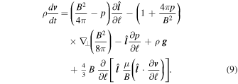
Pressure provides the primary force directed along the tube's tangent vector  = ∂
= ∂ /∂ℓ, while the magnetic tension is proportional to the curvature vector ∂
 /∂ℓ perpendicular to it. The gradient in magnetic pressure also acts perpendicular to the axis, via the perpendicular gradient operator ∇⊥.
The magnetic field strength inside the tube is determined by the layers of flux surrounding the current sheet. We take this to approximately match the values inferred from the AIA data, assuming a line-of-sight depth of L = 100 Mm, shown in blue in Figure 2(a). For expediency we use an exponential fit

where B0 = 50 G and h = 54 Mm. The upward coordinate here is x, as in the observations, but x = 0 Mm, in the simulation, represents the chromosphere, and x = 40 Mm is the base of the current sheet. We assume β ≪ 1 in order to take the tube's internal field strength to match the external field strength B( ) from Equation (10). We will see below that β inside the tube does become large, even exceeding unity, thus violating our assumption. Nevertheless, the underlying forces at work in Equation (9) are still captured by this version of the TFT, provided that β < 2, so that the tension force remains tensile.
The flux tube is broken into elements with fixed mass per magnetic flux, δm, which are followed dynamically. The mass density in an element with length δℓ is found at each time as

The plasma pressure is  , assuming fully ionized plasma with mean particle mass
  (where mp is the proton mass).
The temperature of a fluid element evolves according to the energy equation
including, reading from the equals sign, adiabatic compression, thermal conduction, optically thin radiative losses, and viscous dissipation. We take the radiative loss function, Λ(T), from the output of Chianti 7.1 with coronal abundances and default ionization equilibria (Dere et al. 1997; Landi et al. 2013). Assuming full ionization yields an electron density ne = 0.874(ρ/mp) and specific heat  . Thermal conduction is taken to be classical with a flux limiter at high gradients (Longcope & Klimchuk 2015).
The model is initiated with a flux tube bent at its apex as would be created by reconnection at a point xrx = 120 Mm above the chromosphere. We assume that the flux layers have some field component, Bz(x), parallel to the line of sight (sometimes called a "guide field"). We choose its value to make the angle between flux layers  at the reconnection site, as shown in Figure 9(d). For simplicity, we take the tube to be in mechanical and thermal equilibrium away from the bend. This requirement dictates both magnetic field components, subject to the requirement that
  , given by Equation (10). It also fixes the temperature and density profiles, once one has been prescribed at the apex. We choose an equilibrium with electron density
  , at the apex so that T = 3.7 MK there.
Figure 9. View of the flux tube retracting under TFT dynamics. Panel (d) shows a face-on view of the flux tube axis, as solid curves at times spaced by 9.0 s. Symbols show the apex where the density is maximum, and the section with density above half of the maximum is shaded red. Panel (c) shows the apex density, ne, in red, with symbols at the 9.0 s samples. Blue and green curves show the values along the entire axis at time t = 0 (blue) and t = 36.0 s. (green). The magenta curve shows the initial apex density enhanced in proportion to B; the value of B at the apex can thus be read off the right axis. Panel (b) shows T at the apex (red), along the axis at t = 0 (blue), and at t = 36 s (green). The magenta curve shows the shock-enhanced value given by Equation (7). Panel (a) shows the apex velocity vap (red) and the x component of the Alfvén speed (violet).
Download figure:
Standard image High-resolution imageThis initial tube evolves under the TFT equations described above. Figure 9(d) shows the evolution of the axis, from a face-on perspective, as it retracts leftward—toward the Sun. As it retracts, density is enhanced in a region around the apex, as shown by the red sections of the axis curves in Figure 9(d) and the green curve in Figure 9(c). This compression heats the plasma, and conduction carries the heat downward as evident in Figure 9(b).
A novel feature of our solution is the magnetic field strength increasing downward, as inferred from Figure 2 and captured in Equation (10). This has a number of significant effects on the dynamics, not present in previous studies. Figure 9(a) shows the Alfvén speed (violet) increasing and with it the speed of the tube apex, vap (red). The increasing retraction speed leads to stronger shocks and thus apex temperatures increasing downward, as evident in the red curve of Figure 9(b). Due to the increasingly effective thermal conduction, the rate of increase is far lower than predicted by standard shock relations, reflected in Equation (7) and plotted in magenta. Nevertheless, the temperature rises by roughly a factor of three, which is far more than observed.
Being dragged into regions of increasing B will increase the tube's apex density. In a perfectly horizontal tube ne ∝ B, as indicated by the magenta curve in Figure 9(c). The actual apex density (red) follows this trend, but higher by roughly a factor of 4–6 owing to the shock. The combination of these effects leads to a 20-fold density enhancement, which is large enough to approach the observations.
The field strength rises from B = 11 G, at the initial apex (x = xrx = 120 Mm), to B = 50 G at x = 40 Mm, according to Equation (10). As a consequence, the plasma β of the initial tube drops from β = 0.1 to 0.01. The heating and compression drive β at the tube apex to very large values. It reaches β = 1.56 by t = 11.4 s and thereafter falls gradually to just below unity. These large values do violate the assumption made when fixing the interior tube strength. The plasma β does, however, remain below 2, so the tension force is still able to produce retraction. While challenging the low-β assumption, these marginal values do conform to our assumption of confinement by the surrounding magnetic field.
By t ≃ 72 s the tube has retracted to the point where its apex is at x = 40 Mm, as shown in Figure 9(d). Its axis length has been reduced by Δℓ = 140 Mm, and its magnetic energy,

has dropped by  erg Mx−1. This is the energy source driving the heating and compression in the present TFT model.
Heat generated by shocks at the apex is conducted downward. The conductivity takes the classical Spitzer form  , except where large temperature gradients demand a flux limiter (Longcope & Klimchuk 2015). The conduction front has reached x ≃ 40 Mm by t = 36 s (green curve in Figure 9(c)). By t ≃ 50 s it reaches the chromosphere (not shown) and begins to drive evaporation. The upflow speed is less than 1000 km s−1 and thus requires more than an additional 40 s to reach our x ≃ 40 Mm. We thus see no effect from evaporation in Figure 9. This kind of delay makes evaporation a problematic mechanism for explaining the high density of a plasma sheet.5
4.2. Synthesizing a Plasma Sheet
The simulation above shows how a single flux tube will develop high density and high temperature as it retracts following its creation by reconnection. We propose that the high-density, high-temperature plasma sheet we observe is composed of many such tubes in various stages of retraction. In order to apply this hypothesis, we assign to each tube a fixed flux  Mx, roughly consistent with the Δy = 4 Mm diameter of the sheet. Such tubes must be produced at the rate needed to achieve the mean flux transfer rate
  Mx s−1, inferred from observations. Tubes are thus forged by reconnection with a mean interval
  . The local Petschek reconnection electric field we inferred in Section 3.1,
  Mx s−1, would create a single flux tube in 0.1 s. This very fast reconnection process appears to be inactive 95% of the time, leading to a mean rate 20 times smaller. We have no a priori model for this factor, but adopt the value provided by observation. (This reminds us that in our nonsteady model, the global, observed flux transfer rate
  is fundamentally different from the local reconnection electric field.)
The observed plasma sheet is thus composed of about 40 flux tubes in different stages of retraction following their births at different times. The vast majority of these tubes are not evident as distinct dark streaks in Figure 7, but their aggregated hot dense material forms the plasma sheet. Each tube evolves independently in a similar fashion, like the one simulated above. We thus synthesize the plasma sheet by superposing clones of that single simulated tube at different evolutionary times.
The configuration of the simulated tube at time tj represents the configuration, at time  , of a particular tube j, if it had reconnected at t = −tj. Figure 10(d) shows the tube at tj = 36.0 s viewed in face-on perspective, with a slightly compressed z coordinate. The tube's axis is given by the curve
  (ℓ, tj), and its radius at arc length coordinate ℓ is

where B( ) is from Equation (10). It is evident from Figure 10(d) that the tube's radius increases as the field strength decreases with height. The value of electron density within the tube is taken from its value at the axis position in the simulation, ne(ℓ, tj), shown in the green curve in Figure 10(b). The volume-filling density is shown in Figure 10(d) using an inverse logarithmic color scale. The shocks produce a sixfold density enhancement near the apex, which is evident in both plots.

Figure 10. Single flux tube at tj = 36.0 s. Panel (d) shows the tube viewed from the face-on perspective with compressed z-axis. The local density is indicated in inverse logarithmic color scale: dark is high density. Blue vertical lines show two lines of sight in the edge-on perspective. Panel (c) plots, as a black curve, the total sight line at any point. Two blue plus signs show the values for the lines of sight called out in panel (d). The violet curve is four times the local radius (4a), which is an estimate of the sight line through two legs of the loop. Panel (b) shows the electron density, ne(x), which reproduces the value plotted in color in panel (d). Panel (a) shows the column EM for each sight line.
Download figure:
Standard image High-resolution imageWhen tube j is viewed edge-on, the column EM it contributes to the sight line (x, y) is

and is plotted in Figure 10(a) for the sheet's midplane, y = 0. Two particular sight lines are indicated by vertical blue lines in Figure 10(d). The right one (x = 88 Mm) passes through an Lj = 10 Mm segment near the apex. The left sight line (x = 70 Mm) passes through both legs for a total path of Lj = 5 Mm. These values are plotted as blue plus signs in Figure 10(c), along with the path lengths Lj(x) for the entire tube (black curve). Most sight lines pass only through the legs, giving them a path ≃4a, plotted as a violet line. In the vicinity of the apex, however, the path is longer, giving Lj(x) a bump there. The combination of this longer path and higher density produces an enhancement in EMj(x, 0) of more than 100, as seen in Figure 10(a).
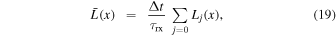
EM contributions, EMj(x, y), from different tubes j = 0, 1, ... are combined into a composite plasma sheet. The sheet at a given time, say, t = 0, will consist of tubes that had reconnected at times −tj ≤ 0. The birth times of successive tubes are separated by tj−tj−1 = Δt = τrx. We produce a smoother composite function by taking a smaller spacing Δt and weighting the contributions accordingly,
The final version of the expression shows how the limit Δt → 0 would result in an integral giving a convolution of the EM per flux with the reconnection rate  (Longcope et al. 2016). The result for the midplane, EM(x, 0), is plotted in red in the bottom panel of Figure 11, for Δt = 0.5 s. Curves, EMj(x, 0), from select times, tj, are plotted in blue.

Figure 11. Synthesis of a plasma sheet from a single flux tube simulation. Images from the top are edge-on views of the tube at five different times, tj, labeled on their right. The column emission measure, EMj(x, y), from Equation (15) is depicted in inverse logarithmic color scale, darker being higher EM. The image below these snapshots shows the composite, EM(x, y), from Equation (16), similarly plotted. In the bottom panel is plotted the individual EMj(x, 0), in blue, and the composite EM(x, 0), in red, both evaluated along the midplane.
Download figure:
Standard image High-resolution imageOther properties of the plasma sheet can be computed using a similar strategy. The EM-weighted temperature of the sheet,
is plotted in black in Figure 12(b). This remains close to, but slightly below, the apex temperature of the tube plotted in red, reproduced from Figure 9(b). The EM-weighted version includes contributions from the legs and regions away from the apex. Evidently, the higher density of the apex makes the temperature there the dominant contribution.
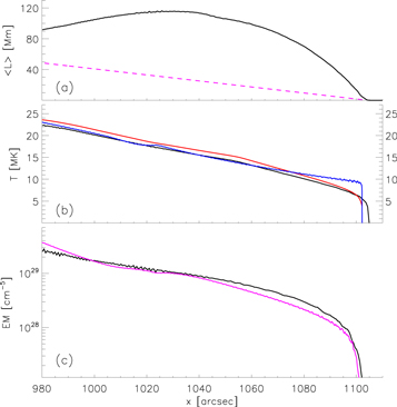
Figure 12. Properties of the synthesized plasma sheet. Panel (c) plots in black the column EM in the midplane. Magenta shows the estimate EM(est), from Equation (20). Panel (b) plots in black the EM-weighted temperature, defined in Equation (17). The red curve shows the apex temperature of the retracted tube, the same curve potted in red in Figure 9(b). The blue curve shows the estimate from Equation (22). Panel (a) shows the mean sight line,  , from Equation (19), plotted in black, and the inter-leg separation, Δz(x), from Equation (18), as a dashed magenta line.
Download figure:
Standard image High-resolution imageThe sight line at point x passes through a path length Lj(x) of tube j, as illustrated in Figure 10(c). When passing though the legs, this is roughly four times the tube radius, shown by the violet line there. The path through the apex cannot exceed the distance between the legs,

The mean path through all of the tubes
plotted in black in Figure 10(a), is considerably larger than Δz(x), plotted as a dashed magenta line. Since  remains below 120 Mm, the collection of all 40 flux tubes could lie side by side in a current sheet of that width. This is not far off the value L = 100 Mm used in foregoing sections.
4.3. Reconciling Discrepancies with Observations
The peak density, at the tube apex, ne,ap(x), is seen in Figure 9(c) to rise by about a factor of four owing to the increase in magnetic field strength B. The apex sight length rises by at least a factor of two from xrx to the end of retraction. We might therefore expect the composite column EM to increase by a factor of 30. Instead, the black curve in Figure 12(c) shows it to rise by only a factor of 10. The discrepancy comes from the fact that the tube is moving faster at the bottom and therefore contributes less to the EM there. A simple estimate that accounts for this factor,

plotted in magenta in Figure 12(c), agrees remarkably well with the composite EM. This expression shows the observed EM to be proportional to the global reconnection rate,  , through τrx, and inversely proportional to the retraction speed of a typical tube. The retraction speed, shown in Figure 9(a), increases by a factor of two to vap ≃ 2000 km s−1 at the base, reducing the EM there by a factor of two.
The retraction velocity in our model differs notably from the downflow streaks, which led us to the reconnection model in the first place. While the model retraction speed increases to vap = 2000 km s−1 at the plasma sheet base, the streaks in Figure 7 have a median speed of 330 km s−1 and appear to slow toward the base: compare the magenta and the blue curves in Figure 13(a). The peak retraction speed is a significant fraction of the Alfvén speed in our model, as well as in most models of magnetic reconnection (compare red and violet curves in Figure 9(a)). Virtually all observed signatures of reconnection outflow, including SADs and SADLs, have velocities far lower than the local Alfvén speed (Savage & McKenzie 2011). The current observations are just the latest in this persistent discrepancy, still lacking an accepted explanation. We return in the Discussion section below to consider several possibilities, but for the moment we accept the fact that vap is overestimated in our model.
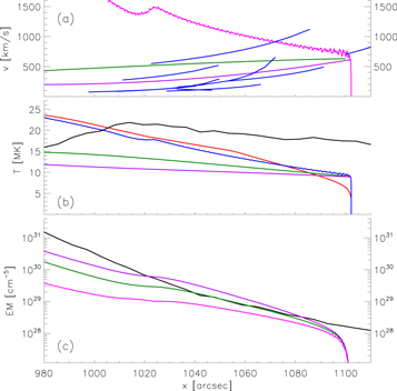
Figure 13. Effects of decreased retraction velocity. Panel (a) shows the retraction velocity, in magenta, and the velocity tracks of several stack plot streaks from Figure 7, in blue. Two alternative velocity tracks are shown in green and violet. Panel (b) shows the temperature profiles from Figure 12(b) in red and blue. The version derived from AIA 193 and 131 Å images, shown in Figure 2(c), is plotted in black. The versions from the modified velocity tracks are plotted in green and violet. Panel (c) plots in magenta the estimated EM from Equation (20) and in black the observed value from Figure 2(c). The versions from the modified velocity tracks are plotted in green and violet.
Download figure:
Standard image High-resolution image
The dependence of EM on retraction velocity offers the possibility of explaining various discrepancies between the model and the observation. The composite EM plotted in Figure 12(c) rises to ≃3 × 1029 at x = 980'', while the observed value, the black curve in Figure 13(c), is more than an order of magnitude greater there. If the retraction velocity were somehow reduced by an order of magnitude in Equation (20), the EM would be increased to a value agreeing with observations. The green and violet curves in Figure 13(c) show this effect.
The EM-weighted temperature rises to just over 22 MK moving away from the reconnection site (xrx = 1100''), in conformance with observations. The model value rises by a factor of three from top to bottom, far more than observed (compare black and red curves in Figure 13(b)). This factor of three rise is, however, far lower than the standard shock model predicts (magenta line in Figure 9(b)), in spite of the fact that our model is heated by shocks. This is due to thermal conduction, ignored in shock relations, which transports heat away from the shocks to the loop's footpoints. The retraction at velocity vap releases magnetic energy to produce the energy flux

heating the plasma sheet. Conduction, with conductivity  , will move the energy a distance ℓap to the footpoints, demanding an apex temperature

where CF is of order unity. This estimate, plotted in blue in Figures 12(b) and 13(b), agrees very well with the simulation, especially in regions away from the reconnection site, where quasi-steady energy balance obtains.
Thermal conduction reduces the temperature variation to levels below that predicted by shock relations, but not to the level comparable to those observed. In the model, where vap ∼ vA ∼ B, the apex temperature will vary as  . This dependence is weaker than the
  dependence from shock relations, Equation (7), and is actually weaker still since ℓap scales inversely with B. It is evident by comparing the black and blue curves in Figure 13(b) that even this weaker dependence on B produces more variation than observed. If, however, the retraction speed vap is taken to increase with height, as do SADs and SADLs, then the apex temperature (green and violet curves in Figure 13(b)) varies far less, in agreement with observations. For the simulation at hand, the level is then lower than observed, but serves to show how the trend is consistent provided that flux retracts at observed sub-Alfvénic speeds.
5. Discussion
We have followed the methodology of W18 to obtain from SDO/AIA data the plasma properties in the plasma sheet of 2017 September 10. We used these, along with an assumption of marginal magnetic confinement, to estimate the magnetic field strength outside the sheet. Our estimate is consistent with a partially open magnetic field, provided that the eruption had opened about one-third of the flux in the AR (i.e.,  Mx). If the observed decrease in the sheet's internal pressure were matched by a decrease in external field strength, then the open field would be decreasing at a rate
  Mx s−1. This rate is consistent with complete closure over 4 hr, the observed life of the plasma sheet. We therefore propose that the plasma sheet results from reconnection occurring at a current sheet created in the wake of the eruption.
A height–time stack plot along a strip of AIA pixels inclined to follow the plasma sheet showed sunward-moving dark features. We propose that these are an edge-on view of downflows (SADs or SADLs) commonly attributed to flux tube retraction following reconnection. Under this interpretation, the site of magnetic reconnection must be higher in the plasma sheet than the point near the base where the temperature peaks. Nevertheless, this higher site (say, 50 Mm above the arcade) can still be considered to be near the base of the current sheet, which we estimate to be over 1000 Mm long by the end of our stack plot. The plasma sheet itself is composed of numerous flux tubes in various stages of retracting throughout the current sheet.
To support our hypothesis, we performed a TFT simulation of a reconnected flux tube retracting through the current sheet. A plasma sheet synthesized from this simulation had high EM and high temperature that increased downward, in qualitative agreement with observations. The synthesized sheet had EM lower than observed and a temperature increase greater than observed. We suggest that the source of both discrepancies is that the model retraction speeds are far higher than SADs or SADLs are found to descend. Similar discrepancies are common to most models of magnetic reconnection: outflows are predicted to be at or near the local Alfvén speed, while outflow signatures, including SADs and SADLs, move far more slowly.
There are several plausible explanations for the very sub-Alfvénic outflows from flare reconnection.6 One issue with the TFT is our use of magnetic pressure balance (i.e., equating internal and external magnetic pressure) in place of total pressure balance. This is done to make the model simpler, and computationally faster, but it leads to internal field strengths larger than would occur in reality. Lower field strength inside a retracting tube would yield a lower Alfvén speed, and possibly a slower retraction. In an extreme case the internal field strength would become so low that the tube itself would lose cohesion and become part of a tangled, high-β slab through which other tubes must retract. This picture seems consistent with the measurements of high β made by McKenzie (2013) and Scott et al. (2016a). In order to confirm this suggestion, the TFT equations would need to be reworked to use total pressure balance in place of magnetic pressure balance.
A second, but related, matter concerns the assumption made in the TFT that a flux tube moves through an ideal current sheet, unimpeded by its surroundings. Notably absent from the momentum Equation (9) is any form of aerodynamic drag. This would be justified if the tube were sliding between two flux layers with nothing else between them. It would not apply, however, if the external layers were separated by an interstitial layer of high-β plasma, or filled with other retracting tubes. In that case, the retracting tube would experience a drag force as it did work moving the material through which it passed. A drag force of this kind, modeled on aerodynamics, has been used in TFT models of flux tubes in the high-β convection zone (Choudhuri & Gilman 1987; Fan et al. 1993). Drag has been previously invoked to explain the sub-Alfvénic speed and deceleration of SADs and SADLs (Savage et al. 2010; Savage & McKenzie 2011). Extending the aerodynamic analogy, we would expect the work done on the surroundings to generate turbulence there. The turbulent velocity would be some fraction of the tube's own velocity and would thus decrease as the tube itself was slowed by the drag. Both expectations agree roughly with the observed turbulent velocity shown in Figure 4(a). Finally, an interstitial layer filled with magnetic turbulence could produce nonthermal electrons via stochastic acceleration (Petrosian 2012), thereby explaining one more of the observations (Gary et al. 2018).
The aforementioned effects leading to sub-Afvénic reconnection outflows lie outside our present TFT model and cannot yet be explored in detail. They are basically modifications of the present TFT model, so we believe that the simulations presented here offer a reasonable starting point for predicting the plasma sheet properties. The sheet would still consist of flux tubes that had been energized and compressed by the process of post-reconnection retraction. The simulation and synthesis we present here confirm that post-reconnection retraction is capable of producing high densities and temperatures. We therefore offer this scenario as a possible explanation of the plasma sheet.
The retracting flux tube hypothesis also predicts total energy release in rough agreement with observations, where competing models do not provide predictions so readily. The simulated flux tube described in Section 4.1 deceases its axis length by Δℓ = 140 Mm, thereby reducing its magnetic energy by ΔWM = 1.9 × 10¹⁰ erg Mx−1. If all the open flux,  Mx, retracted similarly following its closure by reconnection, it would release a total magnetic energy
  erg. Our open flux estimate was made just after the flare's impulsive phase (16:18), so the flux initially opened may be somewhat larger, leading to a slightly larger magnetic energy. Light curves from GOES can be used to compute the temperature and EM of the entire flare plasma, under an isothermal assumption (see W18). From this we compute the total power radiated by the X-ray plasma to be
  erg. The energy conducted to the chromosphere and radiated from there will be at least this large (Kazachenko et al. 2012). The total is therefore approximately explained by the release of magnetic energy via flux tube retraction. Had reconnection occurred lower down, however, the tubes would retract less and release less magnetic energy. Such a lower reconnection site would therefore be hard to reconcile with the flare's observed energy.
This work was supported partly by a grant from NASA's Heliophysics Supporting Research (HSR) program and partly by a grant from NSF/AGS's Research Experiences for Undergraduates (REU) program. We thank Dr. Anna Malanushenko for help with the Bresenham algorithm. We also thank the referee for suggestions that improved the manuscript.
Footnotes
- 4
Placing our line in precisely the same position proved difficult owing to both the different slit configurations and a discrepancy in the ordinates of our graphs.
- 5
W18 use abundance measurements to conclude that the 2017 September 10 plasma sheet contains no evaporated material.
- 6
Priest (2014) offers still another possible explanation invoking a pressure difference through the current sheet. It is not, however, easily applied to the TFT model.