


Abstract
To test a technique to be used on the white-light imager onboard the recently launched Parker Solar Probe mission, we performed a numerical differentiation of the brightness profiles along the photometric axis of the F-corona models that are derived from STEREO Ahead Sun Earth Connection Heliospheric Investigation observations recorded with the HI-1 instrument between 2007 December and 2014 March. We found a consistent pattern in the derivatives that can be observed from any S/C longitude between about 18° and 23° elongation with a maximum at about 21°. These findings indicate the presence of a circumsolar dust density enhancement that peaks at about 23° elongation. A straightforward integration of the excess signal in the derivative space indicates that the brightness increase over the background F-corona is on the order of 1.5%–2.5%, which implies an excess dust density of about 3%–5% at the center of the ring. This study has also revealed (1) a large-scale azimuthal modulation of the inner boundary of the pattern, which is in clear association with Mercury's orbit; and (2) a localized modulation of the inner boundary that is attributable to the dust trail of Comet 2P/Encke, which occurs near ecliptic longitudes corresponding to the crossing of Encke's and Mercury's orbital paths. Moreover, evidence of dust near the S/C in two restricted ranges of ecliptic longitudes has also been revealed by this technique, which is attributable to the dust trails of (1) comet 73P/Schwassmann–Wachmann 3, and (2) 169P/NEAT.
Export citation and abstract BibTeX RIS
1. Introduction
White-light observations of the interplanetary medium between 4° and 88 7 elongation have routinely been carried out from near 1 au since the beginning of 2007 by the combined imaging capabilities of the heliospheric imagers (HI-1 and HI-2, Eyles et al. 2009) of the Sun Earth Connection Heliospheric Investigation (SECCHI; Howard et al. 2008) on the STEREO mission (Kaiser et al. 2008). These instruments record the photospheric light scattered by electrons (the K-corona, e.g., Billings 1966) and by dust particles (the F-corona, Grotrian 1934) in spectral bandpasses of 630–730 nm (HI-1) and 400–1000 nm (HI-2).
Due to the nature of the F-coronal brightness, which results from the interdependence between the density and the scattering properties of the dust grains along the line of sight (see., e.g., Lamy & Perrin 1986), white-light observations (total brightness) do not shed much information on the properties of the dust grains. However, they can reveal the presence of dust density inhomogeneities. For instance, from a re-analysis of data from the Zodiacal Light Photometers experiment (ZLP, Leinert et al. 1975) onboard the Helios mission (Porsche 1981), Leinert & Moster (2007) reported observational evidence of an enhancement in the density of the interplanetary dust cloud near the orbit of Venus. This observational finding was later confirmed by Jones et al. (2013) using two years of data from the HI-2 heliospheric imager onboard the STEREO Ahead spacecraft (hereafter ST-A). More recently, Jones et al. (2017) performed a very extensive mapping of the circumsolar dust ring near the orbit of Venus using 8 years worth of data from the two heliospheric imagers on the twin STEREO S/C. From their analysis of the white-light observations, they found that the inclination of the ring was 21 and the longitude of its orbital ascending node was 685. They noted that: (1) the derived orbital parameters of the dust ring differed from those of Venus (34 and 767, respectively), and (2) the location of the maxima of dust densities differed from the expectations of the theoretical models.
The trapping of particles due to planetary gravitation was first suggested in Gold's (1975) prescient article. Gravitational perturbations near a planet can trap the dust particles in the Zodiacal dust cloud into exterior mean-motion resonances (see, e.g., Weidenschilling & Jackson 1993); thereby, stabilizing their orbital decay due to drag forces, such as solar wind drag (Minato et al. 2004, 2006) and Poynting–Robertson (Poynting 1903; Robertson 1937). Based on numerical simulations of these physical processes, Jackson & Zook (1989) first predicted the existence of a circumsolar dust ring with the Earth as its shepherd. Later on, numerical modeling of Infrared Astronomical Satellite (IRAS) data (Neugebauer et al. 1984) indicated that the Earth ring would exhibit a signature of enhanced density in the direction opposite to the Earth motion (Dermott et al. 1994). The existence of the dust ring just outside the orbit of Earth was finally confirmed by Reach et al. (1995) with data from the Diffuse Infrared Background Experiment (DIRBE, Silverberg et al. 1993; Hauser et al. 1998) on the Cosmic Background Explorer mission (COBE; Boggess et al. 1992). More recently, Reach (2010) measured the azimuthal structure of the resonant dust ring using infrared data from the Spitzer telescope (Werner et al. 2004). He found it to be asymmetric, which is in agreement with dust spiraling inward under the influence of Poynting–Robertson like drag forces.
The upcoming white-light data from the WISPR instrument (Wide-Field Imager for Solar Probe; Vourlidas et al. 2016) onboard the recently launched (2018 August 12) Parker Solar Probe mission (formerly Solar Probe Plus; Fox et al. 2016) has brought to attention the complex issue of the separation of the F- and K-coronal components (see, e.g., Stenborg & Howard 2017a), and the consequent analysis of the geometrical (Stenborg & Howard 2017b; Stauffer et al. 2018) and brightness (Stenborg et al. 2018) properties of the F-corona component. In particular, in Stenborg et al. (2018), we analyzed and characterized the helioecliptic longitude dependence of the brightness profile of the photometric axis of the white-light F-corona between 5° and 24° elongation during the time period between 2007 December through 2014 March. In that work, we modeled the F-corona brightness following a strategy devised and implemented in Stenborg & Howard (2017a, 2017b) from images recorded by the ST-A/HI-1 instrument. On that occasion, we did not look specifically for signatures of dust density inhomogeneities in the brightness profiles. In this paper, motivated by the observational evidence in white-light imaging data of the existence of a dust ring along Venus (Jones et al. 2017, and references therein), we examine the ST-A/HI-1 weekly models in search of evidence of discrete dust density aggregates within the Zodiacal dust cloud.
The rest of this paper is organized as follows. In Section 2, we describe the observations and methodology that led us to our findings. Our results are presented in Section 3, along with the role of both a planetary (Section 3.1) and a cometary (Section 3.2) body in shaping the azimuthal distribution of the structure observed. The limitations of our study are presented in Section 4, along with a brief comparison to similar interplanetary dust structures found in the inner solar system. The effect of dust density enhancements near the observer are discussed in Section 4.1. Finally, we summarize and conclude in Section 5.
2. Observations and Methods
This work is based on imaging from the HI-1 instrument onboard the STEREO Ahead S/C, which is in orbit around the Sun at about 0.96 au, ±013 from the ecliptic plane. The ST-A/HI-1 instrument observes the interplanetary medium to the eastern side of the Sun between 4° and 24° elongation in white light (i.e., between about 0.067 and 0.39 au, as measured at the impact parameter of the corresponding line of sight). In particular, we used the weekly F-corona models constructed in Stenborg & Howard (2017b) (2007 December through 2014 March) using the technique that we developed to model the background brightness of the HI-1 images in Stenborg & Howard (2017a).
To look for signatures of discrete dust density aggregates we (1) concentrated on the outer half of the brightness profiles along the photometric axis of the F-corona models, in other words we focused on the region where the surface of symmetry of the zodiacal dust is asymptotically flat (i.e., between 13° and 24° elongation; see Stenborg & Howard 2017b), and (2) refrained from fitting any ad-hoc model, as we did in Stenborg et al. (2018). Instead, we followed an approach envisioned for the upcoming data from the WISPR instrument onboard the recently launched Parker Solar Probe mission. Briefly, we performed a numerical differentiation of each brightness profile at each elongation bin covered by the ST-A/HI-1 field of view (FOV). The 6+ years of data were grouped in longitude bins of 40° to increase the signal to noise ratio (S/N) in 5° increments along the S/C orbit (i.e., we performed on the data a running average with a box window of 40° in longitude and lag of 5°). Any backgrounds that were contaminated by the transit of planets were excluded from the analysis. To further reduce the noise, we smoothed the resulting profiles by applying a lowess (locally weighted scatterplot smoothing, Cleveland 1979) filter. In the following, we will refer to the smoothed mean brightness profiles as  , with λ indicating the mean location (longitude) of the observer.
In the left-hand panel of Figure 1 we show a sample of four typical mean radial brightness profiles  in a log–log representation as observed from mean helioecliptic longitudes λ (in HAE coordinates system) centered at (1) 120° (in black), (2) 170° (in red), (3) 220° (in green), and (4) 270° (in blue). For visualization purposes, the profiles starting at 170° are shifted from the previous profile by 10% in brightness.
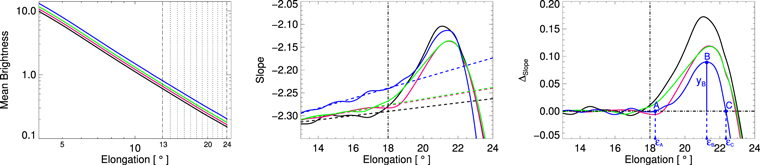
Figure 1. Left: Log–log representation of the mean brightness profile  (Δλ = 40°, 6+ years) for λ = 120° (black), λ = 170° (red), λ = 220° (green), and λ = 270° (blue). Center:
  (for short:
  ), same color code, elongation range restricted to 13° ≤
  ≤ 24°. The dashed-straight lines depict the robust linear fitting to
  in 13° ≤ ≤ 18° extrapolated to = 24°. Right: Difference between
  and the respective model (
 , same color code). The letters mark the relevant features for the analysis.
Download figure:
Standard image High-resolution imageIn the middle panel of Figure 1 we plot, with the same color code, the derivative of the sampled profiles  as shown in the left-hand panel (i.e.,
  to keep the notation simple, hereafter
  ) in the restricted elongation range 13° ≤ ≤ 24°. The curves show two distinct regions, namely (1) 13° ≤ ≲ 18°, and (2) ≳ 18°. For the profiles that are sampled, we see that
  follows a rather linear trend in the region 13° ≤ ≲ 18°. The dashed-straight lines depict the robust linear fitting to the corresponding smoothed measurements in this region, which are extrapolated to the end of the elongation range covered by ST-A/HI-1. A similar linear trend was observed in the derivative of each mean radial profile, independent of the S/C location. Therefore, we assumed that a linear model is a good option to represent its evolution in this elongation range.
The evolution of  in the outermost region (i.e., for ≳ 18°) is characterized by a well-defined, distinctive, bell-shaped pattern. Our working hypothesis is that the radial density distribution of the zodiacal dust cloud (which we assume can be described by the gradual, monotonic evolution of a linear model akin to the one that we derived in Stenborg et al. 2018) is affected by the presence of a density enhancement with certain characteristics, which we seek to describe by analyzing the excess brightness manifested by the bell-shaped portion of the brightness gradient. Therefore, in the right-hand panel of Figure 1, we show, with the same color code, the difference between the sampled profiles
  and the respective linear models that we used as proxy to describe the radial dependence of the zodiacal light (ZL) brightness along its photometric axis (hereafter
  ). The points A, B, and C (depicted for the profile obtained from 270° ecliptic longitude, in blue color) mark the relevant features for the analysis, namely: (1) A points to the elongation angle A where
  starts to depart from the linear model, (2) B points to the peak of the bell-shaped feature, which occurs at B with an amplitude yB, and (3) C points to the elongation angle C where
  intersects the extrapolation of the linear model near the outer edge of the instrument's FOV.
At this point, it is important to keep in mind that the analysis is carried out in the log-brightness gradient space. Therefore, the existence of the bell-shaped feature points out the presence of a localized brightness enhancement close to the outer edge of the ST-A/HI-1 FOV, in particular (1) A corresponds to the elongation angle where the brightness enhancement becomes discernible over the brightness arising from the smooth component of the Zodiacal dust cloud; (2) B corresponds to the elongation angle where the derivative is an extreme and points to the location of an inflection point of the actual sunward side of the brightness enhancement (i.e., where the rate at which the brightness enhancement reaches a maximum); and (3) C marks the elongation angle where the brightness enhancement reaches a relative maximum. Given the closeness of C to the outer edge of the ST-A/HI-1 FOV, it is clear that the downhill part of the brightness enhancement falls beyond the edge of the instrument's FOV. In other words, the bell-shaped feature in the derivative space signals the existence of a brightness enhancement but it only allows us to characterize its sunward half.
3. Results
As mentioned in Section 2, we observed the presence of a bell-shaped feature on the radial gradient of each mean brightness profile; i.e., on each  , λ = 0°, 5°, 10° ... 360°. In the top left-hand panel of Figure 2, we show a map of
  as a function of elongation (x-axis) and ecliptic longitude λ of the ST-A S/C (y-axis; the data along the y-direction has been cubic-interpolated to fill up the 5° gap between the averaged observations). The observations obtained from a S/C location between about 0° and 90° helioecliptic longitude (HAE system) are affected by the transit of the Milky Way in the outer portion of the ST-A/HI-1 FOV (see Stenborg & Howard 2017b; Stenborg et al. 2018), and hence are discarded from analysis. The black dots along the left and right edges of the colored band mark the A and C locations; i.e., the elongations where the brightness enhancement (1) start to be discernible, and (2) reaches a maximum, respectively (see the right-hand panel of Figure 1). The green dots point to the location B of the maximum amplitude of the bell-shaped feature (i.e., the location of the inflection point of the sunward side of the brightness enhancement). The inset color bar indicates the color scale with reference to the intensities reflected in the map.
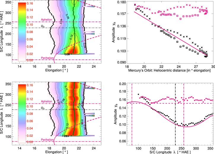
Figure 2. Excess brightness gradient  along the photometric axis. Top left: Azimuthal and radial dependence. The dashed line in red delineates the heliocentric distance rM of Mercury's orbit in units of degrees elongation. Top right: Log–log representation of the maximum amplitude of
  (i.e., intensity in the map on the top left-hand panel at the elongation of the green dots) as a function of rM (symbols in black). The red symbols depict the measurements de-trended by the linear model, as depicted in red. Bottom left: Same as top left-hand panel with the azimuthal dependence de-trended by rM(ϕ = 10°)−1.13. Bottom right: Maximum amplitude of (1)
  (in black) and (2) de-trended
  (in red). The red continuous line delineates the de-trending function rM(ϕ = 10°)−1.13. For details, see the text.
Download figure:
Standard image High-resolution imageThe map in the top left-hand panel of Figure 2 displays two peculiar features. Namely, the brightness enhancement (1) covers a projected radial region that roughly comprises the heliocentric distances covered by Mercury's present orbit (in Table 1 we show the orbital parameter of Mercury's orbit as computed for date 2011 January 1); and (2) extends along a full revolution around the Sun. The question that we look to answer in this work is whether this observational feature is a signature of a circumsolar dust enhancement near Mercury's orbit.
Table 1. Osculating Orbital Elements of Mercury with Respect to the Sun's Body Center (Epoch: 2011 January 1.0)
| Argument of perihelion | 291572 |
| Ascending node | 483164 |
| Inclination | 70043 |
| Eccentricity | 0.2056 |
| Perihelion distance | 0.3075 au |
| Aphelion distance | 0.4667 au |
| Orbital period | 87.9693 d |
Note. From JPL horizons online ephemeris system (https://ssd.jpl.nasa.gov/horizons.cgi#top).
Download table as: ASCIITypeset image
3.1. Role of Mercury
To help identify the location of the source that gives rise to the observed feature, the dashed-red line in the top left-hand panel of Figure 2 overplots the heliocentric distance rM of Mercury's orbit (epoch: 2011 January 1.0) at the corresponding longitude λ of the ST-A S/C (in units of elongation as measured from the average heliocentric distance of the observer). The ecliptic longitude of both the perihelion and the aphelion of Mercury's orbit in the time period studied is marked with the horizontal dashed–dotted lines in red (at about 77° and 257°, respectively). The descending node ΩD of the orbit is pointed out with the horizontal dashed–dotted line in black.
We notice in the map that, to first order, the amplitude of the bell-shaped feature in the radial gradients at B (green dots) seems to be inversely correlated with rM. To confirm this visual impression, in the top right-hand panel of Figure 2 we plot the maximum amplitude yB as a function of rM in a log–log representation. The crosses (squares) denote the yB measurements corresponding to observations from ecliptic longitudes that match those of the part of Mercury's orbit that recedes from (approaches) the Sun; i.e., from perihelion to aphelion (from aphelion to perihelion). We note that there exists a rather linear relation between the two variables, which is corroborated by the corresponding high absolute value of the Pearson correlation coefficient ρ. Namely, for the data set considering (1) the whole longitude range: ρ1 = 0.97, (2) only the longitudes from Mercury's perihelion to aphelion: ρ2 = 0.99, and (3) only the longitudes from Mercury's aphelion to perihelion: ρ3 = 0.98. Therefore, we can confidently assert that the amplitude yB follows, to a first approximation, a power law (i.e.,  ).
).
Before addressing the determination of the exponent α, we must note in the plot on the top right-hand panel of Figure 2 that the two branches do not superpose perfectly onto each other. The reason for this behavior is mainly twofold: (1) the possible existence of a phase-shift ϕ between yB and rM, and (2) the presence of brightening clumps asymmetrically distributed along the azimuthal profile of yB. In the absence of the latter, the former would constrain the measurements to distribute along a curve similar to an ellipse of decreasing eccentricity the greater the phase shift. However, as we shall soon see, both effects are present. The calculation of the phase shift is therefore subject to much uncertainty.
In spite of the inherent difficulties, we can estimate the phase shift by comparing the measurements yB and  (with rM(ϕ) we denote Mercury's orbit displaced ϕ° in ecliptic longitude) against the S/C longitude λ for different combinations of α and ϕ values. In particular, if α were known, in the ideal case of no brightness inhomogeneities (clumps), then the ratio of both curves should amount to unity independently of ecliptic longitude if in phase (i.e., the robust fitting to the ratio of both quantities is 0). If a phase shift existed instead, then a trend in ecliptic longitude should be manifested (i.e., a slope different from 0). Unfortunately, α is not known. Therefore, to circumvent this issue, we devised an iterative procedure to estimate both parameters simultaneously, which we briefly describe next.
To estimate the phase shift, we first assume α = 1 and look for the ϕ value that minimizes the slope of the robust line fitting to the ratio  *
*  versus λ. The plot on the top right-hand panel of Figure 2 is repeated (not shown here) and a robust straight line is fitted. The resulting slope of this model (i.e., the exponent α sought) is used as the input for the next iteration, where we look again for the value of ϕ that minimizes the slope of the aforementioned ratio. The procedure is repeated until
  . After four iterations we found ϕ = 10°, which yields
  . The error reported for the exponent is the estimated 1σ of the coefficient. In the plot on the top right-hand panel of Figure 2, the red squares (and crosses) represent the data set scaled by the resulting linear model with α = 1.13 (continuous red line).
In the bottom left-hand panel of Figure 2 we show the result of normalizing the whole map by rM(ϕ = 10°)−1.13 (with rM in units of Mercury's perihelion distance). With the exception of a few small intensity inhomogeneities, we note that the azimuthal trend is practically entirely removed. To better appreciate the effect of the observed modulation, in the bottom right-hand panel of Figure 2 we plot with the black circles the evolution of yB with the ecliptic longitude of the observer (i.e., the intensity of the map in the top left-hand panel at the location of the green dots). The vertical dashed lines denote the longitudes of Mercury's perihelion and aphelion (in red) and the descending node (in black). To emphasize the association between yB and rM, we over-plot rM(ϕ = 10°)−1.13 appropriately scaled (red continuous line). The red circles show the amplitude of the bell-shaped feature scaled by rM(ϕ = 10°)−1.13, hereafter ynB, with the horizontal dashed-red line indicating the base level. This brief exercise shows that, notwithstanding the physical meaning of ϕ (see Section 3.1.2), there is a clear association between the pattern observed and Mercury's orbit. Moreover, the normalized measurements reveal a couple of relatively small bumps near 285° and 335°, a larger one centered at about 210°, and another large half-bump peaking at about 110°. The nature of these clumps will be addressed in Section 3.1.1 and in the references therein.
Another relevant feature observed in the maps shown in the left-hand panels of Figure 2 is the azimuthal dependence of the inner boundary eA of the enhancement (delineated by the black dots on the left side of the colored band). From the maps, we infer that the brightness enhancement appears to be discernible from the smooth component of the ZL at a mean elongation of 183 (σ = 03), although the exact location seems to be modulated by a couple of factors, namely (1) the heliocentric distance of Mercury's orbit rM (note the maximum/minimum excursion in elongation near the location of Mercury's aphelion/perihelion), and (2) something else (note, e.g., the excursion toward lower elongations at around 210°). The former, which is a large-scale modulation, appears to be in phase with the behavior of yB, while the latter (at a smaller scale) seems to have no correlation at all (its analysis is deferred to Section 3.2).
Meanwhile, the outer edge of the bell-shaped feature (c) falls at a 3σ resistant-mean elongation of 2281, exhibiting only a marginal modulation (σ = 002). This means that the circumsolar brightness enhancement peaks at about 2281 and, unlike its inner boundary, lies at a rather constant heliocentric distance from the Sun's center.
From both the analysis carried out so far and the striking association found between the heliocentric distance of Mercury's orbital path and the observed modulation of both the magnitude and inner boundary of the brightness enhancement, we are certain that the enhancement observed is not an artifact. Rather, the data suggests the existence of a circumsolar dust density enhancement embedded in the smooth Zodiacal dust cloud that (1) starts at about 183 elongation (although the exact starting elongation depends upon a couple of factors; see Sections 3.1.2, 3.2, and 4.1), (2) peaks at about 228 elongation, and (3) exhibits a mean half-width of about 45, assuming that the full mean radial extent of the brightness enhancement is symmetric around the average location of its maximum.
Before continuing the analysis, it is important to note that our measurements only sample the dust density enhancement along the direction of the photometric axis of the F-corona, which precludes an analysis of its latitudinal extent. Next, we will: (1) attempt to quantify the excess density that characterizes this discrete feature of the ZL (Section 3.1.1), and (2) address in more detail its azimuthal geometry (Section 3.1.2).
3.1.1. Characterization of the Circumsolar Dust Density Enhancement
To quantify the excess dust density responsible for the brightness enhancement inferred, we must first estimate the relative brightness increase with respect to the brightness of the smooth component of the Zodiacal dust cloud. To this aim, we simply integrated the brightness gradient depicted in the map in the top left-hand panel of Figure 2 between A and j (j = A... C) for each S/C location λ. In particular, at = C, we calculate the excess brightness at the elongation where the relative increase with respect to the ZL is maximum (i.e.,  for simplicity hereafter we refer to it simply as
  ).
).
In the left-hand panel of Figure 3, we show a map with the azimuthal distribution of the excess brightness expressed as the relative percentage increase as a function of the observer's longitude λ, with the heliocentric distance of Mercury's orbit over-plotted in red. The red dotted–dashed lines mark the longitudes of the perihelion and aphelion of Mercury's orbit, and the black dotted–dashed line marks its descending node. To highlight the modulation exhibited in close association with Mercury's orbit, we display the percentage relative brightness increase at the peak of the dust ring (i.e.,  ) in the right-hand panel of Figure 3 (black dots). We note that, as observed from the ecliptic plane at ∼0.96 au (i.e., the average ST-A S/C heliocentric distance), the relative brightness increase measured from the S/C location λ appears to be inversely correlated with Mercury's orbit, with its minimum practically at the aphelion of the orbit, which is in qualitative agreement with our findings in Section 3.1. To help visualize this association, we show in red rM(ϕ = 0°)−1.13 (appropriately scaled). However, the reader will notice that for yB, the association was with rM(ϕ =10°)−1.13, while for
  is with rM(ϕ = 0°)−1.13 (i.e., no apparent phase shift). We also note that the maximum excess brightness
  amounts to about 1.3%–2.5% of the ZL smooth component depending upon the observer's location.

Figure 3. Relative percentage brightness increase with respect to the brightness of the Zodiacal dust cloud. Left: Azimuthal and radial distribution. The black dots depict A and C, and the green dots B (see the right-hand panel of Figure 1). Right: Brightness percentage increase at C (black circles). The red continuous line delineates the de-trending function rM(ϕ = 0°)−1.13, and the red circles the de-trended measurements.
Download figure:
Standard image High-resolution imageTo stress the association between the azimuthal dependence of the circumsolar excess brightness and Mercury's orbit, we draw the attention of the reader to the red dots in the right-hand panel of Figure 3. The red dots depict the excess brightness  (black dots) scaled by rM(ϕ = 0°)−1.13 (with rM in units of Mercury's perihelion distance) at the corresponding observer's longitude (in the same fashion as was done for the plot in the bottom right-hand panel of Figure 2). The normalized data reveal a base level brightness increase of about 2% with the presence of several brightness inhomogeneities (bumps) in concordance with the clumps observed in the plot in the bottom right-hand panel of Figure 2, namely (1) a broad bump centered at ∼210°; (2) a small bump at ∼285°; (3) a relatively large-amplitude bump at ∼350°, and (4) a half-bump starting at ∼110°. Note that there is also a marginal (noisy) increase at about 250°. The analyses of these particular features are deferred to Sections 3.1.2, 3.2, and 4.1. Next, we will attempt to estimate the excess dust density needed to produce the observed (average) increase in the ZL brightness.
The white-light F-coronal brightness results from the integration along the LOS of the product of the dust density and a factor related to the efficiency of the scattering at each scattering angle. The latter is a complicated function of the dust particles' composition, size, and the physics of the scattering, all of which is included in the so-called empirical Volume Scattering Function (VSF; e.g., Lamy & Perrin 1986; Mann 1992). Therefore, it is difficult, if at all possible, to disentangle the fractional contribution of the dust distribution along the LOS. However, the restricted elongation range of the brightness enhancement along with the observational features just described facilitate the analysis and, under certain assumptions, allow us to: (1) constrain the excess density necessary to reproduce the observed excess brightness, and (2) elaborate on the geometry and localization of the circumsolar dust density enhancement.
The simple calculation carried out at the beginning of this section (as reflected in Figure 3) shows that the excess brightness enhancement  apparently caused by a circumsolar dust density enhancement near the orbit of Mercury is on the order of
  in average over the brightness of the smooth Zodiacal cloud. We note that in the case of a constant (relative) density increase along the LOS (i.e., an enhancement not restricted to a localized region but extended uniformly along the LOS), the following identity holds:
  (here, ρ denotes dust density) assuming that the scattering properties of the two populations are similar. However, in the case of a circumsolar dust ring (and in the absence of any other significant discrete density feature along the LOS), the excess brightness is only due to dust density along a limited portion of the integration path, which is particularly most significant when the LOS tangentially traverses the ring. In this case, if we denote by x the relative contribution to the observed brightness by the dust outside the ring (0 < x < 1) and we make the assumption that the density enhancement in the ring is constant, then we may write

where  is the average observed excess brightness along the LOS (as inferred from Figure 3), and ΔIring is the true excess brightness that we are interested in, assumed to be sourced entirely from the circumsolar ring. By dividing the above expression by
  , we obtain
  . Therefore, we find that the circumsolar density enhancement necessary to produce the observed excess brightness is on the order of
  .
.
To (1) constrain the value of x and hence estimate the peak average density of the dust ring relative to the dust cloud along its photometric axis, and (2) shed light into the origin of the features revealed in the normalized measurements of the excess brightness (red dots in Figure 3), we show in the left-hand panel of Figure 4 a polar representation of Mercury's orbit (in red) along with the average location and extent of the bell-shaped feature (in green). The concentric circles delineate constant heliocentric distances (corresponding to elongation angles of 10°, 20°, 30°, 40°, 50°, and 60°), and the straight continuous lines represent ecliptic longitudes as measured counterclockwise from the first point of Aries τ (spaced every 20°). The concentric circles depicted with dashed lines point out both the inner (∼0.07 au) and outer (∼0.4 au) edge of the ST-A/HI-1 FOV (the average ST-A S/C orbit is represented by the thick black circle at about 0.96 au). The dashed line in red delineates Mercury's line of nodes and the dotted–dashed line (also in red) outlines the helioecliptic orientation of the major axis of the orbit.
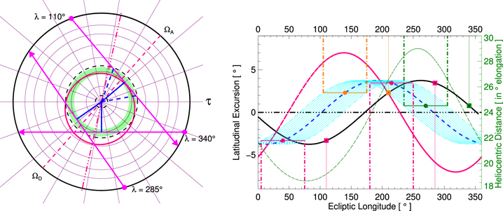
Figure 4. Mercury. Left: polar plot displaying Mercury's orbit in red. The intersection of the orbital plane with the ecliptic is delineated by the dashed line, and the orientation of the major axis by the dashed–dotted line. The three arrows mark three sampled LOS, and the blue segments their impact parameters. The green-shaded region displays the average location of the sunward-half portion of the brightness enhancement. The dashed circles in black show the extent of the FOV of the HI-1 instrument. The thick, black circle shows the average heliocentric distance of the ST-A S/C. Right: azimuthal evolution of the latitudinal excursion of the planet's orbit (in red), scale on the left axis. The colored squares mark the sampled LOS. The shaded light-blue region delineates the range where ∼50% of the brightness observed originates (for a LOS at ≈ 20°; see also the blue-dashed lines in the left-hand panel for LOS from λ ≈ 110°). The heliocentric distance of the the planet is depicted with the dashed-green line (scale on the right-hand axis).
Download figure:
Standard image High-resolution imageTo help explain the geometry of the dust ring, in the polar plot in Figure 4 we also draw the instrument's LOS at ≈ 20° from three selected S/C locations, namely at about λ = 110°, λ = 285°, and λ = 340° (i.e., the approximate ecliptic longitudes of the S/C where we noticed three of the brightness enhancements revealed in the normalized measurements in Figure 3). The thick lines in blue show the impact parameter of the respective LOS, which by construction fall at λ − (90° − ) ≈ λ − 70°. As shown in Sections 2 and 3.1.1, the excess brightness  is defined with respect to the brightness of the smooth component of the Zodiacal dust cloud. According to A. F. Thernisien (2018, private communication, in qualitative agreement with Misconi 1977) for an observer at 1 au, about 50% of the white-light F-coronal brightness at ≈ 20° arises from dust between about 0.7 au and 1.2 au from the observer (i.e., from a region along the LOS between ∼−35° and ∼37°, respectively, with respect to the impact parameter2
; see, e.g., the region delimited by the blue-dashed lines in the left-hand panel of Figure 4 for the LOS corresponding to λ = 110°). As noted in the polar plot, 50% of the integrated emission along the LOS at ≈ 20° arises from a region that traverses tangentially the dust ring. Therefore, we can estimate that (1 − x) ≈ 0.5. Based on this estimation of the relative contribution of the dust distribution along the LOS, the excess peak density Δρ/ρ necessary to produce the observed average peak excess brightness of 1.3%–2.5% (Figure 3) is on the order of about 3%–5%.
is defined with respect to the brightness of the smooth component of the Zodiacal dust cloud. According to A. F. Thernisien (2018, private communication, in qualitative agreement with Misconi 1977) for an observer at 1 au, about 50% of the white-light F-coronal brightness at ≈ 20° arises from dust between about 0.7 au and 1.2 au from the observer (i.e., from a region along the LOS between ∼−35° and ∼37°, respectively, with respect to the impact parameter2
; see, e.g., the region delimited by the blue-dashed lines in the left-hand panel of Figure 4 for the LOS corresponding to λ = 110°). As noted in the polar plot, 50% of the integrated emission along the LOS at ≈ 20° arises from a region that traverses tangentially the dust ring. Therefore, we can estimate that (1 − x) ≈ 0.5. Based on this estimation of the relative contribution of the dust distribution along the LOS, the excess peak density Δρ/ρ necessary to produce the observed average peak excess brightness of 1.3%–2.5% (Figure 3) is on the order of about 3%–5%.
3.1.2. On the Azimuthal Density Distribution of the Dust Ring
The evidence presented so far points toward the existence of a circumsolar dust ring that is characterized by a 3%–5% maximum excess density with respect to the background dust density, at a projected radial distance of about 0.38 au. The azimuthal modulation observed exhibits a clear dependence with the heliocentric distance rM of Mercury's orbit, in phase with the observer's longitude λ. However, in Section 3.1.1 we showed that, for a LOS at ≈ 20°, the bulk of the excess emission arises from ∼±35° from the longitude of the corresponding impact parameter; i.e., from ∼(λ − 70°) ± 35°. This apparent inconsistency is simply a result of the way that we computed the excess brightness. In particular, the null phase shift between rM and λ (i.e., the disassociation of the source location with respect to the observer) is simply due to the fact that the excess brightness is estimated from the difference of two periodic functions of rather comparable amplitude and phase. The reader is referred to the Appendix for a brief account of this fact.
Now we address the issue of the dust distribution along the ring. Figure 3 revealed the existence of four distinct brightness over-enhancements (Section 3.1.1). Our conjecture is that those features are signatures of density clumps that are embedded in the circumsolar dust ring. In particular, with the help of Figure 4 (left-hand panel) we see that the density clump that is inferred from the clump observed at λ ≈ 340° in Figure 3 seems to arise from a region close to Mercury's present orbit aphelion. Kuchner & Holman (2003) showed that dust particles in resonant orbits with small-mass planets in moderate eccentric orbits tend to accumulate at the apocenter of the planetary orbit, a finding that supports the interpretation of our observational result.
To help understand the origin of the other three over-enhancements and give more support to this interpretation, in the right-hand panel of Figure 4 we plot with the scale on the left axis the azimuthal dependence of the latitudinal excursion of: (1) the photometric axis of the F-corona in black (i.e., the elevation over the ecliptic where we sampled the density enhancement), and (2) the Mercury's present orbit in red. The dashed-blue line corresponds to the photometric axis shifted by δ = −(90° − ) ≈−70°, to show the ecliptic longitude of the impact parameter of the LOS at ≈ 20°; and the shaded, light-blue region delimits the ±∼35° range where 50% of the emission originates (see Section 3.1.1). The heliocentric distance of Mercury's orbit, also as a function of ecliptic longitude, is plotted in green with scale on the right axis. The colored squares point to the latitudinal excursion of the photometric axis at the S/C locations λ, where the over-enhancements in Figure 3 exist. The corresponding colored line segments, centered on the dashed-blue curve (marked with the colored circles) point to the approximate source region that is responsible for the corresponding over-enhancement.
Having set the framework, we can now proceed to analyze the source of each individual over-enhancement. The source of the feature at λ ≈ 340° (green square in the right-hand panel of Figure 4) originates along a region that comprises the ∼[235°–305°] ecliptic longitude range (green linear segment centered in the green circle); i.e., a region that fully encompasses the aphelion of Mercury's orbit. The feature at λ ≈ 285° (red square) is sourced between about 180° and 250° (red linear segment centered in the red circle at 215°). Interestingly, the LOS at the case elongation of ≈ 20° when the S/C is at λ ≈ 285° actually crosses Mercury's orbital path (notice the crossing of the red curve by the left branch of the corresponding linear segment). A similar argument is valid for the over-enhancement observed at λ ≈ 110°. As can be seen in the right-hand panel of Figure 4, there is no other case where Mercury's present path is actually crossed. Although two cases are not enough to give statistical significance to any interpretation, these last two cases seem to indicate that the dust ring would likely exhibit a maximum density along Mercury's orbital path.
As clearly shown in the right-hand panel of Figure 4, when the ST-A S/C is at λ ≈ 210° (orange square), the LOS at ≈ 20° falls away from Mercury's orbital path. Hence, the signature of the density clump recorded when the S/C is near this location seems to have no connection with Mercury. As we will see next (Section 3.2), an extra source of dust is required to explain it.
3.2. Role of Comet 2P/Encke
Narrow trails of dust along the orbits of short-period comets have been found in the IRAS data (Infrared Astronomical Satellite; Neugebauer et al. 1984), which were first reported by Sykes et al. (1986). In a later survey of IRAS data, Sykes & Walker (1992) detected eight dust trails associated with short-period comets and they concluded that dust trails are a characteristic feature of short-period comets. This finding was later confirmed by Reach et al. (2007) with a larger sample imaged with the 24 μm camera of the Spitzer telescope (Werner et al. 2004).
In a re-examination of COBE/DIRBE data (Hauser et al. 1998), Arendt (2014) found that the thermal emission of the dust trail of comet 2P/Encke (one of the eight short-period comets initially known to exhibit a dust trail, Sykes & Walker 1992) was the most obvious of the comet trails observed in the data. Since comet 2P/Encke crosses Mercury's orbit near its perihelion (the corresponding orbital parameters are reported in Table 2), and given the proven existence of an associated dust trail along its orbit (see also Reach et al. 2000; Gehrz et al. 2006), it is very likely that the dust ring observed in ST-A/HI-1 images might have a discrete contribution from comet 2P/Encke's trail.
Table 2. Osculating Orbital Elements of Comet 2P/Encke with Respect to Sun's Body Center (Epoch: 2011 January 1.0)
| Argument of perihelion | 18655021 |
| Ascending node | 3345667 |
| Inclination | 117823 |
| Eccentricity | 0.8483 |
| Perihelion distance | 0.3359 au |
| Period | 3.30 years |
Note. From JPL horizons online ephemeris system (https://ssd.jpl.nasa.gov/horizons.cgi#top).
Download table as: ASCIITypeset image
To examine this hypothesis, in the left-hand panel of Figure 5 we have duplicated the polar plot shown in the left-hand panel of Figure 4, with the orbit of comet 2P/Encke superposed in blue color along with the respective line of nodes and perihelion-aphelion line (depicted by the dashed and dotted–dashed lines, respectively). We note that the LOS at ≈ 20° for the observer's longitude λ ≈ 210° (depicted in pink) is very close to tangent to the orbit of the comet (the impact parameter of the corresponding LOS is at about 140°). At this longitude, 2P/Encke is in close proximity to Mercury's orbit. For a more comprehensive explanation we have also drawn in the polar plot (in orange) the LOS at ≈ 20° corresponding to λ ≈ 190° and λ ≈ 240°.

Figure 5. Comet 2P/Encke. Left: Mercury's and the comet's orbits (in red and blue, respectively) in a polar plot akin to that of Figure 4. The dashed–dotted (dashed) lines depict the perihelion-aphelion line (line of nodes) of the orbits (same color code). The three arrows mark three sampled LOS. The green-shaded region displays the average location of the sunward-half portion of the brightness enhancement. Right: azimuthal evolution of the latitudinal excursion of the comet's orbit (in blue and red) and of the photometric axis of the F-corona (in black), scale on the left axis. The colored squares mark the sampled LOS. The shaded light-blue region delineates the range where ∼50% of the brightness observed originates (for a LOS at ≈ 20°). The heliocentric distance of the comet is depicted with the dashed-green line (scale on the right axis).
Download figure:
Standard image High-resolution imageTo help visualize the effect of the comet's dust trail on the geometry of the dust ring in the ecliptic longitude range under discussion here (170° ≲ λ ≲ 240°, see Figure 3), in the right-hand panel of Figure 5 we depict a framework similar to that already set in Figure 4 (right-hand panel, see Section 3.1.2), where we replaced the orbital elements of Mercury by those of the comet 2P/Encke. Here, the blue curve delineates the latitudinal excursion of the orbital path of the comet (the portion in red highlights the part where the orbit falls within the FOV of the ST-A/HI-1 instrument; see the dashed-green line with scale on the right axis). The red squares points to the elevation of the photometric axis at the peak of the over-enhancement and the red segment centered on the red circle points to the approximate source region for a LOS at ≈ 20°. Likewise, the features in orange represent the setting for two sampled longitudes of the broad peak centered at λ ≈ 210° in Figure 3. In the plot, we see that at λ ≈ 210° the LOS crosses the orbital path of the comet almost exactly at its center. Moreover, the orange linear segments explain the broad aspect of the over-enhancement. For instance, at λ ≈ 240° the LOS just skims the comet's orbit, gradually increasing toward λ ≈ 210° to decrease afterward.
In Figure 6, we reproduce the map shown in the left-hand panel of Figure 3, this time as a function of the longitude of the impact parameter of a LOS at ≈ 20°. Superposed to the map, we plot with the dashed-blue line the 2P/Encke's heliocentric distance; the black-dashed line at ∼120° marks the longitude where Encke's and Mercury's orbits exhibit the same latitudinal excursion, and the dotted–dashed lines the nodes of Mercury' (in red) and 2P/Encke's (in blue) orbits. We notice in the map a bulge at the inner edge of the brightening enhancement (i.e., A), that peaks (i.e., exhibits the innermost excursion in elongation) very near 140° ecliptic longitude, i.e., where the LOS intersect the orbital path (marked by the straight blue-dashed line in the right-hand panel of Figure 5).

Figure 6. Azimuthal dependence of the brightness enhancement along the photometric axis of the F-corona. The dashed line in red delineates Mercury's orbit, the orbital nodes being pointed out by the dashed–dotted lines (also in red). The corresponding lines in blue depict the orbit of comet 2P/Encke and its descending node. The dashed line in black marks the longitude where Mercury's and comet 2P/Encke's orbit have the same latitudinal excursion.
Download figure:
Standard image High-resolution imageThe clear association between the location of the signatures observed and Encke's corresponding portion of the orbit indicates that the brightness enhancement observed at the S/C longitude λ ≈ 210° is due to a density clump that results from the dust trail along Encke's orbit. This statement is further reinforced by the finding of Killen & Hahn (2015) (see also Christou et al. 2015), who found that the dust trail along comet Encke's orbit is needed to explain the periodic variation of Mercury's calcium exosphere (Burger et al. 2014).
4. Discussion
Our observational findings point to the existence of a circumsolar resonant dust ring near Mercury's orbit. The ring appears to be azimuthally asymmetric, the density peak along the ring occurring at a projected radial distance of about 0.38 au. The peak excess density is of the order of about 3% to 5% above that of the smooth component of the Zodiacal dust cloud. Its sunward half-portion manifests a radial average (full) extent of about 45 (∼0.075 au), starting at about 0.3 au with a slight modulation in association with Mercury's orbital path and the perihelion of comet 2P/Encke. However, because our analysis was constrained to the radial direction along the photometric axis, we are unable to elaborate on its orientation. Moreover, at any given ecliptic longitude, the photometric axis scarcely samples the cross-section of the circumsolar ring, which, in particular, precludes a comprehensive analysis of the latitudinal fall-out of its density distribution.
The azimuthal distribution of the dust particles in the ring shows at least two distinct components, namely (1) dust particles belonging to the dust trail of comet 2P/Encke, which are constrained to ecliptic longitudes between about 100° and 170°, and (2) dust particles in apparent orbital resonance with Mercury (the component that gives origin to the ring). Given the characteristics of our observations, we are unable to elaborate on the source of the latter and hence it is beyond the scope of this paper to elaborate on theoretical aspects. Moreover, to increase the S/N of the brightness profiles along the photometric axes, we had to group them in longitude (40° bins) and time (6+ years). Therefore, any particular feature of the likely orbital resonances between the dust particles and Mercury is washed out and therefore precluded from identification (e.g., detection of dust trailing or preceding the actual location of the planet, or of the potential presence of dust gaps near the actual location of the planet, etc.). However, we did find an over-excess density near the aphelion of Mercury's orbit in qualitative agreement with theoretical modeling of resonant rings (e.g., Kuchner & Holman 2003).
These limitations of our approach rule out a full comparison of the properties of the circumsolar ring near Mercury's orbit with the other two known resonant dust rings in the inner solar system, namely the dust ring near Venus's (Jones et al. 2013, 2017), and Earth's (Reach 2010, and references therein) orbits. Unlike the dust ring near Earth (see Jackson & Zook 1989), the plausible existence of a dust ring near Mercury's orbit was never predicted theoretically nor even considered by modelers. Reach (2010) found that the Earth's circumsolar dust ring starts at 0.1 au from Earth, is centered 0.2 au behind Earth, exhibits a width of about 0.08 au along Earth's orbit, and is azimuthally asymmetric, as predicted by models for the evolution of dust spiraling inward under the influence of Poynting–Robertson drag; the latter being a property of resonant rings that was also observed in our measurements. Jones et al. (2013) found that the ring near Venus' orbit is double-peaked, with an average density increase over that of the smooth Zodiacal dust cloud of about 10%, compared to about 16% and 3%–5% for the rings near Earth's (Kelsall et al. 1998) and Mercury's orbits (this work), respectively.
4.1. Effect of Excess Dust Density Near the Observer
A close inspection of Figure 3 reveals that near λ ≈ 250° and λ ≈ 310°, the de-trended excess brightness measurements (red circles) are noisier and slightly above the basal level, respectively. The question that we seek to answer here is whether they point to some particular physical feature. Therefore, to look for a plausible cause for this (apparently marginal) behavior, we examined the possibility of brightness contamination due to dust near the observer's location. Even a small amount of excess dust density near the observer may produce a noticeable brightness increase as a result of the much higher efficiency of forward scattering at small scattering angles (e.g., van de Hulst 1947; Lamy & Perrin 1986).
As we have seen in Section 3.2, a plausible reason for a localized brightness over-increase is the crossing of the LOS rather tangentially to the dust trail of a short-period comet. Therefore, we first looked for short-period comets whose orbits cross the ST-A S/C orbit near the ecliptic plane. Comet 73P/Schwassmann–Wachmann 3 (hereafter SW3) has confirmed signatures of a dust trail along its orbit (see, e.g., Sykes & Walker 1992; Vaubaillon & Reach 2010; Arendt 2014). Its orbital parameters are reported in Table 3. We note that: (1) its descending node is at about 2498 (at this longitude the heliocentric distance of the orbit is 0.964 au); and (2) its perihelion distance is ∼0.94 au and occurs when the STEREO-A S/C is at λ ≈ 269°. Consequently, we considered it to be a suitable candidate to explain the noisier aspect of the excess brightness observed at λ ≈ 250°. In the left-hand panel of Figure 7 we have plotted in a polar graph the portion of the comet's orbit (in green color) in the surroundings of the ST-A S/C orbit (in black color). In the middle panel we plot: (1) its latitudinal excursion with respect to the ecliptic plane (pink circles, scale on the left axis), and (2) its heliocentric distance (dashed-green line, scale on the right axis). The dark green line on top the pink circles marks the latitudinal excursion of the comet when it is inside the ST-A S/C orbit (depicted by the black dashed–dotted line).
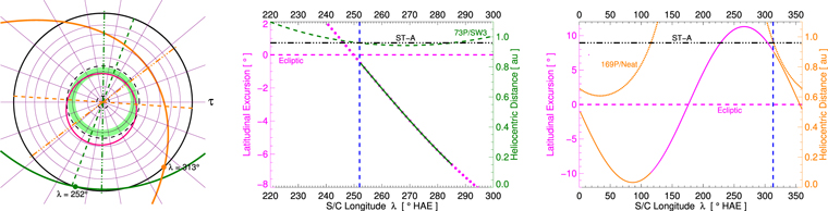
Figure 7. Dust trails local to the ST-A S/C. Left: orbit of comets 73P/Schawassmann–Wachmann 3 (SW3, in green) and 169P/NEAT (in orange) in a polar plot akin to those in Figures 4 and 5. The dashed–dotted (dashed) lines depict the perihelion-aphelion line (line of nodes) of the orbits (same color code). The azimuthal evolution of the latitudinal excursion (heliocentric distance) of the comets' orbits are detailed in the middle (SW3) and right (169P/NEAT) panels with scale on the left (right) axis. For further details, see the text.
Download figure:
Standard image High-resolution imageTable 3. Osculating Orbital Elements of Comets 73P/Schwassmann–Wachmann and 169P/NEAT with Respect to the Sun's Body Center (Epoch: 2011 January 1.0)
| 73P/Schwassmann–Wachmann | 169P/NEAT | |
|---|---|---|
| Argument of perihelion | 1988637 |
2179759 |
| Ascending Node | 698491 |
1761806 |
| Inclination | 113794 |
113016 |
| Eccentricity | 0.6923 | 0.7669 |
| Perihelion distance | 0.9425 au | 0.6077 au |
| Period | 5.36 year | 4.20 year |
Note. From JPL horizons online ephemeris system (https://ssd.jpl.nasa.gov/horizons.cgi#top).
Download table as: ASCIITypeset image
Comet 169P/NEAT is a plausible candidate to explain the feature at λ ≈ 310° (its orbital parameters are also reported in Table 3). The existence of a dust trail along the orbital path of this comet was first reported by Arendt (2014) after a re-examination of DIRBE data. Comet 169P/NEAT crosses ST-A S/C orbit path at about 116° and 313° ecliptic longitude (−98 and 77 from the ecliptic plane, respectively). The portion of the orbit of interest for the present analysis is over-plotted in orange in the left-hand panel of Figure 7. In the right-hand panel of Figure 7, we plot its latitudinal excursion with respect to the ecliptic plane (continuous orange and pink line, scale on the left axis; the portion in orange marks the part inside the ST-A S/C orbit). The comet's heliocentric distance is delineated by the orange circles with the scale on the right axis (the black dashed–dotted line marks the average S/C heliocentric distance).
If ST-A S/C indeed crosses an excess density region, then we should expect an overall increase of the brightness regardless of the elongation of the LOS. This will likely affect the gradient along the photometric axis and hence will be reflected in the mean value of the background models. In Figure 8, we plotted the azimuthal distribution of the value of the background models yM evaluated at the central elongation of the restricted elongation range (13° < < 18°) used to create them; i.e., yM( = 155) as a function of the mean S/C longitude λ (in black). The broad peak centered near 245° is due to brightness contamination associated with the passage of the back part of the Milky Way across the ST-A/HI-1 FOV. We also notice in the plot that there is a broad, albeit much smaller, bulge at around 310°. The wide aspect of the two bulges is either due to the extent of the physical feature responsible for the observed trait or an artifact resulting from the longitude range over which the observer's location was averaged for analysis (Δλ = 40°). To shed light into the nature of these effects, we repeated the analysis considering Δλ = 5°. The resulting mean value of the corresponding models is over-plotted in red in Figure 8. We notice (1) a sharp peak centered at 252° protruding from the wide bulge, and (2) a slightly wider but also sharp peak centered at 313°. The former is slightly asymmetric with respect to λ = 252°.
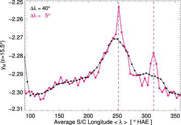
Figure 8. Azimuthal distribution of the linear model fitted to  in the restricted elongation range 13° < < 18° as evaluated at = 155; i.e., yM( = 155). Case study with Δλ = 40° in black and with Δλ = 5° in red. For further details, see the text.
Download figure:
Standard image High-resolution imageInterestingly, as we can see in the middle panel of Figure 7, at 252° (dashed-blue line), the comet SW3 is at about 0.96 au and very close to the ecliptic plane (about −04). Therefore, Figure 8 reveals that there is indeed a clear observable signature concomitant with the crossing of ST-A S/C through the orbital path of the comet. Moreover, for λ ≲ 250°, the evolution of the mean value of the background as computed with Δλ = 5° (red curve in Figure 8) matches the corresponding evolution as computed with Δλ = 40° (black curve), as expected (at these longitude ranges, the comet's orbital path lies outside the ST-A S/C orbit). However, for λ > 252°, the mean value falls more abruptly, in a clearly distinct fashion, to become negligible at about 270° (at this longitude, the comet is about −4° from the ecliptic plane; see the middle panel of Figure 7).
At λ ≈ 313° (see the right-hand panel of Figure 7, dashed-blue line), ST-A starts crossing the orbital path of comet 169P/NEAT, the comet's orbit being at about 77 above the ecliptic. Unlike the previous case, ST-A would just be skimming the dust trail here, hence the smaller effect observed in the plot of Figure 8 at λ = 313°. Meanwhile, at λ ≈ 116°, the comet's orbital path lies at about −10° degrees from the ecliptic plane. The lack of a noticeable well-defined feature in the mean value of the models at this ecliptic longitude suggests that the cross-section of the dust trail is not big enough to affect the observations.
In summary, the evidence presented here (although circumstantial) indicates that
(1) the noisier aspect of the normalized excess brightness measurements (Figure 3, red circles) observed near λ ≈ 250° seems to be the result of the combined outcome of the contaminating effect of both the Milky Way and the passage of ST-A through the orbital path of comet SW3 while within 4° from the ecliptic plane; and
(2) the normalized excess brightness measurements at λ ≈ 310° observed to be slightly above the basal level in Figure 3 is very likely a result of a contamination by dust local to the observer resulting from the crossing of ST-A through the outermost section of the dust trail of comet 169P/NEAT.
5. Summary and Conclusions
In this work, we have analyzed the photometric axis of white-light F-corona models constructed from ST-A/HI-1 images obtained during time period between 2007 December and 2014 March with a technique that was conceived to exploit the unique viewpoint of the upcoming Parker Solar Probe mission. In particular, we have shown that a numerical differentiation of the radial brightness gradient can reveal subtle stationary brightness increases in ST-A/HI1 data products on the order of 2%, occurring along projected heliocentric distances on the order of 0.1 au.
A thorough analysis has allowed us to identify the source(s) of the very faint brightness increase along the photometric axis of the F-corona models starting at about 18° elongation (∼0.31 au). In particular, the clear association found between the azimuthal dependence of the excess brightness and heliocentric distance of Mercury's orbit indicates that the excess brightness is a signature of a circumsolar (resonant) dust density enhancement in the neighborhood of the orbit of Mercury. Although the existence of such resonant rings have been simulated in deep detail, the density enhancement associated with Mercury's orbit has not been theoretically predicted, presumably because of the low mass of the planet and its closeness to the Sun. In other words, if the existence of the planet Mercury were unknown, then the observational evidence presented in this work would have suggested to us that a planet at about 0.4 au from the Sun should exist.
Moreover, a couple of extremely subtle brightness variations (<0.5%) embedded within the brightness signature of the ring could be singled out and their origin explained. We found them to be associated with: (1) the dust trail of comet 2P/Encke, and (2) the postulated existence of density clumps near the aphelion of the orbit of a low mass planet in an orbit of moderate eccentricity (Mercury in our case).
The approach that we have implemented also allowed us to find signatures of the crossing of the ST-A S/C through the dust trail of two short-period comets at about 0.96 au, namely 73P/Schwassmann–Wachmann 3 and 169P/NEAT.
In summary, this work has shown that, in spite of the known limitations of white-light observations to infer the properties of the dust grains, under certain circumstances it is possible to distinguish the sources of discrete excess brightness signatures. In particular, this led us to unearth the existence of a circumsolar dust ring near Mercury's orbit.
The SECCHI data are courtesy of STEREO and the SECCHI consortium. The STEREO/SECCHI data are produced by a consortium of NRL (USA), LMSAL (USA), NASA/GSFC (USA), RAL (UK), UBHAM (UK), MPS (Germany), CSL (Belgium), IOTA (France), and IAS (France). We acknowledge the support from the NASA STEREO/SECCHI (NNG17PP27I), SOC/SoloHI (NNG09EK11I) and the NASA/SPP/WISPR (NNG11EK11I) programs, and the support of the Office of Naval Research. We are grateful to Paul Landini (summer student under the 2016 Naval Research Enterprise Internship Program, NREIP), for his help in processing the STEREO/HI-1 background models.
Appendix: On the Origin of the Null Phase between Mercury's Orbit and the Observer's Longitude
In Section 3.1, we found that yB varies proportionally to rM−α(ϕ = 10°). However, according to the viewing geometry (Section 3.1.1), for = B it should vary accordingly to rM−α(ϕ = λ − δ), where δ ≈ 90° − B. To understand the origin of this apparent phase-shift discrepancy, we note that yB is the difference of two periodic functions, i.e., y( = B) and yM( = B). In particular, from this argument it is easy to see that  . Correspondingly, it is likely that the value of yM( = B) also contains a similar dependence on rM, either due to a real influence of Mercury or through an unforeseen bias in the linear model, albeit a potential small phase-shift Δϕ due to the different viewing geometry utilized to create the model (the background model was created by restricting the viewing elongations to 13° < < 18°). Therefore, under (1) the observational fact that the amplitude of these two functions does not differ much (<10%; see, e.g., the middle panel of Figures 1) and (2) the assumption that they both have a similar azimuthal dependence with a plausible, small phase-shift Δϕ, we can write (using Fourier expansion):
where Aj ≈ Bj (here, we have ignored the constant term of the expansion for simplicity). By combining these two expansions term-wise, we have

where

and

Note that here, we used the two-argument syntax for the arctangent, i.e., ψ = arctan(x, y), which is defined such that tan(ψ) = y/x while avoiding the 180° ambiguity in the standard (one-argument, i.e., arctan(y/x)) definition of the arctangent function. For a description of the differences between the one- and two-argument arctangent functions in IDL, the reader is referred to https://www.harrisgeospatial.com/docs/ATAN.html.
Equation (2) shows us that the precise phase of yB of each term of the expansion (i.e., ψj) only depends on the relative amplitudes and phases of y and yM. In other words, the explicit term δ ≈ 90° − B shift due to the viewing geometry has vanished, which is in agreement with our findings in Section 3.1. Since we assumed that the amplitudes Aj and Bj are similar, we expect ψj ≈ k, where k is a constant (in Section 3.1 we established that k ≈ 10°). In the following, we refer to k as the "net" phase.
In Section 3.1.1, we integrated  (i.e., y − yM) to obtain the radial profile of the excess brightness. In particular, at = C we found that the phase-shift ϕ between the resulting
  and rM was simply 0°. The particular net phase differences between the Fourier expansions of both the model yM and y( = j) with j = A...C will differ depending on elongation. Therefore, at each elongation comprised by the integrand,
  will exhibit a somewhat different net phase kj. Upon integration, they will combine into a net global phase, which does not necessarily have to match with the value k found at = C. In particular, we found the net global phase to be 0°.
Footnotes
- 2
![$\alpha =a\tan \left[\tfrac{d-\cos (\epsilon )}{\sin (\epsilon )}\right]$](data:image/png;base64,iVBORw0KGgoAAAANSUhEUgAAAAEAAAABCAQAAAC1HAwCAAAAC0lEQVR42mNkYAAAAAYAAjCB0C8AAAAASUVORK5CYII=) , with d = [0.7, 1.2] au, = 20°.
, with d = [0.7, 1.2] au, = 20°.
![$\alpha =a\tan \left[\tfrac{d-\cos (\epsilon )}{\sin (\epsilon )}\right]$](https://content.cld.iop.org/journals/0004-637X/868/1/74/revision1/apjaae6cbieqn43.gif)