


Abstract
The Carrington storm (1859 September 1/2) is one of the largest magnetic storms ever observed, and it caused global auroral displays in low-latitude areas, together with a series of multiple magnetic storms from 1859 August 28 to September 4. In this study, we revisit contemporary auroral observation records to extract information on their elevation angle, color, and direction to investigate this stormy interval in detail. We first examine the equatorward boundary of the "auroral emission with multiple colors" based on descriptions of elevation angle and color. We find that their locations were 36 5 ILAT on August 28/29 and 327 ILAT on September 1/2, suggesting that trapped electrons moved to, at least, L ∼ 1.55 and L ∼ 1.41, respectively. The equatorward boundary of "purely red emission" was likely located at 308 ILAT on September 1/2. If the "purely red emission" was a stable auroral red arc, it would suggest that trapped protons moved to, at least, L ∼ 1.36. This reconstruction with observed auroral emission regions provides conservative estimations of magnetic storm intensities. We compare the auroral records with magnetic observations. We confirm that multiple magnetic storms occurred during this stormy interval, and that the equatorward expansion of the auroral oval is consistent with the timing of magnetic disturbances. It is possible that the August 28/29 interplanetary coronal mass ejections (ICMEs) cleared out the interplanetary medium, making the ICME for the Carrington storm on September 1/2 more geoeffective.
Export citation and abstract BibTeX RIS
1. Introduction
It is known that extreme interplanetary coronal mass ejections (ICMEs) released from sunspots can cause severe magnetic storms, especially when they have southward magnetic fields (e.g., Tsurutani et al. 1992, 2008; Gonzalez et al. 1994; Willis & Stephenson 2001; Willis et al. 2005; Daglis et al. 1999; Daglis 2000, 2004; Daglis & Akasofu 2004; Echer et al. 2008a; Vaquero et al. 2008; Vaquero & Vázquez 2009; Schrijver et al. 2012; Odenwald 2015; Lakhina & Tsurutani 2016; Lockwood et al. 2016; Hayakawa et al. 2017a; Usoskin 2017; Takahashi & Shibata 2017; Riley et al. 2018). During magnetic storms, the horizontal component of geomagnetic fields decreases at low and middle latitudes (Gonzalez & Tsurutani 1987; Gonzalez et al. 1994; Daglis et al. 1999). Among the magnetic observations over approximately the past 1.5 centuries, the largest magnetic storm ever observed is considered to be the Carrington storm in 1859 (Chapman & Bartels 1940; Jones 1955; Chapman 1957; Mayaud 1980; Tsurutani et al. 2003; Cliver & Svalgaard 2004; Lakhina & Tsurutani 2016, 2017). Recent studies suggest evidence of several intense magnetic storms in the coverage of magnetic observations such as those in 1872 (Silverman 1995, 2006, 2008; Silverman & Cliver 2001; Vaquero et al. 2008; Cliver & Dietrich 2013; Cid et al. 2014; Viljanen et al. 2014; Lefèvre et al. 2016; Saiz et al. 2016; Lakhina & Tsurutani 2017; Hayakawa et al. 2018a, 2018c; Knipp et al. 2018; Love 2018; Riley et al. 2018), satellite observations of a near-miss extreme ICME in 2012 (Baker et al. 2013; Liu et al. 2014), and historical evidence before the coverage of magnetic observations (Willis et al. 1996; Ebihara et al. 2017; Hayakawa et al. 2016b, 2017a, 2017b, 2017c, 2018d).
On 1859 September 1, Carrington (1859) and Hodgson (1859) witnessed a white light flare as large as 2300 to ∼3000 msh (millionths of solar hemisphere; e.g., Cliver & Keer 2012; Hayakawa et al. 2016a) within a sunspot group, just before the maximum of solar cycle 10 in 1860 (Clette et al. 2014; Clette & Lefèvre 2016; Svalgaard & Schatten 2016). This flare is estimated to be X45 ±5 in terms of SXR class based on the amplitude of magnetic crochet and considered one of the most extreme flares in observational history (Boteler 2006; Cliver & Dietrich 2013). The following day (September 1/2), the ICMEs released from this active region brought intense magnetic storms with a maximum negative intensity of ∼1600 nT at Colaba (Tsurutani et al. 2003; Nevanlinna 2004, 2006, 2008; Viljanen et al. 2014; Kumar et al. 2015; Lakhina & Tsurutani 2016, 2017). Great auroral displays in low-latitude areas were reported at observation sites down to 22°–23° magnetic latitude (hereafter MLAT), as shown in Figure 1 (Kimball 1960; Tsurutani et al. 2003; Cliver & Svalgaard 2004; Cliver & Dietrich 2013; Hayakawa et al. 2016a; Lakhina & Tsurutani 2016, 2017). In addition to this storm, multiple magnetic storms occurred during the interval between 1859 August 28 and September 4 (Kimball 1960; Green et al. 2006; Green & Boardsen 2006; Hayakawa et al. 2016a; Lakhina & Tsurutani 2017), resulting from multiple flarings from the solar active region that could produce the multiple ICMEs and multiple sheaths, as is usually the case with extreme events (Willis et al. 1996, 2005; Mannucci et al. 2005; Tsurutani et al. 2007, 2008; Cliver & Dietrich 2013; Hayakawa et al. 2017a; Lakhina & Tsurutani 2017).
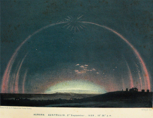
Figure 1. Drawing of an auroral display with a corona at Melbourne Flagstaff Observatory (S37°49', E145°09'; −47.3° MLAT) at 22:26 on 1859 September 2, reproduced from Neumeyer (1864). Neumeyer (1864, p. 242) describes this auroral observation as follows: "At 10.26 p.m. the light of stars of the third and fourth magnitude very much enfeebled. Beautiful rays through "Pisces". During the last 10 or 15 minutes a beautiful red arc of light, extending from E. to W., and passing through the crown, had become almost stationary. It followed the astronomical equator to a height of 70° where it deviated toward south." This drawing is reproduced in Cliver & Keer (2012) as well.
Download figure:
Standard image High-resolution imageThe auroral records during this stormy interval were also surveyed and rediscovered after Kimball (1960). So far, records such as those in U.S. ship logs (Green et al. 2006; Green & Boardsen 2006), American newspapers (Odenwald 2007), Australian reports (Humble 2006), Spanish newspapers (Farrona et al. 2011), historical documents in East Asia (Willis et al. 2007; Hayakawa et al. 2016a), and Mexican newspapers (Gonzalez-Esparza & Cuevas-Cardona 2018) have been surveyed. These rediscovered records have provided further insights into the auroral displays during this stormy interval.
These magnetic storms caused one of the earliest space weather disasters or space storms (see also Daglis 2003 for the terminology) such as disturbance in the telegraph system (e.g., Loomis 1861b, 1865). Boteler (2006) and Muller (2014) summarized glitches of telegraph transmissions and showed that telegraph operations were disrupted in North America and Europe on August 28/29 and September 1/2–2/3. Due to the increasing dependence upon the electricity and electronics, our society becomes increasingly vulnerable to the space weather disasters or space storms (Daglis 2000, 2004; Baker et al. 2008). Had it occurred in the present time, the consequences are thought to be disastrous for a modern civilization that depends on electronic devices, although this detail is still controversial (Baker et al. 2008; Hapgood 2011, 2012; Calisto et al. 2013; Cannon et al. 2013; Oughton et al. 2016; Dyer et al. 2018; Riley et al. 2018). Therefore, research on such extreme magnetic storms is important in geophysics and solar physics, as well as in various other scientific fields (e.g., Schwenn 2006). In this context, how frequently such extreme magnetic storms occur has also been discussed (e.g., Willis et al. 1997; Love 2012; Riley 2012; Schrijver et al. 2012; Yermolaev et al. 2013; Cliver & Dietrich 2013; Shibata et al. 2013; Usoskin & Kovaltsov 2012; Maehara et al. 2015; Curto et al. 2016; Riley & Love 2017), although the methodologies and predictions vary from each other.
It is known that the auroral oval moves equatorward, and the aurorae dominated by red color appear in middle- and low-latitude areas during magnetic storms (Tinsley et al. 1986; Shiokawa et al. 2005). The magnetic latitude of the equatorward boundary of the auroral oval is correlated with the disturbance storm-time (Dst) index (Yokoyama et al. 1998). The Dst index is used as a measure of the magnetic disturbance. Thus, the equatorward boundary of the auroral emission region may be used as a proxy measure for a magnetic storm when geomagnetic field data are unavailable. Note that further rediscovery of auroral records in lower magnetic latitudes can always update this estimation. To minimize the uncertainty, we prefer to determine the equatorward boundary of the auroral emission region, rather than determining the equatorward boundary of auroral visibility.
The equatorward boundary of auroral visibility during the interval between 1859 August 28 and September 4 has been thoroughly studied, but their exact values remain somewhat controversial (e.g., Kimball 1960; Tsurutani et al. 2003; Green & Boardsen 2006; Cliver & Dietrich 2013). On the one hand, Kimball (1960) states that red glows were visible down to 22° to 23° MLAT on September 1/2, and this was adopted by Tsurutani et al. (2003). On the other hand, Green & Boardsen (2006) concluded that the aurorae were visible as low as ∼18° MLAT on September 2/3, and ∼25° MLAT on 1859 August 28/29.
As for the equatorward boundary of the auroral emission region, Kimball (1960; see Figure 6) considered that "overhead aurorae" were coming down to 34°–35° MLAT, while the "southern extent of visibility" went down to 22°–23° MLAT in the eastern United States on 1859 September 1/2. Considering that the equatorward boundary of the auroral oval is a better measure than the equatorward boundary of auroral visibility to scale magnetic storms (Yokoyama et al. 1998), we believe that reevaluating the equatorward boundary of the auroral emission region is important to scale the magnetic storms in the stormy interval around the Carrington storm more precisely.
It should also be noted that stable auroral red arcs (SAR arcs) are frequently visible as reddish glows a few degrees equatorward of the auroral oval (Rees & Roble 1975). SAR arcs are typically observed during the storm recovery phases (Shiokawa et al. 2005) and are thought to coincide with the interaction region between the plasmapause and the inner edge of the ion plasma sheet (or the ring current; Cornwall et al. 1970, 1971; Kozyra et al. 1997). Therefore, the equatorward boundary of the SAR arc may provide a rough estimate of the inner edge of the ion plasma sheet (or the ring current). Tsurutani et al. (2003) assumed that the purely red emission corresponds to SAR arcs and estimated the inner edge of the ring current. Using the location of the ring current, Tsurutani et al. (2003) estimated the magnetospheric electric field and used this value to obtain the Dst value for the Carrington storm. Hereinafter, we use the term "auroral emission region" instead of "auroral oval" because we cannot exclude the possibility of SAR arcs.
In the reevaluation of the equatorward boundary of the auroral emission region, there are some difficulties as follows. First, the majority of previous studies have only considered the magnetic latitude of observational sites and have not considered the auroral elevation angle therein. We need to consider the elevation angle of the auroral display in eyewitness reports in low magnetic latitude to reconstruct the equatorward boundary of the auroral emission region. Second, the exact locations of the equatorwardmost observational sites of Green & Boardsen (2006) are not very clear. Green & Boardsen (2006) seem to rely on the equatorwardmost observations written in the ship deck log in NARA, as shown in their Table 1 and Figures 1 and 2. Table 1 dates the observations from Panama 1859 August 29, while Figures 1 and 2 place the observations from Panama on "September 2–3." On the contrary, Green et al. (2006) show that all of these records are dated 1859 August 28/29. Third, a difficulty also arises from the fact that the auroral emission extends roughly 100–400 km along a magnetic field line that is highly inclined at low magnetic latitudes. In this paper, we reevaluate the equatorward boundary of the auroral emission region during this stormy interval from 1859 August 28 to September 4 on the basis of eyewitness reports of auroral displays with their elevation angle, color, and brightness, according to historical documents from that time.
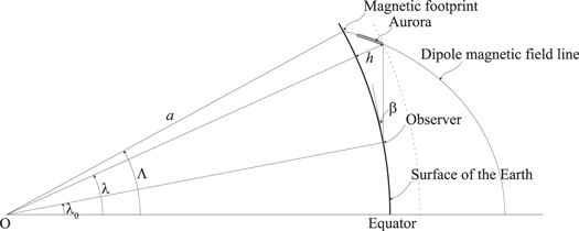
Figure 2. Relationship between the elevation angle of the auroral display, β, and the invariant latitude of the aurora, Λ, in dipole geometry.
Download figure:
Standard image High-resolution image2. Materials and Methods
In order to visit the magnetic storms that occurred between 1859 August 28 and September 4, we examine contemporary source documents for eyewitness auroral reports (see the references in Appendix A) from low-latitude areas (<35° MLAT). The first document is the contemporary auroral reports compiled by Loomis, which primarily cover the western hemisphere and were once cataloged by Kimball (1960). After the intense auroral display in 1859, Loomis called for eyewitness reports from the readers of the American Journal for Science to collect worldwide auroral reports from the western hemisphere. The second document contains the auroral reports from U.S. Navy ship logs. This record group was introduced by Green & Boardsen (2006) and Green et al. (2006) and formed the backbone of their discussion. The third is the historical documents in East Asia that were introduced by Hayakawa et al. (2016a), with one more record that was found after its publication (HJ5). As contemporary East Asian residents did not understand the physical nature of auroral displays, these records are not found in scientific accounts, but rather in the diaries or chronicles from these countries (see Hayakawa et al. 2016a). The fourth is the reports in Mexican newspapers, recently rediscovered by Gonzalez-Esparza & Cuevas-Cardona (2018).
We analyze this extreme auroral display in the Carrington storm based on its elevation angle, color, and brightness, as well as based on eyewitness reports with dates from low-latitude areas (<35° MLAT) in these contemporary source documents. We first compute the magnetic latitude of the observation sites. We define the magnetic latitude as the angular distance from the dipole axis. The dipole axis is determined by using the geomagnetic field model GUFM1 (Jackson et al. 2000). When the geographical coordinates of observational site are not given in original documents, we estimate the location of observational sites as the old town/city areas in given sites, unless otherwise endorsed, considering the development of town/city area in mid 19th century (e.g., Ezcurra & Mazari-Hiriart 1996). In this process, we revised some of the geographical coordinates of Kimball (1960) and Gonzalez-Esparza & Cuevas-Cardona (2018). Especially, we found the observational sites reported by Gonzalez-Esparza & Cuevas-Cardona (2018) are somewhat located westward from the known old town/city area by 6 ∼ 80 km. For example, Gonzalez-Esparza & Cuevas-Cardona (2018) located Mexico City as the geographical coordinate as "19.39 (latitude) and −99.28 (longitude)" corresponding to the location of current San Fernando District, while the Mexico City had not expanded enough to cover this district in mid 19th century, as seen in Figure 2 of Ezcurra & Mazari-Hiriart (1996). Therefore, we revised the geographic coordinates of observational sites so as to correspond to the old town, unless otherwise endorsed. Note that we have not included the report of Michoacán and San Luis Potosí in Gonzalez-Esparza & Cuevas-Cardona (2018), as they are without the exact date in their source document. Likewise, we have not included the report of Montería in Columbia in 1859 (Moreno Cárdenas et al. 2016), as this report was originally dated as "Marzo (March)" without exact date in 1859 and its dating is not clear (Exbrayat 1971, p.151).
We then extract information on elevation angle, color, and brightness from the original eyewitness reports. We use the information on elevation angle of auroral display to determine the equatorward auroral extension by geometric calculation. We then analyze the distribution of auroral color to determine what kind of elements were influenced by incident electron particles, and finally apply the simulation code by Ebihara et al. (2017) to reconstruct the auroral brightness during this magnetic storm. Finally, we compare their duration with contemporary magnetic observations taken from the Colaba Observatory in India (Moos 1910a, 1910b; Tsurutani et al. 2003; Kumar et al. 2015) and magnetic observatories from the contemporary Russian Empire (e.g., Nevanlinna 2004, 2006, 2008).
3. Equatorward Extensions of the Auroral Emission Region and Visibility between 1859 August 28 and September 4
3.1. Estimation of the Equatorward Boundary of the Auroral Emission Region
After assembling the eyewitness reports from Loomis's collection, U.S. Navy ship logs, East Asian historical documents, and Mexican newspapers we extract observation sites with the lowest magnetic latitudes (<35° MLAT). To estimate the equatorward boundary of the auroral emission region, we need information on the elevation angles in these reports. The "overhead aurora" as presented in Figure 6 of Kimball (1960) can be regarded to have the elevation angle of 90°. We should note that the instantaneous distribution of auroral displays depends on time and magnetic local times. It is our intention to find the most-equatorward extension of the auroral emission region, not to find the spatiotemporal evolution of the auroral emission region.
During this stormy interval, 13 records are found to contain information about the elevation angle of the aurora as listed in Table 1. Assuming the height of the upper border of the aurora, we estimate the equatorward boundary of the auroral emission region on the basis of the geometry of the dipole magnetic field line as shown in Figure 2 (see also Hayakawa et al. 2018b). We also assume that (1) the aurora is very thin in the latitudinal direction and is extended along a dipole magnetic field line, and that (2) atmospheric refraction is negligible. The magnetic latitude of the aurora λ at height h can be computed using the following equation for a given elevation angle β and magnetic latitude of the observation site λ0:

where a is Earth's radius. With the dipole magnetic field, we can compute the magnetic latitude of the magnetic footprint of the aurora Λ as

Λ is referred to as an invariant latitude (ILAT), which is associated with the L-value (≡1/cos2 Λ). Hereafter, we evaluate the equatorward boundary of the auroral emission region in terms of ILAT.
In reality, the aurora has finite thickness. When the observer is located equatorward of the aurora (Λ > λ0), the top border of the aurora provides an estimate of the equatorward boundary of the aurora regardless of the latitudinal thickness of the aurora.
The altitude of the upper border of the aurora is problematic because the volume emission rate of the aurora gradually decreases with altitude, and there is no clear border. According to Monte Carlo simulations, the peak altitude of the volume emission rate at 630.0 nm [O i] is ∼350 km and ∼270 km for the precipitating electrons with monochromatic energy of 100 eV and 500 eV, respectively (Onda & Itikawa 1995). Of course, the simulation result depends on the energy and pitch angle distributions of the precipitating electrons as well as the temperature of electrons, ions, and neutrals, and their atmospheric constitution (Solomon et al. 1988). The precise altitude of the volume emission rate is not our focus because the description of the aurora has no precise information about the altitude distribution of the brightness. In reality, the distribution function of the precipitating electrons is not monochromatic, and the altitude profile of the volume emission rate depends on the distribution function of the precipitating electrons. Ebihara et al. (2017) surveyed the distribution function of the precipitating electrons measured by the DMSP satellites for severe magnetic storms and identified two components of the distribution function. One component peaks at ∼70 eV and the other one peaks at ∼3 keV. According to the two-stream electron transport code used by Ebihara et al. (2017), the volume emission rate at 630.0 nm peaks at ∼270 km for the electron distribution function measured in the severe storms. The altitude at one-tenth of the maximum volume emission rate occurs at ∼410 km altitude.
3.2. Auroral Display during August 28/29
Table 1 and Figure 3(a) summarize the observation sites at magnetic latitude less than 35° on August 28/29. During these days, the equatorwardmost site of auroral visibility is 202 MLAT (Panama; Saranac, 1859 August 29), while Green & Boardsen (2006) concluded that the equatorward boundary of this auroral visibility is 25° MLAT. Note that Green & Boardsen (2006) dated the record at Panama August 29 in their Table 1, while they dated it September 2/3, not August 28/29, in their Figures 1 and 2.
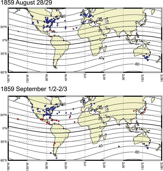
Figure 3. Observational sites of auroral displays during 1859 August 28/29 (a: top) and September 1/2 (b: bottom). Only the sites within ±60° are shown. The sites with magnetic latitude lower than 35° are shown in red (see Table 1). The sites with magnetic latitude higher than 35° are shown in blue. The latter observational sites are based on reports by Loomis (L1-L8), WAMG (Heis 1859, 1860), Neumeyer (1864), and references and data reductions in Humble (2006), Green & Boardsen (2006), and Farrona et al. (2011). The observational report of Honolulu is shown in the lower panel for reference. The contour indicates the magnetic latitudes in 1859 calculated on the basis of the GUFM1 magnetic field model.
Download figure:
Standard image High-resolution imageAt the same time, Fritz (1873) mentioned that the aurora was visible at St. George del Mina, the current El Mina (N05°05', W001°21'), on 1859 August 28. If this were the case, the aurora would have been visible down to 99 MLAT according to the GUFM1 model (Jackson et al. 2000). However, the original text shows that it was Dr. Daniels who wrote "from St. George del Mina (West Coast of Africa)" who witnessed the auroral display "at 19°50' west of Greenwich and 28° north" (WAMG, v.3, p.38 = WA2)." Therefore, his observation (WA2) took place not at St. George del Mina (N05°05', W001°21'; 99 MLAT), but at the sea near Cabo Verde (N28°, W19°50'; 355 MLAT), as also suggested by Silverman (2008). Therefore, the equatorwardmost observational site (visibility) on August 28/29 should be located at Panama (202 MLAT).
Nevertheless, it does not necessarily mean that the equatorward boundary of the auroral emission region came to the zenith of Panama. The record of Saranac at Panama (202 MLAT) does not provide information about the elevation angle of this auroral display a little before 04:00 LT. However, we find the auroral display "rising to the zenith" at Havana (340 MLAT) around 04:00–04:10 LT on August 29 (L1, pp. 403–404 = L1-8). If we simply assume that the upper border of the aurora is at 400 km altitude, we can estimate the equatorward boundary of the auroral emission region to be 365 ILAT (or 340 MLAT at 400 km altitude). In this case, the auroral display can be seen up to an elevation angle of 7° at Panama (202 MLAT).
3.3. Auroral Display during September 1/2–2/3
Table 1 and Figure 3(b) summarize the observation sites at magnetic latitude less than 35° during September 1/2–2/3. On September 1–2, the two most-equatorward sites are −218 MLAT (Valparaiso, Chile; L4, p. 399 = L4-15) and 228 MLAT (at sea; L6, p. 361 = L6-2-43, and WAMG, v.3, p.270 = WA1). We excluded the record at Honolulu because the exact date of the auroral observation is not provided in the original document (L5, p. 88). We must also note that another cluster of observation sites is found in East Asia down to 231 MLAT (Shingu, Japan).
The most-equatorward report having information about elevation angle comes from Sabine (231 MLAT). The record of Sabine is not included in Kimball (1960), but is consistent with his result in terms of the latitudinal extent of auroral visibility. The report from Sabine shows that the auroral display extended up to 35° in elevation angle from 00:30 LT to 01:30 LT on September 2 (Sabine, 1859 September 02). Assuming the auroral height of ∼400 km and substituting the β of 35° and λ0 of 231 into Equations (1) and (2), we estimate the equatorward boundary of the auroral emission region to be 308 ILAT (or 277 MLAT at 400 km altitude). Likewise, another naval record by Captain Kraan (WA1) shows that a reddish aurora was visible up to 30° in elevation at sea (N14°28', W024°20') and lets us estimate the equatorward boundary of the auroral emission region to be 313 ILAT (or 282 MLAT at 400 km altitude) between 4:30 LT and 5:15 LT on September 2. These records are consistent with the record at Porto Rico (298 MLAT), in which "luminous rays, red, purple and violet, extended even to the zenith" (L5, p. 88 = L5-14) almost simultaneously (at ∼07 UT on 1859 September 2) and that at Havana (340 MLAT), "which passed the zenith toward the northeast, attaining the height of 100°, accompanied with whitish rays and also with the red rays, more vivid then the general tones of the segment rising to the zenith, yet without passing it" (L1, p. 405 = L1-8). Based on these reports, the equatorward boundary of the auroral emission region is estimated to be 327 ILAT and 354 ILAT, respectively.
Recently recovered Mexican reports also support this estimation. Reports from Mexico City (MX1, 288 MLAT), Querétaro (MX2, 298 MLAT), and Zimapán (MX4, 301 MLAT) show that the auroral displays reached the zenith and suggest that the equatorward boundary of the auroral emission region came down to 318 ILAT, 327 ILAT, and 319 ILAT, respectively. The report from Zimapán is interesting as it may possibly refer to auroral corona, mentioning "a silver lily in the shape of an arc of a great circle" from the region where "glowing rays extended downwards as if to meet a red light that shone up from the northern horizon" (MX4; see also Gonzalez-Esparza & Cuevas-Cardona 2018).
If the historical description in Honolulu (205 MLAT), in which the aurora extended up to 35° from the horizon, mentions the aurora found on September 1/2, the auroral oval during this interval would be extended to 285 ILAT (or 251 MLAT at 400 km altitude). In short, these remote and independent observation sites of low-latitude aurorae suggest the following:
- 1.The most-equatorward magnetic latitudes (MLATs) of the auroral visibility are ∼202 during the August 28/29 storm, and −218 and 228 during the September 1–2 storm.
- 2.The most-equatorward invariant latitudes (ILATs) of the auroral emission region are 365 during the August 28/29 storm, and 308 during the September 1/2 storm.
These latitudes are lower than those estimated by Kimball (1960). Moreover, the equatorward boundary of the auroral emission region during the September 1/2 storm, obtained here, lets us compare this event with another rivaling extreme event on 1872 February 4 (Chapman & Bartels 1940; Chapman 1957; Cliver & Svalgaard 2004; Tsurutani et al. 2005; Silverman 2008). During this storm, an aurora was observed at Bombay (100 MLAT), as Chapman & Bartels (1940) noted (Tsurutani et al. 2005; Silverman 2008). Recent surveys in the East Asian sector showed that the aurora was observed at the zenith of Shanghai (199 MLAT), with the equatorward boundary of the auroral emission region reconstructed as 242 ILAT, and estimated that the auroral display would have been indeed visible at Bombay within the elevation angle of 10°–15° (Hayakawa et al. 2018a). Further studies are needed to compare these extreme space weather events suggested by Chapman (1957).
4. Color of the Auroral Display
As shown in Table 1, the auroral display during the stormy interval basically shows red color, but some of them show other colors. For example, on August 28–29, whitish auroral displays were observed at Havana as well (340 MLAT) in the northern hemisphere (L1, pp. 403–404). On September 1/2, the observer at Porto Rico (298 MLAT) noticed "luminous rays, red, purple and violet, extended even to the zenith" (L5, p. 88), and another observer at Guadeloupe (275 MLAT) "noticed two rays of whitish light which rose parallel to each other, passing a little to the left of the pole star" (L3, p. 265). In the southern hemisphere, an observer at Santiago noted, "brilliantly illuminated by a light, composed of blue, red, and yellow colors, which remained visible for about three hours" at 02:00 LT on 1859 September 2 (L4, p.399).
These colorful auroral displays including the whitish one may suggest the existence of greenish aurorae (557.7 nm [O i]) and/or bluish aurorae (427.8 nm [N+]) caused by the precipitation of electrons with energy above ∼1 keV, in addition to the above-mentioned red aurorae. The mixture of these auroral displays may explain the whitish and yellowish aurorae as well. A similar description is found in the much earlier historical document for auroral displays in 771/772 and 773, with rays or scepters in colors of "blood-red, green, and saffron-colored" observed at Amida (45° MLAT) according to the Zūqnı̄n Chronicle (MS Vat. Sir. 162, f.150v, f.155v; Hayakawa et al. 2017b). The cause of the precipitation of the electrons remains an open question.
The appearance of rays with whitish, red, purple, and violet colors may result from a fold in a sheet-like structure of aurora (Oguti 1975). When the sheet-like structure of the aurora is folded, the line-of-sight integral of the light is increased, resulting in a localized enhancement of brightness at all wavelengths. If this is the case, the formation of a sheet-like aurora in the low-latitude aurora dominated by a red color would be a problem because such a sheet-like red-dominated aurora is unusual. If the rays were caused by a localized enhancement of electron precipitation, magnetospheric processes would be a problem because localized precipitation of low-energy electrons is unusual at low latitudes. Anyway, the records in Table 1 raise a new problem regarding low-latitude aurora. The deep inner magnetosphere (L < 1.5) may be much more complicated than we believe.
Most of the records in Table 1 indicate that the aurora is dominated by red color (most likely 630.0 nm [O i]). With optical measurements with a bandpass filter, Miyaoka et al. (1990) and Shiokawa et al. (2005) have shown that there are two types of red display observed in Japan. One is the red-dominant display with emission at 557.7 nm (e.g., 1989 October 21 and 2003 October 29–30). The energy source for the red-dominant display is the precipitation of low-energy electrons (<∼100 eV; Banks et al. 1974). The precipitating electrons excite the atomic oxygen to the O(1D) state, and the transition O i (3P–1D) results in emission at 630.0 nm (Rees & Roble 1975). The transition O i (1D–1S) gives rise to emission at 557.7 nm. The excitation energies of the O i(1S) and O(1D) states are 4.19 and 1.97 eV, respectively (Rees & Roble 1975). The emission at 630.0 nm dominates that at 557.7 nm because the probability of the O(1D) state is about 10 times higher than that of the O i(1S) state (Rees 1989). If this were the case, electrons would originate from adiabatically accelerated plasmaspheric populations (Ebihara et al. 2017). The other type is the red display without discernible emission at 557.7 nm (e.g., 2000 April 7). This can be regarded as an SAR arc (Roach & Roach 1963). The energy source of the SAR arc is heated electrons (∼3000 K) associated with heat flows from high altitude or very low-energy particle flux (Cole 1965; Cornwall et al. 1970, 1971; Kozyra et al. 1997). The thermal electron flux decreases with energy, which also gives rise to the dominance of 630.0 nm (Kozyra et al. 1997). Very bright SAR arcs with intensity up to 13 kR were observed when a large magnetic storm occurs (Baumgardner et al. 2008). There are at least three processes for the energy conversion from magnetospheric ions to ionospheric electrons (Kozyra et al. 1997), including Coulomb collision (Cole 1965), wave–particle interaction (Cornwall et al. 1971), and kinetic Alfvén waves (Hasegawa & Mima 1978). If this were the case, the red-dominant display corresponds to the footprint of the interaction region between the storm-time ring current and the plasmasphere. Mendillo et al. (2016) showed an example where the red aurora (∼200 km altitude) and the SAR arc (∼400 km altitude) coexist on the same field line. It should be noted that Tsurutani et al. (2003) used the equatorward visibility (∼23° MLAT) of these "red glows" in Kimball (1960) to scale this magnetic storm in comparison with the magnetic observation at Colaba.
It is not straightforward to distinguish between the aurora and the SAR arcs from the existing records, due to the lack of objective records from scientific equipment. Considering formless features and the red-dominated color of SAR arcs with relatively longer durations (Cornwall et al. 1970, 1971; Kozyra et al. 1997), one may consider the red-dominated displays without other colors or motions and with longer duration at low magnetic latitude to be SAR arcs (K. Shiokawa 2018, private communication). Forms are not a good criterion for distinguishing them because structured SAR arcs are observed (Mendillo et al. 2016). As listed in Table 1, some records fit these criteria at, for example, La Union (L3-31, 238 MLAT), Kingston (L3-29, 291 MLAT), and Montego Bay (L3-29, 295 MLAT). These are likely to be SAR arcs because the reddish aurora had been observed without motion for ∼4–5 hr. With information about the elevation angle at La Union (L3-31, 238 MLAT), we estimated that the equatorward boundary of the aurora extended to 322 ILAT. The most-equatorward boundary of the aurora with a red color only was located down to 308 ILAT (at Sabine, RG24-2). They are also presumably considered as SAR arcs, unless some typical motions or structures are otherwise mentioned.
At the same time, there are some auroral reports that are unlike SAR arcs even down to the lowest magnetic latitude; these are possibly related to auroras by broadband electrons (e.g., Shiokawa et al. 1997, 1999). Auroras with multiple colors are reported down to 298 MLAT with "red, purple, and violet" colors (Porto Rico) and −221 MLAT with "blue, red, and yellow colors" (Santiago, L4-15). The equatorward boundary of the auroral emission region with multiple colors is estimated to be 327 ILAT (Porto Rico, L5-14). They are not likely SAR arcs as they have non-reddish components. Likewise, a report at 205 MLAT (Honolulu) describes "Broad fiery streaks shot up into and played among the heavens" in it, although their dating is uncertain. This is likely the ray structure of type A aurorae (Chamberlain 1961), rather than SAR arcs. If we can date this record to September 1 as in Kimball (1960), the equatorward boundary of the auroral oval could be calculated even down to 285 ILAT, considering its elevation angle to be ∼35°. These reports show that not only SAR arcs but also usual auroras were distributed even down to the most-equatorward location in terms of their visibility.
The equatorward boundary of the auroral oval may provide the upper limit of the inner edge of the electron plasma sheet (e.g., Vasyliunas 1970). Horwitz et al. (1982) showed two examples indicating that the equatorward boundary of the auroral oval coincides with the inner boundary of the plasma sheet and the plasmapause. On the other hand, the equatorward boundary of the SAR arcs may reflect the interaction region between the plasmasphere and the inner boundary of the ion plasma sheet (or the storm-time ring current; Cornwall et al. 1970, 1971; Kozyra et al. 1997). The Earthward transport of the electron plasma sheet and the ion plasma sheet is most likely caused by the enhancement of the large-scale convection electric field. The magnetospheric convection is enhanced when the southward component of the interplanetary magnetic field (IMF) arrives at Earth (e.g., Kokubun 1972).
The strong convection electric field transports fresh electrons originating in the nightside plasma sheet toward Earth through the E × B drift. When the electrons experience pitch angle scattering, some of them are scattered into the loss cone, resulting in the diffuse aurora (e.g., Lui et al. 1977). The equatorward boundary of the (diffuse) aurora is reasonably supposed to provide an upper limit to the Earthward boundary of the electron plasma sheet. The Earthward boundary of the electron plasma sheet is determined by the strength of the convection electric field, and is located at, or outside of, the plasmapause (Ejiri et al. 1980).
Fresh ions originating from the nightside plasma sheet are also transported Earthward as previously mentioned by Tsurutani et al. (2003) for the Carrington storm. Because of the energy-dependent drift velocity, the inner edge of the ion plasma sheet depends on the particle perpendicular kinetic energies. Observations have shown that ions at particular energies can penetrate into the plasmapause (Smith & Hoffman 1974). The energy-dependent penetration of ions is called a nose structure (Smith & Hoffman 1974) and is theoretically explained by Ejiri et al. (1980). When ions at particular energies interact with the plasmaspheric cold plasmas, the temperature of the plasmaspheric cold electrons increases. Consequently, the electron temperature increases in the topside ionosphere, causing the SAR arc emissions (Cornwall et al. 1970, 1971; Kozyra et al. 1997). We note that the inner edge of the ion plasma sheet may have some ambiguity of a few degrees in magnetic latitude because the equatorward boundaries of the ion plasma sheet depend on energy (Ejiri et al. 1980). The equatorward boundary of the SAR arc may provide a rough estimate of the inner edge of the plasma sheet, although it may have some ambiguity.
In general, the SAR arcs cannot be explicitly distinguished from the usual aurora caused by energetic electron precipitation without spectroscopic instruments. Miyaoka et al. (1990) presented a photograph of the low-latitude aurora dominated by red color. The picture shown by Miyaoka et al. (1990) looks like purely red aurora. However, according to data from a scanning photometer, the red-dominated aurora contains emission at 557.7 nm (green), which means that the red-dominated aurora is most likely an aurora, not an SAR arc. Thus, we cannot conclude, at the present stage, that all of the purely red emission found in the historical records correspond to the SAR arcs.
5. Abnormal Auroral Brightness during the Carrington Storm
Intense electron precipitation can cause much brighter aurorae than normally expected at low latitudes. The Baltimore American and Commercial Advertiser on 1859 September 3 (p. 2, col. 2) described the magnificent auroral display "on late Thursday night" (1859 September 1) and concluded that the auroral "light was greater than that of the moon at its full." Other similar descriptions are found in low-latitude areas (<35° MLAT), as summarized in Table 1. At Guadeloupe (275 MLAT), "its ruddy light was noticeable in the interior of the houses" (L3, p. 265). At La Union (238 MLAT), the auroral display was described as "light ... equal to that of day-break, but was not sufficient to eclipse the light of the stars" (L3, p. 265). At Concepcion (−255 MLAT), the auroral display "threw out some flame or vapor, and spread a light like that of the moon" (L4, pp. 398–399). Other records generally compare this auroral display with a conflagration or colossal fire, especially in East Asia (see Hayakawa et al. 2016a).
Based on the above-cited descriptions, we consider the auroral brightness to be Class IV International Brightness Coefficient (IBC), where the total illumination on the ground equals that of the full Moon (Chamberlain 1961). IBC Class IV is suggested to correspond to a brightness of approximately 1000 kR for the "green aurora" at 557.7 nm (Hunten et al. 1956). As far as we know, such bright aurorae have probably not been recorded by modern scientific instruments at low latitudes (Hikosaka 1958; Shiokawa et al. 2005). Similar bright aurorae, which are described "as bright as a night with full moon" at Nagoya, Japan (N35°11', E136°54', 252 MLAT; Ebihara et al. 2017), have been recorded in East Asia but in 1770, before magnetic observations. Unusually intense electron precipitation, about an order of magnitude larger than that observed in the 1989 March 14 storm, is expected to cause the bright aurorae corresponding to Class IV (Ebihara et al. 2017).
SAR arcs are observed to be as bright as 13 kR during the large magnetic storm (Baumgardner et al. 2008). If the purely red emission corresponds to an SAR arc, the brightness will be problematic. An extremely dense ion plasma sheet (or the ring current) and/or an extremely dense plasmaspheric electron population is expected to occur in 1859. This problem remains to be solved in future studies.
6. Geomagnetic Disturbances
6.1. General Overview
Figures 4 shows the duration of auroral observations together with records of observations at magnetic observatories in Helsinki (HEL: N60°10', E24°57'), St. Petersburg (STP: N59°56', E30°18'), Ekaterinburg (EKA: N56°49', E60°35'), Barnaul (BAR: N53°20', E83°57'), Nertchinsk (NER: N51°19', E119°36') (Nevanlinna 2006, 2008), and Colaba in India (Tsurutani et al. 2003; Kumar et al. 2015) for 1859 August 28–29 and September 2, respectively. We converted the observation time of each record from local time (LT) to universal time (UT), according to their longitude (see Humble 2006; Nevanlinna 2008). Unfortunately, the magnetic field at Colaba is missing during the interval from 11 UT on August 28 to 12 UT on August 29 because the Colaba magnetic observatory did not perform observations on Sundays and holidays during the period 1847–1872 (Moos 1910a, p. 105). At 12 UT on August 29, the deviation of the magnetic field (ΔH) is −484 nT, suggesting that a magnetic storm could have commenced during this missing interval. It is reasonable to consider that this stormy interval from 1859 August 28 to September 4 is composed of, at least, two magnetic storms probably caused by ICMEs from the same active region. A similar stormy interval was observed in 2003 October during which multiple ICMEs were launched from the same flaring active region (NOAA 10486) (Yashiro et al. 2004), causing successive large magnetic storms (Shiota & Kataoka 2016). In 2004 November, multiple ICMEs were also launched from the same active region (NOAA 10696), causing successive large magnetic storms (Echer et al. 2010). One single ICME is unlikely to cause successive magnetic storms with an interval of three to four days. One single ICME may cause the two-step development of magnetic storms (Kamide et al. 1998; Daglis 2004) when the southward component of the IMF is embedded both in the sheath and the magnetic cloud in the ICME (Tsurutani et al. 1988).

Figure 4. From top to bottom: magnetic disturbance in the H-component (magnetic north–south component) at Helsinki (HEL), St. Petersburg (STP), Ekaterinburg (EKA), Barnaul (BAR), and Nertchinsk (NER); magnetic component in the D-component (magnetic east–west component), magnetic disturbance in the horizontal component at Colaba, and time and magnetic latitude when the aurora was seen from 1859 August 28 to September 4 (UT). The horizontal (red) thick line indicates the possible equatorward boundary of the auroral emission region in ILAT estimated from the auroral elevation angle. The horizontal (black) thin line indicates the MLAT where the aurora was visible. The report from Honolulu is plotted assuming it was observed on September 1/2.
Download figure:
Standard image High-resolution imageIf multiple ICMEs launched from the same active region, the former one could be decelerated by momentum transfer or aerodynamic drag as it propagated into interplanetary space due to the "snow plow" effect (Tappin 2006; Takahashi & Shibata 2017). If the solar wind density is low on its trailing side, the latter ICME, leaving the Sun several days later, could proceed in interplanetary space without substantial deceleration, as the former one had cleared out the interplanetary mass in advance (Tsurutani & Lakhina 2014; Shiota & Kataoka 2016). Because of the lower "snow plow" effect, the latter one could have hit Earth's magnetosphere without substantial deceleration, becoming more geoeffective and resulting in the extreme storm on September 1/2, known as the Carrington storm. If this is the case, the former one could play an important role in causing the Carrington storm.
Carrington's sunspot observations seem to support this scenario. As reproduced in Figure 5, a large active region was already on the eastern hemisphere of the Sun on August 28 and arrived at the central meridian on September 1. Carrington noticed this active region on August 25 (C3, v.2, f.312a) and monitored it (C1, v.2, ff.63a-64a). During this observation, Carrington witnessed the white light flare on September 1, as published in Carrington (1859). In his original logbook, he highlighted the region with white light flares in reddish color (C1, v.2, f.64a). Cliver (2006) reviewed the flare on September 1 in more detail.

Figure 5. Carrington's sunspot drawings on August 28 and September 1, shown in projected images (see Plate 1 of Carrington 1863 and Figure 2 of Cliver & Keer 2012). The whole disk drawings on August 28 and September 1 are shown above (C3, v.2, ff.312a-313a). The relevant parts of his logbook on August 28 and September 1 are shown here (C1, v.2, ff.63a-64a). These manuscripts are currently preserved in the archive of the Royal Astronomical Society, as shown in Appendix A.6 (courtesy of the Royal Astronomical Society).
Download figure:
Standard image High-resolution imageTypically, the main phases of magnetic storms last at most a few hours in duration, in combination with sheaths and magnetic clouds (Tsurutani et al. 1988; Echer et al. 2008b), although the Hydro Quebec storm in 1989, an exception, was reported to last for up to a whole day (Allen et al. 1989). However, recent analyses clarified that multiple sheaths and magnetic clouds combined to cause this "storm" with an apparent long duration and classified this "storm" as a "compound magnetic storm" (Lakhina et al. 2013; Lakhina & Tsurutani 2017). Likewise, in the magnetic observation at Colaba, the main phase of the Carrington storm lasted at most ∼1.5 hr with a fast recovery phase within these storms. It was probably caused by the strong southward component of the IMF (Tsurutani et al. 2003, 2018). Compared with the "compound (multistep) magnetic storm" of 1989, Lakhina et al. (2012) and Lakhina & Tsurutani (2017) considered the Carrington storm a "one-step" storm, most probably caused by a magnetic cloud within the ICME (Kamide et al. 1998; Daglis 2004). Moreover, the one-step Carrington storm was one of many storms that occurred between August 28 and September 4, presumably caused by multiple ICMEs from the same active region (Cliver & Dietrich 2013).
6.2. Magnetic Observations during 1859 August 28/29
In Figure 4, the H-component of the magnetic field started to decrease at 23 UT on August 28 and recovered by 12 UT on August 29 (EKA, BAR, and NER). Thus, it is speculated that the magnetic storm of 1859 August 28/29 commenced at 23 UT on August 28. This period roughly corresponds to the period of the auroral display at Havana (340 MLAT) from 20:45 LT on August 28 to 04:20 LT on August 29 (from 0145 UT to 0920 UT on August 29) and two maritime observations. At 0400–0410 LT (1029–1039 UT), the aurora was "rising to the zenith" at Havana. Assuming that the topside border of the aurora was located at 400 km altitude, we estimate the equatorward boundary of the auroral oval to be 365 ILAT as indicated by the thick horizontal line in Figure 4. The aurora observed in Panama (202 MLAT) around 0300–0400 LT (0918–1018 UT) is indicated by the red horizontal line in Figure 4. As discussed above, the same aurora was visible in Panama and Havana. EKA, BAR, and NER were located on the dawnside. The negative excursion of the H-component is probably caused by the westward-flowing Hall current associated with the DP2 current system, i.e., the ionospheric convection. If this is the case, ionospheric convection would be enhanced during this period by the intense southward component of the IMF and fast solar wind. The enhanced convection electric field could result in the Earthward penetration of the magnetospheric plasma originating from the nightside magnetosphere. The Earthward electron penetration could result in the equatorward displacement of the auroral oval. Earthward penetration is accompanied by adiabatic acceleration of the plasma, resulting in enhanced plasma pressure in the inner magnetosphere, particularly in the ring current.
After the missing interval, the magnetic field observation at Colaba resumes at 12 UT on August 29 with a ΔH of −484 nT. After that, ΔH shows a gradual increase until ∼00 UT on August 31. The gradual increase probably indicates a remnant of the recovery of the storm that probably initiated at 23 UT on August 28 as speculated from the high latitude observation of the magnetic field. Because of the missing interval at Colaba on August 28 (Bombay Local Time), we cannot count the number of storms during this interval, or identify the minimum of the magnetic disturbance. It is considered multiple storms probably occurred during this interval as in the "compound storm" in 1989 (Lakhina et al. 2013; Lakhina & Tsurutani 2017), and these storms commenced at ∼23 UT on August 28, with the total duration of these storms as ∼49 hr.
6.3. Magnetic Observations during 1859 August 1/2–2/3
On 1859 September 1/2, there were pronounced large-amplitude, bipolar disturbances in the D-component at least at STP and NER, in addition to the disturbances in the H-component. The horizontal component of the magnetic field is largely depressed at Colaba at 06–08 UT on 1859 September 2. We propose two scenarios for the magnetic disturbances on 1859 September 1/2. The first scenario is based on the spatial variation. The downward field-aligned current (dawnside part of the Region 1 current; Iijima & Potemra 1976) located just equatorward of the observatories caused the eastward disturbance on the dawnside (e.g., STP and NER at 05–07 UT). The ionospheric Hall current flowing eastward caused the northward disturbance (e.g., STP and NER). This is consistent with the magnetic observations at Rome and Greenwich indicating that there was a strong westward Hall current associated with the convection (Boteler 2006). The amplitude of the positive excursion in the H-component at NER is smaller than that at STP because STP was probably close to the throat of the dayside convection. As Earth rotates, the observatories moved from the dawn sector to the dusk sector. The upward field-aligned current (duskside part of the Region 1 current) caused the westward disturbance on the duskside (e.g., NER). The ionospheric Hall current caused the southward disturbance (e.g., STP, BAR and NER). The second scenario is based on the spatial variation. The center of the downward field-aligned current moved rapidly equatorward of the observatories, and the downward current caused the eastward disturbance on the dawnside (e.g., STP and NER at 05–07 UT). Then, the upward field-aligned current moved poleward rapidly. The upward current located poleward of the observatories caused the westward disturbance (e.g., STP and NER at 07–09 UT).
At midday, the center of the Region 1 field-aligned current is located at 74°–77° ILAT for the magnetically quiet period (Iijima & Potemra 1976). During the intense magnetic storms, the center of the Region 1 field-aligned current expands to as low as 50–55° ILAT on the nightside (Fujii et al. 1992; Ebihara et al. 2005). Ngwira et al. (2014) performed a global magnetohydrodynamics (MHD) simulation for a Carrington-type event assuming extremely high densities of the ICME for this event, and showed that the center of the Region 1 field-aligned current is located between 40° ILAT and 50° ILAT during the main phase of the model storm on the dayside. The MHD simulation result is consistent with the variation of the D-component magnetic field on September 2–3. As for August 28–29, such bipolar variation is not clearly seen in the D-component. This probably indicates that the center of the Region 1 current was located well poleward of the observatories. Most of the auroral displays start to appear at the same time as the sharp magnetic disturbance.
For the interval from September 2 to 3, the auroral displays were continuously seen during the main and recovery phases of the magnetic storm. This can be explained as follows. Electrons are injected Earthward due to the enhanced magnetospheric convection (probably associated with the enhanced Region 1 field-aligned current). When the injected electrons are scattered by some processes into the loss cone, the aurora becomes illuminated. The seed electrons trapped in the inner magnetosphere could remain during the recovery phase, which caused the long-lasting auroral displays at low latitudes. Substorm-associated injection may also supply hot electrons deep into the inner magnetosphere. The substorm-associated injection is well observed at a geosynchronous orbit, whereas is not observed in the deep inner magnetosphere, such that L < 1.5, as far as we know.
The September 2/3 observations of the aurora at La Union and San Salvador are unusual as they are isolated to low-latitude auroral observations. While this may be due to the possible misdating of September 1 as considered by Kimball (1960), the record explicitly writes that it started "about 10 o'clock ...on the night of September 2d" (L3, p. 265), namely 04h UT on September 3 and corresponds to the recovery phase around this time (Nevanlinna 2006, Figure 4).
The H-component of the magnetic field recorded at Colaba shows a rapid recovery on September 2. Li et al. (2006) postulated an extremely high solar wind dynamic pressure enhancing the magnetopause current flowing in the eastward direction. One possibility is the strong magnetopause current that increases the H-component of the magnetic field. If the rapid recovery of the H-component of the magnetic field is attributed to the rapid decay of the ring current, there will be some mechanisms for this (Ebihara & Ejiri 2003), including charge exchange (Dessler & Parker 1959), resonant interaction with ion cyclotron waves (Cornwall et al. 1970; Tsurutani et al. 2018), replacement with tenuous plasma stored in the plasma sheet (Ebihara & Ejiri 1998), and pitch angle scattering of ions in a curved field line (Ebihara et al. 2011).
The first plausible mechanism for rapid decay is charge exchange. Using the neutral hydrogen (geocorona) density model of Rairden et al. (1986) and the cross-section model of Janev & Smith (1993), we can estimate the lifetime for the charge exchange between H+ with energy of 100 keV and H to be 8.5 hr at L = 1.5. The lifetime for the charge exchange between O+ with energy of 100 keV and H is 1.0 hr with the cross-section model of Phaneuf et al. (1987). Hamilton et al. (1988) suggested that the rapid recovery of the Dst index during a large magnetic storm (minimum Dst value of −306 nT) is caused by the rapid loss of O+, although Kozyra et al. (1998) raised a question about the capability for charge exchange in rapid loss. The second mechanism is the replacement of the ring current with a tenuous one (Ebihara & Ejiri 2003). During the main phase, a large number of ions are transported from the plasma sheet to the lower L-shells by the convection electric field. If the plasma sheet density decreases rapidly, the tenuous plasma is transported to lower L-shells, replacing the previously transported one with the freshly transported one. The energy density in the heart of the storm-time ring current decreases rapidly, and the total amount of the particles' energy decreases rapidly, which gives rise to the rapid decay of the ring current. This idea is tested by Keika et al. (2015). The third mechanism is resonant interaction with electromagnetic ion cyclotron waves for the rapid loss of the ring current ions (Tsurutani et al. 2018).
It is likely that an unusual loss process could occur during the Carrington storm because of the uniqueness of its nature. Careful diagnosis is still needed to account for the rapid recovery of the H-component of the magnetic field at Colaba. To better understand the rapid recovery, the equatorward boundary of the auroral emission region, as we have estimated in this paper, provides valuable information.
7. Conclusion
In this study, we revisited historical records in magnetically low-latitude areas less than 35° MLAT during the stormy interval between 1859 August 28 and September 4 including the Carrington storm on September 1/2. We revisited these records in the East Asian, South American, and North American sectors, and we extracted information on their elevation angle, color, direction, and duration. Some of the low-latitude auroral displays during this storm were reddish, suggesting possibilities of auroras and SAR arcs. However, the auroral displays were not only purely red. Some records include bluish, yellowish, and whitish colors. These historical records show us that the equatorward boundary of auroral emission with multiple colors during the Carrington storm was 365 ILAT on August 28/29 and 327 ILAT on September 1/2. This may correspond to the equatorward boundary of the auroral oval. The equatorward boundary of purely red emission was 308 ILAT on September 1/2. This may correspond to the SAR arcs. The SAR arcs cannot be explicitly distinguished from the usual aurora caused by energetic electron precipitation without spectroscopic instruments. In that sense, we cannot definitely conclude that all of the purely red emission correspond to SAR arcs. This reconstruction of the observed auroral emission region provides a conservative estimate of the intensity of the magnetic storm, and finding further auroral reports suggesting extension to lower magnetic latitudes could always improve this estimate. The brightness of these auroral displays was classified IBC Class IV. These facts suggest that high-energy electrons also precipitated, partly, in low-latitude areas during this stormy interval, in addition to the precipitation of low-energy electrons. Finally, we compared their duration with contemporary magnetic observations and confirmed that multiple magnetic storms occurred during this stormy interval, and that the equatorward expansion of the auroral oval is consistent with the timing of magnetic disturbances.
We acknowledge the Bilateral Joint Research Projects between Japan (JSPS) and India (DST), the Supporting Program "UCHUGAKU," Mission Research Projects of RISH (PI: H. Isobe), and SPIRITS 2017 (PI: Y. Kano) of Kyoto University. This work was also encouraged by a Grant-in-Aid from the Ministry of Education, Culture, Sports, Science and Technology of Japan, grant number JP15H05816 (PI: S. Yoden), JP15H03732 (PI: Y. Ebihara), JP16H03955 (PI: K. Shibata), JP15H05815 (PI: Y. Miyoshi), JP15K05038 (PI: M. Soma) and 18H01254 (PI: H. Isobe) and a Grant-in-Aid for JSPS Research Fellow JP17J06954 (PI: H. Hayakawa). We gratefully thank E. W. Cliver and K. Shibata for preliminary reviews and valuable comments on our manuscript, D. Shiota for fruitful discussion on the possible impact of successive ICMEs on Earth's magnetosphere, SILSO for providing data of sunspot number, UKSSDC for providing the data for magnetic storms and sunspot area, WDC Kyoto for providing the data for geomagnetism, National Astronomical Observatory of Japan and ISEE (Nagoya University) for their partial financial supports, the archivists in the Izawa Library for permission for the research of Chikusai Nikki, K. Shiokawa for his advice on SAR arcs, S. Prosser and the Royal Astronomical Society for providing the manuscripts by R. Carrington, J. M. Vaquero and J. Humble for advice and help on the original auroral records in Spain and Australia, and the National Archives and Records Administration for help with and permission for research.
Appendix A: References for Historical Documents
In Appendix A.1, we provide the references for the historical sources in Table 1. The abbreviations used in "Ref" show where these records are from: L (E. Loomis's publications in the American Journal of Science (AJS)), RG24 (Record Group 24 of the National Archives of the United States: Logs of the U. S. Naval Ships and Stations, 1801–1946), HC (Historical Records in China), HJ (Historical Records in Japan), and MX (Mexican Newspapers). When they are published in books, journal articles, or critical editions, we provide their publication name, volume, and page number. When they are unpublished manuscripts, we provide their title, volume, folio number, shelf mark, and name of holding archive in their original languages for traceability to original source documents. Note that full records of HC, HJ (except for HJ5), and MX have been transcribed and translated in Hayakawa et al. (2016a) and Gonzalez-Esparza & Cuevas-Cardona (2018).
Table 1. List of Observational Sites at Magnetic Latitude below 35° MLAT
| Ref | Year | Month | Day | Place | Latitude | Longitude | Start | End | Direction | Color | Elevation | MLAT | MLAT (EB) | ILAT (EB) |
|---|---|---|---|---|---|---|---|---|---|---|---|---|---|---|
| L1-8 | 1859 | 8 | 28 | Havana | N23°07' | W82°22' | 20:45 | 28:20 | N-Z | R/W | zenith | 34.0 | 34.0 | 36.5 |
| L7-4 | 1859 | 8 | 28 | At sea | N25°45' | W27°04' | 23:15 | midnight | NW | R | ⋯ | 34.4 | ⋯ | ⋯ |
| L3-27 | 1859 | 8 | 28 | Inagua | N21°18' | W73°04' | ⋯ | ⋯ | ⋯ | ⋯ | ⋯ | 32.6 | ⋯ | ⋯ |
| RG24-1 | 1859 | 8 | 28 | Panama | N08°59' | W79°31' | 27:00 | 28:00 | ⋯ | R | ⋯ | 20.2 | ⋯ | ⋯ |
| L3-28 | 1859 | 9 | 1 | Cohe | N20° | W76°10' | ⋯ | ⋯ | N | R | ⋯ | 31.5 | ⋯ | ⋯ |
| L3-29 | 1859 | 9 | 1 | Kingston | N17°58' | W76°48' | 25:00 | 29:00 | ⋯ | R | ⋯ | 29.1 | ⋯ | ⋯ |
| L3-29 | 1859 | 9 | 1 | Montego Bay | N18°21' | W77°56' | 22:00 | 29:00 | ⋯ | ⋯ | ⋯ | 29.5 | ⋯ | |
| L3-30 | 1859 | 9 | 1 | Guadeloupe | N16°12' | W61°31' | 25:30 | daylight | ⋯ | R/W | ⋯ | 27.5 | ⋯ | ⋯ |
| L4-14 | 1859 | 9 | 1 | Concepcion | S36°46' | W73°02' | midnight | 26:00 | S | R | ⋯ | −25.5 | ⋯ | ⋯ |
| L4-15 | 1859 | 9 | 1 | Santiago | S33°28' | W70°40' | 26:00 | 29:00 | S | B/R/Y | ⋯ | −22.1 | ⋯ | ⋯ |
| L4-15 | 1859 | 9 | 1 | Valparaiso | S33°06' | W71°37' | ⋯ | ⋯ | ⋯ | ⋯ | ⋯ | −21.8 | ⋯ | ⋯ |
| L5-13 | 1859 | 9 | ⋯ | Honolulu | N21°18' | W157°51' | 22:00 | ⋯ | N-NE | R | 35°N | 20.5 | 25.1 | 28.5 |
| L5-14 | 1859 | 9 | 1 | Porto Rico | N18°27' | W66°06' | 26:30 | 28:00 | N-Z | Pu/R/B | zenith | 29.8 | 29.8 | 32.7 |
| L5-15 | 1859 | 9 | 1 | Santiago | S33°26' | W70°40' | 25:30 | 28:00 | S | R | ⋯ | −22.1 | ⋯ | ⋯ |
| L6-2-43 | 1859 | 9 | 1 | At sea | N12°23' | W88°28' | 23:30 | 25:00 | N | R | ⋯ | 22.8 | ⋯ | ⋯ |
| RG24-2 | 1859 | 9 | 1 | Sabine | N11°14' | W83°49' | 24:30 | 27:00 | EN-WN | R | 35°N | 23.1 | 27.7 | 30.8 |
| RG24-3 | 1859 | 9 | 1 | St. Mary's | N12°30' | W88°25' | 24:00 | 26:00 | ⋯ | R | 20°N | 23.0 | 30.8 | 33.7 |
| L1-8 | 1859 | 9 | 1 | Havana | N23°07' | W82°22' | 24:30 | 29:00 | N-Z | W/R/B | 100°N | 34.0 | 33.4 | 35.9 |
| L7-4 | 1859 | 9 | 1 | At sea | N24°10' | W35°50' | morning | ⋯ | NW-Z-ENE | R/W | zenith | 33.9 | 33.9 | 36.4 |
| MX1 | 1859 | 9 | 1 | Mexico City | N19°26' | W099°08' | 24:55 | 26:00 | N-Z | W/R | zenith | 28.8 | 28.8 | 31.8 |
| MX2 | 1859 | 9 | 1 | Querétaro | N20°35' | W100°23' | 23:40 | sunrise | N-Z | R/W | zenith | 29.8 | 29.8 | 32.7 |
| MX3 | 1859 | 9 | 1 | Guadalajara | N20°40' | W103°21' | 23:00 | 24:00 | ⋯ | ⋯ | ⋯ | 29.5 | ⋯ | ⋯ |
| MX4 | 1859 | 9 | 1 | Zimapán | N20°44' | W099°21' | 22:45 | ⋯ | E-W | R/W | zenith | 30.1 | 30.1 | 32.9 |
| MX5 | 1859 | 9 | 1 | Guanajuato | N21°01' | W101°16' | 23:30 | 25:00 | ⋯ | R | ⋯ | 30.1 | ⋯ | ⋯ |
| L3-31 | 1859 | 9 | 2 | La Union | N13°18' | W87°51' | 22:00 | 27:00 | N-W | R | 30° N | 23.8 | 29.2 | 32.2 |
| L3-31 | 1859 | 9 | 2 | Salvador | N13°44' | W89°13' | ⋯ | ⋯ | ⋯ | R | 30° N | 24.1 | 29.5 | 32.5 |
| HC1 | 1859 | 9 | 2 | Luánchéng | N37°54' | E114°39' | ⋯ | dawn | WN-EN | R | ⋯ | 26.5 | ⋯ | ⋯ |
| HJ1 | 1859 | 9 | 2 | Shingu | N33°44' | E135°59' | 18:00 | midnight | N | R | ⋯ | 23.1 | ⋯ | ⋯ |
| HJ2 | 1859 | 9 | 2 | Inami | N33°49' | E135°59' | 16:00 | 22:00 | N | R | ⋯ | 23.2 | ⋯ | ⋯ |
| HJ3-1 | 1859 | 9 | 2 | Hirosaki | N40°36' | E140°28' | 5:00 | 6:00 | N | R | ⋯ | 30.2 | ⋯ | ⋯ |
| HJ3-2 | 1859 | 9 | 2 | Hirosaki | N40°36' | E140°28' | ⋯ | ⋯ | N | R | ⋯ | 30.2 | ⋯ | ⋯ |
| HJ3-3 | 1859 | 9 | 2 | Hirosaki | N40°36' | E140°28' | ⋯ | ⋯ | N | R | ⋯ | 30.2 | ⋯ | ⋯ |
| HJ4 | 1859 | 9 | 2 | Hiraka | N39°12' | E140°34' | 18:00 | ⋯ | N | R | ⋯ | 28.9 | ⋯ | ⋯ |
| HJ5 | 1859 | 9 | 2 | Izawa | N34°40' | E136°32' | 22:00 | dawn | N-EN | R | ⋯ | 24.1 | ⋯ | ⋯ |
| WA1 | 1859 | 9 | 1 | At sea | N14°28' | W024°20' | 28:30 | 29:15 | N | R | 30° N | 22.8 | 28.2 | 31.3 |
| WA3 | 1859 | 9 | 1 | Mayuguez | N18°12' | W067°09' | 26:00 | 28:00 | N | R | ⋯ | 29.6 | ⋯ | ⋯ |
Note. The directions are given as compass points: N (north), S (south), E (east), W (west), and their combinations. The colors are given as R (red), W (white), P (pink), B (blue), Pu (purple), and their combinations. The time is given in the local time of the given observational sites. In order to categorize the timing of the start and end of the auroral displays as a contiguous record, we define these observational dates between 06:00 and 30:00 (06:00 on the following day). "MLAT" stands for the magnetic latitude at the site. "MLAT (EB)" means the magnetic latitude of the equatorward boundary of the auroral oval at 400 km altitude, which is estimated from the information about the elevation angle. "ILAT (EB)" means the invariant latitude of the equatorward boundary of the auroral oval. The observational report of Honolulu is placed here for reference. In East Asia, we took the central value for the local time in the text, due to their time unit system (see, e.g., Uchida 1992).
Download table as: ASCIITypeset image
A.1. E. Loomis's Notes in the American Journal of Science (AJS) as shown in Loomis (1859, 1860a, 1860b, 1860c, 1860d, 1861a)
- L1-8: AJS, v.28, 84, pp.403–404 (report from the same observer in WAMG; v.2, pp.385–386)
- L1-8: AJS, v.28, 84, pp.404–406 (report from the same observer in WAMG; v.2, pp.386–387)
- L3-27: AJS, v.29, 86, p.264
- L3-28: AJS, v.29, 86, pp.264-265
- L3-29: AJS, v.29, 86, p.265
- L3-29: AJS, v.29, 86, p.265
- L3-30: AJS, v.29, 86, p.265
- L3-31: AJS, v.29, 86, pp.265–266
- L3-31: AJS, v.29, 86, p.266
- L4-14: AJS, v.29, 87, pp.398–399
- L4-15: AJS, v.29, 87, p.399 (report from the same observer in WAMG; v.3, p.38)
- L4-15: AJS, v.29, 87, p.399 (report from the same observer in WAMG; v.3, p.38)
- L5-13: AJS, v.30, 88, p.88
- L5-14: AJS, v.30, 88, p.88
- L5-15: AJS, v.30, 88, pp.88–89
- L6-2-43: AJS, v.30, 90, p.361
- L7-4: AJS, v.32, 94, p.76
- L7-4: AJS, v.32, 94, p.77
A.2. Record Group 24 of the The National Archives and Records Administration of the United States: Logs of the U.S. Naval Ships and Stations, 1801–1946
- RG24-1: Saranac, v.9/40, 1859-08-29, 18W04 9/23/01, RG24
- RG24-2: Sabine, v.1/27, 1859-09-02, 18W04 9/18/03, RG24
- RG24-3: St. Mary's, v.14/32, 1859-09-02, 18W04 9/20/04 RG24
A.3. Historical Records in China and Japan
- HC1: Luánchéngxiànzhì, v.3, f.19b = 張惇德, 欒城縣志, 1872-74
- HJ1: Kotei Nendaiki, p.1216 = 校定年代記, 新宮市史, 1937
- HJ2: Yorioka Ubei Shojihikae, p.796 = 依岡宇兵衛諸事控, 印南町史, 1987.
- HJ3-1: Yamaichi Kanagiya Matasaburo Nikki, Ansei06-08-06 = YK215-19-15, 弘前市図書館
- HJ3-2: Yamaichi Kanagiya Matasaburo Nikki, Ansei06-08-06 = YK215-19-15, 弘前市図書館
- HJ3-3: Yamaichi Kanagiya Matasaburo Nikki, Ansei06-08-06 = YK215-19-15, 弘前市図書館
- HJ4: Kenbun Nennen Tebikae, p.315 = 見聞年々手控, 平鹿町郷土誌, 1969
- HJ5: Chikusai Nikki, v.51, f.26a = XIV 78, 射和文庫
A.4. Historical Newspapers from Mexico
- MX1: La Sociedad, 1859-09-03, p.2
- MX2: La Sociedad, 1859-09-12, p.2
- MX3: La Sociedad, 1859-09-17, p.2
- MX4: La Sociedad, 1859-09-28, p.2
- MX5: La Sociedad, 1859-10-24, p.1
A.5. Historical Reports from Wochenschrift für Astronomie, Meteorologie und Geographie (WAMG)
- WA1: WAMG, v.3, p.270
- WA2: WAMG, v.3, p.38
- WA3: WAMG, v.3, p.16
A.6. The Original Observational Logbooks by Carrington MSS Carrington
- C1. RAS MSS Carrington 1.3: Sunspot observations.
- C3. RAS MSS Carrington 3.2: Drawings of sunspots, showing the whole of the Sun's disk.
Appendix B: Transcription of Ship Log Observations during the Carrington Event
In this appendix, we provide transcriptions and translations of historical documents whose entire text was not available to the space weather community. In Appendices B.1–B.3, we provide translations of the ship log observations (RG24-1∼3). In Appendices C.1–C.2, we provide the transcription and translation of Chikusai Nikki (HJ5). Their images are reproduced in Figures 6–9.
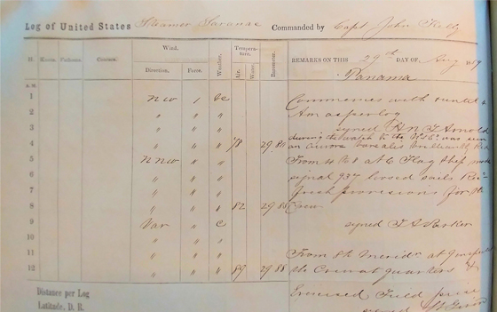
Figure 6. USS. Saranac (RG24-1) (Courtesy of the National Archives and Records Administration).
Download figure:
Standard image High-resolution image
Figure 7. USS. Sabine (RG24-2) (Courtesy of the National Archives and Records Administration).
Download figure:
Standard image High-resolution image
Figure 8. USS. St. Mary's (RG24-3) (Courtesy of the National Archives and Records Administration).
Download figure:
Standard image High-resolution image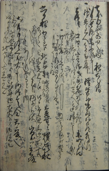
Figure 9. Reproduction of Chikusai Nikki.
Download figure:
Standard image High-resolution image
B.1. USS. Saranac (RG24-1)
- 29th day of August, 1859. Panama
- 0400
- During the watch to the N and E was seen an aurora borealis, brilliantly red.
B.2. USS. Sabine (RG24-2)
- 2nd day of September 1859. At anchor off Greytown, Friday
- At 1230 noticed the sky from about N by E to N.W. + upward to an altitude of about 35° began to assume a vermilion color, which gradually increased in intensity until about 130 when it had become of a deep rosy red & so continued until about 3, when its color had somewhat faded & finally became obscured by clouds. During the continuance of the phenomenon, heavy masses of cum. clouds were flooding over that part of the heavens which, as they passed, entirely obscured the appearance, except where they were broken or detached; and stars of the 1st, 2nd, and even of the 3rd magnitude were distinctly visible through the light.
B.3. USS. St. Mary's (RG24-3)
- 2nd day of 1859 September. At Sea
- At 12, discovered a very bright red light, bearing due north and extending over an arc of the horizon of about 70° with an altitude of about 20°.
Appendix C: Transcription and Translation of Chikusai Nikki (HJ5)
C.1. Transcription
六日夜五ツ過ゟ北ゟ少 東秋葉金比羅山之 間火光天ニ耀終夜明かた迄火光見ヘ候由 四日市桑名辺大火ニ哉と申唱候八日迄様子不訳 山田ゟハ京大坂なとニハあらすやなと申越候 右後日ニ及候へ共火事之沙汰無之全天変也 宮ゟ乗船桑名へ来候もの岐阜辺大火トノ風説也 何方も同様北方へ火光ヲ見ル
C.2. Translation
During night on 6th (1859 September 2), from around 20:00, at a little eastward from north, within the mountain of Akiba Kompira, fiery light shone in the heaven and fiery light was seen for whole night until the dawn. We discussed if Yokkaichi or Kuwana is in conflagration. However until the 8th (1859 September 4), it was not attested. From Yamada, it was rumored (conflagration broke out) in Osaka. Even later, there was no conflagration reported and everything seems a celestial omen. Those who came from Miya to Kuwana also rumored that somewhere near Gifu was in conflagration. In any places, the fiery light was seen in the northward.
Appendix D: Reproduction of Ship Log Observations during the Carrington Event
Reproduction of Chikusai Nikki (HJ5; courtesy of Izawa Library). This event seems to have attracted Chikusai's interest considerably, and its summary is found in the front cover of v.51 of Chikusai Nikki.