


Abstract
We have derived a new thermonuclear rate with an associated uncertainty for the 10B(α,p)13C reaction by evaluating the available experimental data for the first time. We provide this rate with a much smaller uncertainty than that estimated in the literature. Our rate differs significantly from the theoretical rates adopted in the current reaction rate libraries. Utilizing this new rate, we have investigated its astrophysical implications on the heavy-element (especially, p-nuclei) production in the νp-process in a stellar model of the neutrino-driven wind of type II core-collapse supernova. It shows that our rate with a much smaller uncertainty strongly constrains the nucleosynthetic results of the light p-nulcei with A ∼ 80–100. In addition, it shows that the difference between observed and predicted abundances for light p-nuclei is quite large, implying either that the present stellar model still needs modification or that additional astrophysical sources are required to account for the origin of some p-nuclei, such as 92Mo and 94Mo.
Export citation and abstract BibTeX RIS
1. Introduction
The heavy nuclei above iron observed in the solar system have been mainly produced by neutron-induced nucleosynthesis processes, such as the slow neutron-capture process (s-process; Käppeler et al. 2011) in low-mass asymptotic giant branch stars and massive red giant stars, and the rapid neutron-capture process (r-process; Arnould et al. 2007) in the supernova (SN) shock front (Käppeler et al. 1989) or the binary neutron star (BNS) mergers (Thielemann et al. 2017). On 2017 August 17 at 12:41:04 UTC, the Advanced LIGO and Advanced Virgo gravitational-wave detectors made their first observation of a BNS inspiral of GW170817 (Abbott et al. 2017). Together with the subsequent electromagnetic counterpart observations of this BNS merger, a new era of multi-messenger observations has opened, which provides us deep insight into astrophysics, dense matter, gravitation, and cosmology. The electromagnetic observation supports the long-standing suspicion that BNS mergers are the main site of r-process nucleosynthesis (e.g., see Chornock et al. 2017; Cowperthwaite et al. 2017). About half of the heavy nuclei in the solar system originate from the s-process (up to 209Bi), and the another half originate from the r-process (up to Th and U). Besides these two processes, in nature there are 35 stable nuclei on the neutron-deficient (or proton-rich) side of the valley of stability, ranging from 74Se to 196Hg, which are shielded against production by neutron-capture processes. This third class of nuclei was categorized as p-nuclei (Arnould & Goriely 2003), which amounts to less than 1% of the s- and r-element abundances, and their abundances are currently based on the analysis of meteorite data (Anders & Grevesse 1989).
Arnould (1976) and Woosley & Howard (1978) attributed the production of the p-nuclei to photodisintegration, a series of (γ, n), (γ, p), and (γ, α) reactions flowing downward through radioactive proton-rich progenitors from lead to iron, i.e., via the so-called p-process or γ-process. Such a γ-process operated on the pre-existing s-process seed in the star and was thus "secondary" in nature (or even "tertiary," since the s-process itself is secondary). It could only occur in a star that was made from the ashes of an ex-star experiencing the s-process. Arnould (1976) suggested hydrostatic oxygen burning in massive stars as the site, while Woosley & Howard (1978) discussed explosive oxygen and neon burning in an SN II as the likely site. However, the astrophysical origin of the p-nuclei is yet to be fully understood. The most successful model to date, the photo-dissociation of pre-existing neutron-rich isotopes in the oxygen-neon layer of a Type II core-collapse supernova (CCSN) or in their pre-collapse stages, can explain the lighter and heavier p-nuclei adequately; however, there still are significant discrepancies for the light p-nuclei 92,94Mo and 96,98Ru, which are largely overabundant compared to the model predictions, as well as for the Dy and Gd p-isotopes in the mass region, A = 150–160 (e.g., see Woosley & Howard 1978; Prantzos et al. 1990; Lambert 1992; Meyer 1994; Rayet et al. 1995; Rauscher et al. 2002). Such discrepancies have been reviewed in more detail by Arnould & Goriely (2003).
The discovery of a new nucleosynthesis process, the νp-process, has dramatically changed this difficult situation. The "νp-process" was first identified in Fröhlich et al. (2006a), and the term was introduced by Fröhlich et al. (2006b). It is synonymous with the "neutrino-induced rp-process" in the subsequent works (Pruet et al. 2006; Wanajo 2006). In the early neutrino-driven winds (NDWs) of a CCSN,  capture on free protons, p(
 , e+)n, gives rise to a tiny amount of free neutrons in the proton-rich matter. These neutrons immediately induce the (n,p) reactions on the β+-waiting-point nuclei, 64Ge, 68Se, and 72Kr, along the classical rp-process (Wallace & Woosley 1981; Schatz et al. 1998) path, which bypasses these waiting points quickly. Here, the νp-process starts with the seed nucleus 56Ni (not 64Ge, the first β+-waiting-point nucleus in the classical rp-process pathway), assembled from free nucleons in nuclear quasi-equilibrium (QSE) during the initial high-temperature phase (T9 > 4; where T9 is the temperature in units of 109 K). The νp-process is therefore a primary process, which does not need any pre-existing seeds. When the temperature decreases below T9 ∼ 3 (defined as the onset of a νp-process) and QSE freezes out, the νp-process starts. Unlike the r-process, the νp-process is not terminated by the exhaustion of free protons, but by the temperature decreasing below T9 = 1.5 (defined as the end of a νp-process), where proton capture slows down due to the Coulomb barrier.
All the recent hydrodynamic studies of the CCSN with neutrino transport taken into account suggest that the bulk of early SN ejecta is proton rich (e.g., Wanajo et al. 2018 and references therein). This supports the idea of the νp-process taking place in the NDWs of a CCSN. However, different works (Fröhlich et al. 2006a; Pruet et al. 2006; Wanajo 2006) end up with different outcomes. These diverse outcomes indicate that the νp-process is highly sensitive to the physical conditions of NDWs. Besides the SN conditions, there could also be uncertainties in some important nuclear reaction rates (Wanajo et al. 2011). This shows that the uncertainties in some reactions relevant to the breakout from the pp-chain region (A < 12), which affect the proton-to-seed ratio at the onset of νp-processing, might influence the nucleosynthetic outcomes. It demonstrated that 7Be(α,γ)11C and 10B(α,p)13C reactions play an important role in the temperature range's relevance to the νp-process. The impact of the 10B(α,p)13C reaction rate uncertainty on the predicted abundances is significant for p-nuclei with A ∼ 100–110. In the work of Wanajo et al. (2011), the 10B(α,p)13C reaction rate was obtained from Wagoner (1969), which was a simple theoretical estimation involving only the nonresonant (NR) reaction mechanism and no error quoted. Wanajo et al. (2011) simply assumed these rate uncertainties by arbitrary factors of 2 (or  ) and 10 (or
  ) in their sensitive studies.
In this work, we report a new thermonuclear 10B(α,p)13C reaction rate with a much smaller uncertainty in a temperature region of 1.5–5 GK, based on the solid experimental data. Using this new rate, we have investigated its astrophysical implications on the νp-process in a stellar model of the NDW of a CCSN.
2. Current Reaction Rates
Until now, the 10B(α,p)13C reaction rate adopted in the νp-process simulations and in the JINA REACLIB7 (Cyburt et al. 2010) is still the very old rate of Wagoner (1969), which is a theoretical estimation that considers only the NR reaction mechanism, but without any information on the way of calculation and the error. The NR S factor adopted by Wagoner (1969) was a constant value of SNR(E0) = 8.09 × 10⁴ MeV · b. In addition, the STARLIB8 (Sallaska et al. 2013) contains a TALYS9 calculation for this reaction rate. Here, we refer to the Wagoner (1969) rate as wag using the nomenclature in the JINA REACLIB, and the STARLIB rate as TALYS, respectively. The ratio between these two reaction rates is shown in Figure 1. The ratios between TALYS and wag are about 2.0 at 0.1 GK, and 0.1 at 10 GK, respectively. In the STARLIB database, a factor of 10 uncertainty was assumed for the calculated TALYS rate.
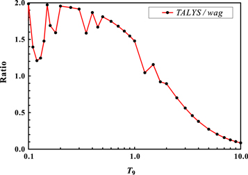
Figure 1. Ratio between TALYS rate adopted in the STARLIB and wag rate in the JINA REACLIB. Therefore, the TALYS rate has a factor of 10 uncertainty assumed in STARLIB.
Download figure:
Standard image High-resolution image3. Evaluation of Existing Data
The νp-process in the NDW of the CCSN occurs at a typical temperature region of 1.5 ∼ 3.5 GK (Wanajo et al. 2011). For the 10B(α,p)13C reaction studied, a temperature of 1.5 GK corresponds to a Gamow peak (Rolfs & Rodney 1988) at Ec.m. = 1.05 MeV with a width of Δ = 0.85 MeV, and 3.5 GK corresponds to a Gamow peak at Ec.m. = 1.85 MeV with a width of Δ = 1.72 MeV. Here, c.m. indicates the center-of-mass frame. Therefore, for the above temperature region of νp-process interest, the corresponding energy region is Ec.m. ≈ 0.7 ∼ 2.7 MeV (with a half width of Δ/2 expansion). In other words, it corresponds to an α beam energy of Eα ≈ 1.0 ∼ 3.8 MeV in the laboratory frame. In the present work, we have evaluated the cross-section data available for 10B(α,p)13C reaction in the energy region of Eα ≈ 1.0 ∼ 8.0 MeV (i.e., Ec.m. ≈ 0.7 ∼ 5.7 MeV), which are sufficient for reaction rate calculations in a temperature region of 1.5 ∼ 5 GK.
The relevant energy scheme is shown in Figure 2. As for the 10B(α,p)13C reaction, there are typically four proton groups that leave 13C in the ground state (1/2−, p0) and the excited 3.089 MeV (1/2+, p1), 3.685 MeV (3/2−, p2), and 3.854 MeV (5/2+, p3) states. All groups contribute to the total reaction cross section of 10B(α,p)13C. In fact, later the reader may find that the p2 and p3 groups (or channels) dominate the total cross section in the energy region studied, as will be discussed in detail in the following subsections.

Figure 2. Relevant energy scheme. The Gamow window is marked for a typical temperature region of 1.5 ∼ 3.5 GK, at which the 10B(α,p)13C reaction plays an important role in νp-process. As an example, four proton exit channels (p0, p1, p2, p3) are indicated for the Eα = 1.13 MeV resonance. Data are taken from Ajzenberg-Selove (1991). Here, the vertical energy scale is arbitrary (not linear).
Download figure:
Standard image High-resolution image3.1. Data in the 1.0 < Eα < 2.04 MeV Region
Shire et al. (1953) first made the relative yield measurement in this energy region and also measured the angular distributions at several energy points. Based on their nominal experimental parameters and yields listed in their Table 1, for the 1.51 MeV resonance, the differential cross sections (at θlab = 90°) are thus calculated to be 0.83, 0.23, 0.88, and 4.42 mb/sr, for p0, p1, p2, and p3 groups, respectively. The yield curves of four proton groups shown in their Figure 2 are digitized, and the data are extracted accordingly. These digitized data are then normalized to the differential cross section calculated for the 1.51 MeV resonance. Figure 3(a) shows thus obtained differential cross-section curves for each proton group at θlab = 90°. Here, the difference between c.m. and lab differential cross sections is quite small, less than 4% at maximum. According to the yield values listed in their Table 1 for the 1.64, 1.68, and 1.83 MeV resonances, the corresponding differential cross sections are calculated, and they are very consistent (with deviation less than 5%) with those shown in Figure 3(a). In addition, five separate data points, i.e., 1.13 and 1.24 MeV for p1 group (filled squares) and 1.13, 1.24, and 1.39 MeV for p2 group (filled circles), are also shown and are normalized to the 1.51 MeV resonance based on their yield values. The contributions from the p0, p1, and p2 groups relative to the p3 group are shown in Figure 3(b). It shows clearly that p3 group dominates in this energy region, except where p1 and p2 groups become important around 1.39 and 2 MeV, respectively. In fact, such p0 data derived here are consistent with the previous results (Oberg et al. 1975; Chen et al. 2003), which will be discussed in Appendix B in detail. In Section 3.4 will show that the Shire et al. (1953) data derived above match well with other experimental data within the uncertainties.
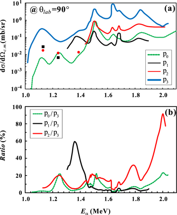
Figure 3. (a) Differential cross sections calculated for each proton group based on the yield curves shown by Shire et al. (1953), where two filled squares (for p1) and three filled circles (for p2) are calculated based on the Table 1 values of Shire et al. (1953). (b) Ratios relative to the p3 group in percentages, where the p2/p3 ratio between 1.13 ∼ 1.44 MeV is estimated based on the interpolated p2 data.
Download figure:
Standard image High-resolution image3.2. Data in the 2.10 < Eα < 8.0 MeV Region
Wilson (1975) made a complete differential cross-section and angular-distribution measurements in this energy region. The Legendre polynomial coefficients were deduced for four proton groups by fitting the angular-distribution data in terms of Legendre polynomials:
Thus, the integrated c.m. cross section for each group (pi) can be simply calculated by  . However, we found that the above coefficient
  should be divided by a factor of 2 after carefully checking his PhD thesis (Wilson 1973).10
In this work, we have calculated these integrated cross sections by a relation of
should be divided by a factor of 2 after carefully checking his PhD thesis (Wilson 1973).10
In this work, we have calculated these integrated cross sections by a relation of  . Here,
  coefficients are extracted from Figures 9–12 presented by Wilson (1975) for the energy region of 2.1 ≤ Eα ≤ 7.9 MeV; for the higher energy region of 7.9 ≤ Eα ≤ 8.0 MeV, we have reanalyzed the angular-distribution data in Wilson (1973) and obtained the Legendre polynomial coefficients,
  . The integrated cross sections are shown for each group in Figure 4(a), where the errors are calculated based on those of the
  coefficients. Figure 4(b) shows contribution of each group to the summed cross section in percentages. In general, it shows that the p2 and p3 groups make the major contribution.
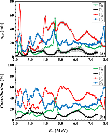
Figure 4. (a) Integrated cross section and associated statistical uncertainties for each proton group. (b) Contribution of each group to the summed cross section in percentages. The calculations are based on the data of Wilson (1973, 1975). Here, the lines connecting the data are just to guide the eyes. See the text for details.
Download figure:
Standard image High-resolution image3.3. Data in the 2.04 < Eα < 3.4 MeV Region
In this energy region, Bonner et al. (1956) measured the (α,pγ) differential cross section using an Na i γ-ray detector in the angle of θlab= 40°–50° (as shown in their Figure 3). We adopt their data up to a maximum energy of Eα = 3.4 MeV, beyond which the data are unreliable since the contaminated γ-ray that originated from 13N appeared, as explained by the authors. These (α,pγ) data actually correspond to the summed contribution of p1+p2+p3. We transferred these data to the c.m. frame and plotted them in Figure 5 (labeled as "Bonner56"). Here, we have also calculated the summed p1+p2+p3 differential cross section based on the data of Wilson (1975). The resulting "Wilson75" data are shown in Figure 5 for comparison, where an uncertainty of 15% is adopted for both data sets. In general, it shows that they are consistent within the uncertainties. Since Bonner et al. (1956) utilized a much thinner B target (7 μg cm−2) than that (∼40 μg cm−2) used by Wilson (1975), this is why the former resolved the two resonances around 2.3 MeV.

Figure 5. Comparison between data of Bonner et al. (1956) and Wilson (1975) at an angle of θlab = 45°. Bonner et al. (1956) measured the 10B(α,pγ)13C differential cross section using an Na i γ-ray detector in angle of θlab = 40°–50°, i.e., a sum of p1+p2+p3. Here, the black dots indicate the corresponding calculated sum of p1+p2+p3 based on the Wilson (1975) data.
Download figure:
Standard image High-resolution image3.4. Total Cross Section
The total cross section of the 10B(α,p)13C reaction evaluated in the energy region of Ec.m. = 0.7 ∼ 5.7 MeV is shown in Figure 6. Three experimental data sets of Shire et al. (1953), Bonner et al. (1956), and Wilson (1975), described above, are adopted in the present work. In the above Figures 3–5, the horizontal axis Eα represents the α beam energy. Here, the horizontal axis Ec.m. energy in Figure 6 is calculated by Ec.m. =  , where Δt is the energy loss of the α beam through the whole target, with the energy loss calculated by a LISE code11
(Tarasov & Bazin 2004). In addition, the Wagoner (1969) estimated cross section is shown for comparison, with a constant S factor of
, where Δt is the energy loss of the α beam through the whole target, with the energy loss calculated by a LISE code11
(Tarasov & Bazin 2004). In addition, the Wagoner (1969) estimated cross section is shown for comparison, with a constant S factor of  = 8.09 × 10⁴ MeV · b. Figure 6(b) shows clearly in an logarithm scale that the Wagoner (1969) rough estimation is quite different from the present evaluation. The Gamow windows are drawn illustratively at typical temperatures of 1.5, 3.5, and 5 GK, respectively, which are very broad for this kind of α-induced reaction.

Figure 6. Total cross section evaluated for the 10B(α,p)13C reaction (a) in a linear scale and (b) in a logarithm scale. The black dots ("Wilson75," with 15% uncertainty, gray error bars) indicate the evaluated values based on the data of Wilson (1975). The red circles ("Bonner56," with 15% uncertainty, orange error bars) indicate those evaluated values based on the data of Bonner et al. (1956). Here, the connecting lines are just to guide the eyes. The pink curve (central value) and the associated blue error band (50% uncertainty estimated) indicate the presently evaluated "Shire53" data based on the extracted ones from Shire et al. (1953). For comparison, the Wagoner (1969) estimation is shown with a green solid line. In addition, the Gamow windows are illustratively shown for typical temperatures of 1.5, 3.5, and 5 GK, respectively. See the text for details.
Download figure:
Standard image High-resolution imageAs for the Wilson (1975) data in the region of Ec.m. = 1.52 ∼ 5.67 MeV, the total cross section is calculated by summing the four contributions (p0+p1+p2+p3) shown in Figure 4(a), with a conservatively estimated uncertainty of 15% (systematical: ∼7%, averaged statistical: ∼3%, target thickness effect: ∼10%). As for the Bonner et al. (1956) data in the region of Ec.m. = 1.46 ∼ 2.42 MeV, the total cross section has been calculated by adding the p0 contribution, about 8% ∼ 20%, based on the proton branching ratios, as shown in Figures 3(b) and 4(b). These (α,pγ) data were measured in the angle of θlab = 40°–50° (i.e., θlab ≈ 45°), and hence the total cross section can be obtained reasonably using an isotropic angular distribution. Here, we estimate a conservative uncertainty of 15% for the evaluated Bonner et al. (1956) data, i.e., 10% for the systematical one in the original (α,pγ) data, 10% for the angular-distribution effect, and 5% for the p0 correction. In general, the Wilson (1975) and Bonner et al. (1956) data agree well close to the overlapped energy region, as shown in Figure 6.
As for the Shire et al. (1953) data in the region of Ec.m. = 0.7 ∼ 1.45 MeV, we have summed those four contributions, as shown in Figure 3(a), by assuming an isotropic angular distribution. Here, an angular-distribution factor, f, is defined via the relation between the total cross section and the differential cross section at θlab = 90°, as σtot = f × 4π  (where f is unity for an isotropic angular distribution). The f values can be calculated based on the angular-distribution parameters listed in their Table 2. For the dominant p3 group, the f factors are calculated to be 1.24, 1.18, 0.78, 1.06, and 0.95 for the 1.13, 1.51, 1.64, 1.68, and 1.83 MeV resonances, respectively. Therefore, the isotropic distribution assumed in this work may deviate from reality by no more than 24% on resonances. As stated by Shire et al. (1953, p. 1209), "Owing to the difficulty of estimating the thicknesses of the targets used, and their gradual deterioration under bombardment our results, which are given in Table 4, are subject to considerable error, but are, we believe correct to about a factor of two," we conservatively estimate the presently derived Shire et al. (1953) data with a relative large uncertainty of 50%, which is further constrained by the Bonner et al. (1956) data.
In addition, close to the lowest Eα = 1.13 MeV resonance (Ec.m. ≈ 0.8 MeV as shown in Figure 6), Ajzenberg-Selove (1986) compiled a resonance at Eα = 0.82 MeV (i.e., Ex(14N) = 12.20 MeV, Ec.m. = 0.59 MeV), while Ajzenberg-Selove (1991) slightly modified this resonance to Eα = 0.95 MeV (i.e., Ex(14N) = 12.29 MeV, Ec.m. = 0.68 MeV). Since there is no clear α contribution observed for this state so far (Shire et al. 1953; Ajzenberg-Selove 1986, 1991), here we neglected the contribution from this resonance in the present reaction rate calculation. Although a nonvanishing Gamow tail at energies below Ec.m. = 0.7 MeV for 1.5 GK is shown in Figure 6(b), its contribution to the reaction rate can be neglected for temperatures below 1.5 GK. For instance, adding a linear or constant extrapolation for the low-energy region of Ec.m. < 0.7 MeV does not affect the rate above 1.5 GK significantly, only about 3%, which is much smaller than the corresponding rate uncertainties of ∼50%.
4. New Reaction Rate
The thermonuclear 10B(α,p)13C rate as a function of temperature has been calculated by numerical integration of our evaluated experimental cross-section data (all those shown in Figure 6) by Rolfs & Rodney (1988):

In addition, the effect of thermally excited states of the target nucleus (10B) is considered in the total reaction rate at high temperatures (Rolfs & Rodney 1988). The first and second excited states are in 10B located at Ex = 0.718 (1+), 1.740 (0+) MeV, respectively. In fact, the probability of populating the first excited state of the target nucleus, 10B, is only about 7% at 5 GK and 16% at 10 GK, respectively; while the probability of populating the second excited state of 10B is only about 2% even at 10 GK. Therefore, these thermal effects can actually be neglected below 5 GK. The present 10B(α,p)13C reaction rate and the associated uncertainties (lower and upper limits) are summarized in Table 1. The Present mean rate can be parameterized by the standard format of Rauscher & Thielemann (2000),
with a fitting error of less than 0.3% over the temperature region of 1.5–5 GK.
Table 1. Thermonuclear Rates of 10B(α,p)13C (in Units of cm3 s−1 mol−1)
| Present Work | TALYS | wag | |||
|---|---|---|---|---|---|
| T9 | Mean | Lower | Upper | ||
| 1.5 | 3.19 × 10+04 | 1.65 × 10+04 | 4.76 × 10+04 | 2.04 × 10+04 | 1.76 × 10+04 |
| 1.6 | 4.92 × 10+04 | 2.57 × 10+04 | 7.32 × 10+04 | 2.45 × 10+04 | 2.84 × 10+04 |
| 1.7 | 7.24 × 10+04 | 3.82 × 10+04 | 1.07 × 10+05 | 4.03 × 10+04 | 4.40 × 10+04 |
| 1.8 | 1.02 × 10+05 | 5.45 × 10+04 | 1.51 × 10+05 | 6.16 × 10+04 | 6.59 × 10+04 |
| 1.9 | 1.40 × 10+05 | 7.52 × 10+04 | 2.05 × 10+05 | 8.87 × 10+04 | 9.59 × 10+04 |
| 2.0 | 1.85 × 10+05 | 1.01 × 10+05 | 2.70 × 10+05 | 1.22 × 10+05 | 1.36 × 10+05 |
| 2.1 | 2.39 × 10+05 | 1.32 × 10+05 | 3.47 × 10+05 | 1.63 × 10+05 | 1.88 × 10+05 |
| 2.2 | 3.01 × 10+05 | 1.68 × 10+05 | 4.36 × 10+05 | 2.12 × 10+05 | 2.56 × 10+05 |
| 2.3 | 3.73 × 10+05 | 2.10 × 10+05 | 5.37 × 10+05 | 2.69 × 10+05 | 3.41 × 10+05 |
| 2.4 | 4.54 × 10+05 | 2.59 × 10+05 | 6.50 × 10+05 | 3.35 × 10+05 | 4.46 × 10+05 |
| 2.5 | 5.44 × 10+05 | 3.14 × 10+05 | 7.75 × 10+05 | 4.04 × 10+05 | 5.76 × 10+05 |
| 2.6 | 6.43 × 10+05 | 3.75 × 10+05 | 9.13 × 10+05 | 4.98 × 10+05 | 7.34 × 10+05 |
| 2.7 | 7.51 × 10+05 | 4.43 × 10+05 | 1.06 × 10+06 | 5.97 × 10+05 | 9.23 × 10+05 |
| 2.8 | 8.69 × 10+05 | 5.17 × 10+05 | 1.22 × 10+06 | 7.08 × 10+05 | 1.15 × 10+06 |
| 2.9 | 9.94 × 10+05 | 5.98 × 10+05 | 1.39 × 10+06 | 8.32 × 10+05 | 1.41 × 10+06 |
| 3.0 | 1.13 × 10+06 | 6.86 × 10+05 | 1.57 × 10+06 | 9.66 × 10+05 | 1.72 × 10+06 |
| 3.1 | 1.27 × 10+06 | 7.80 × 10+05 | 1.77 × 10+06 | 1.12 × 10+06 | 2.08 × 10+06 |
| 3.2 | 1.42 × 10+06 | 8.81 × 10+05 | 1.97 × 10+06 | 1.29 × 10+06 | 2.49 × 10+06 |
| 3.3 | 1.58 × 10+06 | 9.88 × 10+05 | 2.18 × 10+06 | 1.47 × 10+06 | 2.96 × 10+06 |
| 3.4 | 1.75 × 10+06 | 1.10 × 10+06 | 2.39 × 10+06 | 1.67 × 10+06 | 3.50 × 10+06 |
| 3.5 | 1.92 × 10+06 | 1.22 × 10+06 | 2.62 × 10+06 | 1.88 × 10+06 | 4.10 × 10+06 |
| 4.0 | 2.88 × 10+06 | 1.90 × 10+06 | 3.86 × 10+06 | 3.21 × 10+06 | 8.38 × 10+06 |
| 4.5 | 3.98 × 10+06 | 2.72 × 10+06 | 5.25 × 10+06 | 4.94 × 10+06 | 1.53 × 10+07 |
| 5.0 | 5.19 × 10+06 | 3.64 × 10+06 | 6.74 × 10+06 | 6.97 × 10+06 | 2.56 × 10+07 |
Note. Here, the mean, lower, and upper rates are calculated numerically by Equation (2) for a certain temperature when cross sections (see Figure 6) are set, point-by-point, to its mean (or Centroid) value, lower, and upper bounds, respectively.
Download table as: ASCIITypeset image
Figure 7 shows the comparison between our rate and TALYS and wag rates. It shows that our new rate deviates significantly from two theoretical rates in the whole temperature region (see the small inserted figure shown in Figure 7). Although the TALYS rate agree with the present one within the uncertainties, our rate is constrained by a much smaller uncertainty. In the temperature region of 1.5–3.5 GK of astrophysical νp-process interest, our rate deviates from the old wag rate by about factors of 0.5 ∼ 1.8, although the corresponding cross-section data are quite different (see Figure 6). This is mainly because of the very broad Gamow window for this kind of (α,p) reaction. It should be noted that our rate is, for the first time, constrained in a much smaller uncertainty, about (37 ∼ 50)% in 1.5–5 GK, based on the solid experimental data. The remaining uncertainty mainly originates from the 50% uncertainty estimated for the Shire et al. (1953) data in the energy region of Eα = 1–2 MeV, where a precise cross-section measurement is strongly desired to reduce further the uncertainty.

Figure 7. Thermonuclear 10B(α,p)13C reaction rates (in units of cm3 s−1 mol−1). The ratios between the Present and TALYS and wag rates are shown in the inserted panel.
Download figure:
Standard image High-resolution image5. Astrophysical Implications
In order to examine impact of the new thermonuclear 10B(α,p)13C rate on the νp-process, we used a semi-analytic NDW model and the reaction network code to obtain the thermodynamic trajectories of neutrino-driven outflows and productions of the νp-process. The parameters of the wind model are the "standard" ones (the neutron star mass of 1.4 M⊙, the neutrino luminosity of 1052 erg s−1, the wind-termination radius of 300 km, and the initial electron fraction of 0.6 decreasing to 0.55 at 3 GK), which represent typical SN conditions. More details for the model, as well as the reaction network code, can be found in Wanajo et al. (2011).
The stellar nucleosynthetic results are summarized in Figure 8. Here, three different thermonuclear 10B(α,p)13C rates, i.e., the Present, TALYS, and wag rates, are implemented in the network calculations. It shows that the mass fractions predicted with three different rates are very consistent for a mass region of A < 90, although there is a small deviation at A ∼ 75 as shown in Figure 8(b); while for the A > 90 mass region, comparing to wag rate, ours predicts a larger abundance up to a factor of ∼3 for A ∼ 130. The TALYS rate more evidently shows this impact. This is a consequence of the fact that the Present and TALYS rates are smaller than the wag rate at ∼3 GK, which is the temperature approximately the end of the heavy seed production. This 10B(α,p)13C rate also competes with the triple-α process at this temperature (Figure 10 in Wanajo et al. 2011). The resulting higher proton-to-seed ratio leads to a greater amount of the heavy isotope. In addition, the impact of the Present rate uncertainties (the lower and upper limits listed in Table 1) and that of the TALYS rate uncertainties (a factor of 10) are shown in Figure 8(b), respectively. Even with the Present smaller uncertainties (about 37% ∼ 50%) in the temperature region of 1.5–3.5 GK of νp-process interest, their impact is still significant on the heavy-element (A > 110) production. Although the TALYS results (with the mean value) are consistent with ours within the present uncertainties, a factor of 10 uncertainty assumed for this theoretical rate results in huge uncertainties on the heavy-element (A > 110) production as shown. Therefore, our smaller rate of uncertainty constrains the nucleosynthetic results or more strongly constrains even the stellar model. Similar to Figure 14(c) plotted in Wanajo et al. (2011), the corresponding result is shown in Figure 8(c) for some p-nuclei. For clarity, the digital numbers for the predicted abundances are listed in Table 2.
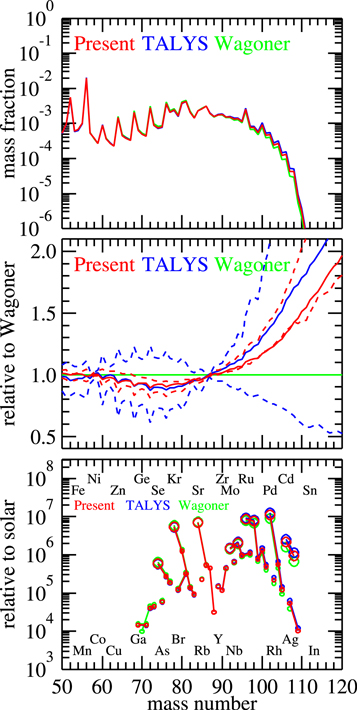
Figure 8. Comparison of the nucleosynthetic results for different 10B(α,p)13C reaction rates as a function of the atomic mass number. The color coding corresponds to different rates: red for the present rate, blue for the TALYS rate, and green for the wag rate, respectively. (a) The mass fractions (with values greater than 10−6); (b) their ratios relative to those for the wag rate, where the impacts of uncertainties in the Present and TALYS rates are shown accordingly; (c) nucleosynthetic p-abundances relative to their solar values, i.e., production factors (where those lower than 104 are omitted). In the bottom panel, the names of elements (connected by a line for a given element) are specified in the upper (even Z) and lower (odd Z) sides at their lightest mass numbers. Please refer to the similar caption of Wanajo et al. (2011).
Download figure:
Standard image High-resolution imageTable 2. Production Factors Predicted for Different Reaction Rates of 10B(α,p)13C, Relative to the Solar Abundances
| Present Rate | TALYS Rate | wag Rate | |||||||
|---|---|---|---|---|---|---|---|---|---|
| Z | A | p-nuclei | Mean | Lower | Upper | Mean | Lower | Upper | |
| 34 | 74 | 77Se | 5.90E+05 | 5.52E+05 | 6.09E+05 | 5.77E+05 | 4.70E+05 | 7.26E+05 | 6.42E+05 |
| 34 | 76 | 2.71E+05 | 2.47E+05 | 2.85E+05 | 2.63E+05 | 1.94E+05 | 3.58E+05 | 3.00E+05 | |
| 34 | 77 | 1.86E+05 | 1.74E+05 | 1.91E+05 | 1.81E+05 | 1.46E+05 | 2.30E+05 | 2.03E+05 | |
| 34 | 78 | 1.44E+02 | 1.50E+02 | 1.28E+02 | 1.38E+02 | 1.87E+02 | 1.26E+02 | 1.49E+02 | |
| 34 | 80 | 6.71E-02 | 7.35E-02 | 5.69E-02 | 6.45E-02 | 1.06E-01 | 5.11E-02 | 6.77E-02 | |
| 35 | 79 | 1.22E+05 | 1.15E+05 | 1.24E+05 | 1.19E+05 | 9.99E+04 | 1.45E+05 | 1.32E+05 | |
| 35 | 81 | 3.19E+05 | 3.04E+05 | 3.28E+05 | 3.15E+05 | 2.65E+05 | 3.74E+05 | 3.42E+05 | |
| 36 | 78 | 78Kr | 5.39E+06 | 5.04E+06 | 5.52E+06 | 5.24E+06 | 4.26E+06 | 6.57E+06 | 5.85E+06 |
| 36 | 80 | 1.26E+06 | 1.18E+06 | 1.31E+06 | 1.24E+06 | 9.85E+05 | 1.55E+06 | 1.37E+06 | |
| 36 | 82 | 1.37E+05 | 1.34E+05 | 1.37E+05 | 1.35E+05 | 1.25E+05 | 1.49E+05 | 1.43E+05 | |
| 36 | 83 | 9.16E+04 | 9.02E+04 | 9.10E+04 | 9.06E+04 | 8.64E+04 | 9.64E+04 | 9.51E+04 | |
| 36 | 84 | 7.43E+00 | 8.37E+00 | 6.28E+00 | 7.29E+00 | 1.26E+01 | 5.20E+00 | 7.19E+00 | |
| 37 | 85 | 2.25E+05 | 2.20E+05 | 2.28E+05 | 2.25E+05 | 2.04E+05 | 2.42E+05 | 2.33E+05 | |
| 37 | 87 | 1.14E-03 | 1.41E-03 | 8.83E-04 | 1.13E-03 | 2.83E-03 | 6.14E-04 | 1.05E-03 | |
| 38 | 84 | 84Sr | 6.99E+06 | 6.82E+06 | 7.08E+06 | 6.96E+06 | 6.29E+06 | 7.66E+06 | 7.31E+06 |
| 38 | 86 | 5.31E+05 | 5.28E+05 | 5.36E+05 | 5.36E+05 | 5.06E+05 | 5.50E+05 | 5.44E+05 | |
| 38 | 87 | 4.40E+05 | 4.45E+05 | 4.39E+05 | 4.46E+05 | 4.45E+05 | 4.33E+05 | 4.44E+05 | |
| 38 | 88 | 3.13E+04 | 3.21E+04 | 3.09E+04 | 3.18E+04 | 3.31E+04 | 2.95E+04 | 3.11E+04 | |
| 39 | 89 | 1.47E+05 | 1.51E+05 | 1.46E+05 | 1.50E+05 | 1.58E+05 | 1.38E+05 | 1.46E+05 | |
| 40 | 90 | 1.17E+05 | 1.21E+05 | 1.17E+05 | 1.21E+05 | 1.27E+05 | 1.09E+05 | 1.16E+05 | |
| 40 | 91 | 4.42E+05 | 4.61E+05 | 4.37E+05 | 4.55E+05 | 4.97E+05 | 3.97E+05 | 4.30E+05 | |
| 40 | 92 | 1.20E+03 | 1.37E+03 | 1.07E+03 | 1.23E+03 | 1.98E+03 | 8.15E+02 | 1.11E+03 | |
| 41 | 93 | 6.47E+05 | 6.86E+05 | 6.38E+05 | 6.72E+05 | 7.64E+05 | 5.53E+05 | 6.16E+05 | |
| 42 | 92 | 92Mo | 1.47E+06 | 1.55E+06 | 1.45E+06 | 1.52E+06 | 1.71E+06 | 1.27E+06 | 1.41E+06 |
| 42 | 94 | 94Mo | 2.06E+06 | 2.22E+06 | 2.02E+06 | 2.16E+06 | 2.58E+06 | 1.70E+06 | 1.94E+06 |
| 42 | 95 | 9.65E+05 | 1.04E+06 | 9.60E+05 | 1.02E+06 | 1.17E+06 | 8.06E+05 | 9.05E+05 | |
| 42 | 96 | 4.02E+03 | 4.74E+03 | 3.57E+03 | 4.21E+03 | 7.34E+03 | 2.48E+03 | 3.54E+03 | |
| 42 | 97 | 1.10E+06 | 1.23E+06 | 1.06E+06 | 1.17E+06 | 1.57E+06 | 7.96E+05 | 9.77E+05 | |
| 42 | 98 | 2.43E-03 | 3.21E-03 | 1.90E-03 | 2.53E-03 | 7.17E-03 | 1.06E-03 | 2.00E-03 | |
| 44 | 96 | 96Ru | 8.54E+06 | 9.42E+06 | 8.41E+06 | 9.12E+06 | 1.15E+07 | 6.55E+06 | 7.74E+06 |
| 44 | 98 | 98Ru | 7.57E+06 | 8.52E+06 | 7.48E+06 | 8.23E+06 | 1.09E+07 | 5.53E+06 | 6.70E+06 |
| 44 | 99 | 7.67E+05 | 8.63E+05 | 7.70E+05 | 8.43E+05 | 1.09E+06 | 5.66E+05 | 6.76E+05 | |
| 44 | 100 | 1.34E+06 | 1.54E+06 | 1.34E+06 | 1.50E+06 | 2.08E+06 | 9.21E+05 | 1.14E+06 | |
| 44 | 101 | 4.83E+05 | 5.65E+05 | 4.84E+05 | 5.45E+05 | 7.84E+05 | 3.20E+05 | 4.07E+05 | |
| 44 | 102 | 3.26E+02 | 4.20E+02 | 2.81E+02 | 3.56E+02 | 8.20E+02 | 1.54E+02 | 2.59E+02 | |
| 44 | 104 | 3.34E-02 | 4.59E-02 | 2.69E-02 | 3.65E-02 | 1.10E-01 | 1.30E-02 | 2.54E-02 | |
| 45 | 103 | 2.19E+05 | 2.61E+05 | 2.21E+05 | 2.51E+05 | 3.79E+05 | 1.36E+05 | 1.78E+05 | |
| 46 | 102 | 102Pd | 1.10E+07 | 1.31E+07 | 1.10E+07 | 1.25E+07 | 1.88E+07 | 6.96E+06 | 9.05E+06 |
| 46 | 104 | 5.62E+05 | 6.87E+05 | 5.70E+05 | 6.59E+05 | 1.06E+06 | 3.30E+05 | 4.44E+05 | |
| 46 | 105 | 1.23E+05 | 1.51E+05 | 1.24E+05 | 1.44E+05 | 2.38E+05 | 7.00E+04 | 9.52E+04 | |
| 46 | 106 | 4.65E+01 | 6.34E+01 | 4.01E+01 | 5.28E+01 | 1.43E+02 | 1.85E+01 | 3.40E+01 | |
| 46 | 108 | 1.86E+00 | 2.61E+00 | 1.56E+00 | 2.12E+00 | 6.45E+00 | 6.66E-01 | 1.31E+00 | |
| 46 | 110 | 1.23E-02 | 1.84E-02 | 9.73E-03 | 1.40E-02 | 5.48E-02 | 3.64E-03 | 8.30E-03 | |
| 47 | 107 | 5.36E+04 | 6.82E+04 | 5.40E+04 | 6.40E+04 | 1.18E+05 | 2.70E+04 | 3.91E+04 | |
| 47 | 109 | 1.01E+04 | 1.34E+04 | 9.82E+03 | 1.20E+04 | 2.61E+04 | 4.37E+03 | 6.95E+03 | |
| 48 | 106 | 106Cd | 2.13E+06 | 2.67E+06 | 2.16E+06 | 2.54E+06 | 4.45E+06 | 1.13E+06 | 1.59E+06 |
| 48 | 108 | 108Cd | 9.40E+05 | 1.22E+06 | 9.40E+05 | 1.13E+06 | 2.21E+06 | 4.41E+05 | 6.59E+05 |
| 48 | 110 | 4.97E+03 | 6.68E+03 | 4.75E+03 | 5.89E+03 | 1.38E+04 | 1.99E+03 | 3.29E+03 | |
| 48 | 111 | 9.32E+02 | 1.27E+03 | 8.69E+02 | 1.10E+03 | 2.80E+03 | 3.47E+02 | 6.03E+02 | |
| 48 | 112 | 7.68E+00 | 1.11E+01 | 6.54E+00 | 8.91E+00 | 2.98E+01 | 2.36E+00 | 4.86E+00 | |
| 48 | 113 | 4.45E-03 | 7.04E-03 | 3.36E-03 | 5.07E-03 | 2.54E-02 | 1.05E-03 | 2.74E-03 | |
| 48 | 114 | 7.32E-04 | 1.13E-03 | 5.80E-04 | 8.41E-04 | 3.68E-03 | 1.82E-04 | 4.39E-04 | |
| 49 | 113 | 1.26E+03 | 1.71E+03 | 1.20E+03 | 1.48E+03 | 3.75E+03 | 4.49E+02 | 7.67E+02 | |
| 49 | 115 | 3.58E-02 | 5.63E-02 | 2.77E-02 | 4.10E-02 | 1.97E-01 | 8.20E-03 | 2.09E-02 | |
| 50 | 112 | 112Sn | 1.82E+03 | 2.48E+03 | 1.71E+03 | 2.14E+03 | 5.46E+03 | 6.54E+02 | 1.13E+03 |
| 50 | 114 | 114Sn | 2.41E+02 | 3.25E+02 | 2.35E+02 | 2.84E+02 | 6.87E+02 | 8.66E+01 | 1.44E+02 |
| 50 | 115 | 115Sn | 2.39E+02 | 3.26E+02 | 2.28E+02 | 2.80E+02 | 7.22E+02 | 7.97E+01 | 1.39E+02 |
| 50 | 116 | 2.33E+00 | 3.24E+00 | 2.18E+00 | 2.72E+00 | 7.68E+00 | 7.17E-01 | 1.31E+00 | |
| 50 | 117 | 1.16E+00 | 1.63E+00 | 1.06E+00 | 1.34E+00 | 4.10E+00 | 3.35E-01 | 6.33E-01 | |
| 50 | 118 | 1.58E-01 | 2.22E-01 | 1.46E-01 | 1.82E-01 | 5.49E-01 | 4.48E-02 | 8.39E-02 | |
| 50 | 119 | 1.75E-01 | 2.45E-01 | 1.63E-01 | 2.02E-01 | 5.97E-01 | 4.96E-02 | 9.16E-02 | |
| 50 | 120 | 2.28E-04 | 3.57E-04 | 1.80E-04 | 2.57E-04 | 1.28E-03 | 4.41E-05 | 1.13E-04 | |
| 51 | 121 | 5.28E-02 | 7.55E-02 | 4.77E-02 | 6.00E-02 | 1.97E-01 | 1.32E-02 | 2.61E-02 | |
| 52 | 120 | 120Te | 6.07E+00 | 8.57E+00 | 5.59E+00 | 6.96E+00 | 2.14E+01 | 1.63E+00 | 3.09E+00 |
| 52 | 122 | 2.72E-02 | 3.92E-02 | 2.42E-02 | 3.05E-02 | 1.06E-01 | 6.40E-03 | 1.30E-02 | |
| 52 | 123 | 2.52E-02 | 3.68E-02 | 2.22E-02 | 2.81E-02 | 1.04E-01 | 5.61E-03 | 1.17E-02 | |
| 52 | 124 | 4.77E-04 | 7.35E-04 | 3.86E-04 | 5.27E-04 | 2.48E-03 | 8.79E-05 | 2.16E-04 | |
| 52 | 125 | 3.35E-04 | 4.92E-04 | 2.92E-04 | 3.66E-04 | 1.47E-03 | 6.85E-05 | 1.47E-04 | |
| 52 | 126 | 2.68E-06 | 4.32E-06 | 2.03E-06 | 2.89E-06 | 1.71E-05 | 4.08E-07 | 1.15E-06 | |
| 53 | 127 | 1.10E-05 | 1.60E-05 | 9.62E-06 | 1.18E-05 | 4.88E-05 | 2.11E-06 | 4.52E-06 | |
| 54 | 124 | 124Xe | 4.22E-02 | 6.03E-02 | 3.80E-02 | 4.64E-02 | 1.62E-01 | 9.47E-03 | 1.90E-02 |
| 54 | 126 | 126Xe | 5.98E-03 | 8.61E-03 | 5.32E-03 | 6.48E-03 | 2.49E-02 | 1.22E-03 | 2.53E-03 |
| 56 | 130 | 130Ba | 1.01E-04 | 1.41E-04 | 9.54E-05 | 1.10E-04 | 4.09E-04 | 2.01E-05 | 3.81E-05 |
| 56 | 132 | 132Ba | 1.82E-05 | 2.60E-05 | 1.71E-05 | 2.00E-05 | 8.11E-05 | 3.34E-06 | 6.54E-06 |
Note. Here, those production factors less than the order of 10−6 are omitted where p-nuclei are indicated in the third column.
Because 94Mo was suggested to be most likely produced primarily by the νp-process (Fröhlich et al. 2006b), we have normalized both the predicted and observed solar abundances of 94Mo as the reference of unity shown in Figure 9, where those for other p-nuclei are relative to 94Mo. Here, the error bars of the observed solar abundances (Anders & Grevesse 1989) are apparent for 74Se, 78Kr, and 92Mo, while others are smaller than the point size. The predicted abundances shown in Figure 9 are normalized based on the values listed in Table 2. The impact of our new rate on the p-nuclei production can be clearly seen in 78Kr, 84Sr, 96,98Ru, 102Pd, and 106,108Cd. Although the differences cannot be regarded as very large compared to that of wag, our better uncertainty estimation can provide much stronger constraint. Furthermore, it shows that the trends between the observed and predicted abundances are quite different, although different model parameters, e.g., the electron fraction, can affect the production ratios. Namely, our new result implies that a smaller electron fraction will be relevant for consistent relative abundances of p-isotopes over the mass range of A ∼ 80–100. Nevertheless, the underabundances of 92Mo and 94Mo relative to the neighboring p-isotopes cannot be cured. For these reasons, our result might imply that: (1) the present νp-process stellar model (itself or model parameters) still needs some modifications, and (2) the NDW of the CCSN is not the major origin of some light p-nuclei, such as 92Mo and 94Mo.

Figure 9. Relative abundances of p-nuclei in the mass region of A = 74 ∼ 108. Here, observed and all predicted abundances of 94Mo are normalized as unity, and those for the remaining nuclei are drawn relative to this reference. The impacts of uncertainties in the Present and TALYS rates are shown accordingly. See the text for more details.
Download figure:
Standard image High-resolution image6. Summary and Conclusion
We have derived a new thermonuclear rate of the 10B(α,p)13C reaction based on the evaluated experimental data in the temperature region of 1.5–5 GK. Our new rate differs significantly from the previous theoretical rates, which are adopted in the current reaction rate libraries. The astrophysical impact of our new 10B(α,p)13C rate on the heavy-element production in the νp-process has been investigated under a stellar model of the NDW of a type II core-collapse SN. It shows that the mass fraction predicted with the Present and wag rates is very consistent for mass region of A < 90, while our rate predicts larger abundances for A > 90 mass region, up to a factor of ∼3 for A ∼ 130. With the present smaller uncertainties, their impact on the heavy-element (A > 110) production is still significant. However, for the first time, we provide this rate in the νp-process temperatures (1.5–3.5 GK) with a much smaller uncertainty of (37 ∼ 50)%, with which we can strongly constrain the nucleosynthetic results. Furthermore, it shows that the predicted p-nuclei abundances are quite different from those observed ones, which might imply that the present νp-process stellar model (itself or parameters) still needs some modifications, or that the NDW of the CCSN is not the major origin of some light p-nuclei (such as 92Mo and 94Mo). Furthermore, it is worth noting that the uncertainties in this 10B(α,p)13C rate are still large, and hence a precise cross-section measurement for this reaction is desired in the energy region below Eα = 2 MeV.
This work was financially supported by the National Key Research and Development Program of China (2016YFA0400503), the National Natural Science Foundation of China (No. 11675229, 11490562, 11825504). S.W. gratefully acknowledges financial support from the RIKEN iTHES Project, the JSPS Grants-in-Aid for Scientific Research (26400232, 26400237), and JSPS and CNRS under the Japan–France Research Cooperative Program.
Appendix:
Based on the discussions made in Sections 3.1 and 3.2, we know that the p0 group, in general, plays only a minor role in calculating the total cross section of 10B(α,p)13C. However, in order to check consistency of the previous results, the differential cross sections available for this p0 group are compared at θc.m. ≈ 50° and θlab = 90°, 135°, and will be discussed below.
Appendix A: Data at θc.m. ≈ 50°
The deduced differential cross sections at θc.m. ≈ 50° are shown in Figure 10. The time-reversal reaction, 13C(p,α)10B, was previously studied by Oberg et al. (1975), where the differential cross-section and angular-distribution measurements were carried out for the (p,α0) channel. Here, we extracted their differential cross section measured at θlab = 40°, as shown in their Figure 4. This laboratory angle corresponds to a c.m. angle range of 47 4 ∼ 525, i.e., an average value of θc.m. ≈ 50°. The extracted differential cross section was then transferred to the c.m. frame and ultimately converted to those of the forward reaction of 10B(α,p0)13C (labeled "Oberg75 (Reverse)") by the well-known detailed balance principle (Blatt & Weisskopf 2010). An uncertainty of 10% is estimated for the "Oberg75 (Reverse)" data sets. Spasskiǐ et al. (1966) measured the excitation function and angular distribution for (α,p0) channel in the region of 9.1 ≤ Eα ≤ 26.1 MeV. We extracted the differential cross-section data at θc.m. ≈ 50° from their Figure 2 and converted to the c.m. frame (labeled "Spasskii66"). An uncertainty of 20% is estimated for the "Spasskii66" data sets. The differential cross-section data at θc.m. = 50° have been calculated based on the Legendre polynomial coefficients shown in Figure 9 of Wilson (1975) for the energy region of 2.10 ≤ Eα ≤ 7.90 MeV, with an estimated uncertainty of 15%; for the higher energy region of 7.95 ≤ Eα ≤ 10.75 MeV, we have reanalyzed the angular-distribution data in Wilson (1973) and obtained the Legendre polynomial coefficients. Here, we estimate a relatively larger uncertainty of 20% for these higher energy data. It shows that all existing data in the wide energy region are very consistent within the uncertainties.

Figure 10. Differential cross section for the p0 group at θc.m. ≈ 50°. The black dots: "Wilson75," red circles: "Oberg75 (Reverse)," and green dots: "Spasskii66," indicate the calculated values based on the data of Wilson (1973, 1975), Oberg et al. (1975), and Spasskiǐ et al. (1966), respectively.
Download figure:
Standard image High-resolution imageAppendix B: Data at θlab = 90°
The deduced differential cross sections of the (α,p0) channel at θlab = 90° are compared in Figure 11. The method for calculating the "Wilson75" and "Oberg75 (Reverse)" data was discussed in the previous Appendix A. Chen et al. (2003) provided the differential cross-section data (see their Table 1) in the energy range of 1.4 ∼ 3.3 MeV. Owing to a very thin natural B target (∼3.5 μg cm−2), two fine structures around Eα = 2.3 MeV (i.e., resonances at 2.174 and 2.281 MeV of Ajzenberg-Selove 1991) and Eα = 1.65 MeV (i.e., resonances at 1.645 and 1.68 MeV of Ajzenberg-Selove 1991), were clearly resolved. Wilson (1975) only observed a broad peak around 2.3 MeV using a much thicker B target (∼40 μg cm−2). Here, the data of Chen et al. (2003) are multiplied by a factor of 1.7 to achieve a better consistency between these three data sets. An uncertainty of 10% is indicated for the "Chen03" data. Derivation of the "Shire53" data has been already described in Section 3.1 in detail, and here, an uncertainty of 50% was estimated for these data.

Figure 11. Differential cross section for the p0 group at θlab = 90°. The pink curve (central value) and the associated blue error band (50% of the uncertainty estimated) indicate the calculated results based on the yield curve of Shire et al. (1953). The black dots: "Wilson75," red dots: "Chen03 (×1.7)," and green circles: "Oberg75 (Reverse)" indicate the calculated values based on the data of Wilson (1975), Chen et al. (2003), and Oberg et al. (1975), respectively. Lines connecting the data points are just to guide the eyes.
Download figure:
Standard image High-resolution imageAppendix C: Data at θlab = 135°
Figure 12 shows the lab differential cross sections of the (α,p0) channel at θlab = 135°, where the experimental values of Giorginis et al. (1996) are compared with the calculated values based on the Bi parameters of Wilson (1975). Although the amplitudes of same resonant peak are different because different target thicknesses were utilized in two experiments, both data are very consistent in the NR energy region above Eα = 4.85 MeV. In addition, those data Chen et al. (2003) measured at θlab = 90°, multiplying by a factor of 1.7 adopted above, are compared in the figure, and they are consistent with other two data in the NR region (where the angular-distribution effect is close to isotropic, i.e., f ≈ 1.0; He et al. 2018). It demonstrates again that the data of Chen et al. (2003) should be corrected by a factor of ∼1.7. We think that the classical Rutherford backscattering cross section at 1.8 MeV on the light nuclide 10B (at 90°) utilized to calibrate those of 10B(α,p)13C by Chen et al. (2003) is not reliable compared to the traditional method utilized by Giorginis et al. (1996), i.e., the Rutherford backscattering on heavy Ta backing at 135°.

Figure 12. Laboratory differential cross sections for the p0 group. At a scattering angle of θlab = 135°, the "Wilson75" and "Giorginis96" data are compared. The filled squares represent the calculated values based on the Bi coefficients of Wilson (1975), and the hollow circles represent the experimental values of Giorginis et al. (1996). In addition, the experimental data of Chen et al. (2003) measured at θlab = 90°, multiplied by a factor of 1.7, are shown as the red dots for comparison. Lines connecting the data points are just to guide the eyes.
Download figure:
Standard image High-resolution image
Footnotes
- 7
JINA REACLIB Database, https://jinaweb.org/reaclib/db/.
- 8
- 9
TALYS, http://www.talys.eu/home/.
- 10
- 11
LISE, http://lise.nscl.msu.edu/.