


Abstract
The X-ray afterglow plateau emission observed in many gamma-ray bursts (GRBs) has been interpreted as being fueled either by fallback onto a newly formed black hole or by the spin-down luminosity of an ultra-magnetized millisecond neutron star. If the latter model is assumed, GRB X-ray afterglow light curves can be reproduced analytically. We fit a sample of GRB X-ray plateaus, interestingly yielding a distribution in the diagram of magnetic field versus spin period (B–P) consistent with B ∝ P7/6, which is consistent with GRB expectations of the well-established physics of the spin-up line for accreting Galactic X-ray pulsars. The normalization of the relation that we obtain perfectly matches spin-up line predictions for typical neutron star masses (∼1 M⊙) and radii (∼10 km), and for mass accretion rates typically expected in GRBs,  . Short GRBs with extended emission (SEEs) appear toward the long-period end of the distribution, and long GRBs (LGRBs) toward the short-period end. This result is consistent with expectations from the spin-up limit, where the total accreted mass determines the position of the neutron star in the B–P diagram. The B–P distributions for LGRBs and SEEs are statistically different, further supporting the idea that the fundamental plane relation—a tri-dimensional correlation between the X-ray luminosity at the end of the plateau, the end time of the plateau, and the 1 s peak luminosity in the prompt emission—is a powerful discriminant among those populations. Our conclusions are robust against suppositions regarding the collimation angle of the GRB and the magnetar braking index, which shift the resulting properties of the magnetar parallel to the spin-up line, and strongly support a magnetar origin for GRBs presenting X-ray plateaus.
Export citation and abstract BibTeX RIS
1. Introduction
Gamma-ray bursts (GRBs) have been historically classified as short (SGRBs) with T90 < 2 s (T90 is the time it takes the burst to emit between 5% and 95% of its isotropic emission) and long (LGRBs) with T90 > 2 s. This classification (Costa et al. 1997) found physical grounds in the evidence of two distinct progenitors: the LGRBs being associated with the gravitational collapse of massive stars, and the SGRBs recently confirmed to be associated with compact binary coalescences (Abbott et al. 2017). However, the continuously growing sample of discovered GRBs suggests the existence of a more complex classification scheme that may reflect further differences in the progenitor properties. An example of a possible subpopulation is represented by those LGRBs that lack an associated supernova (SN), e.g., GRB 060505 (Della Valle et al. 2006; Fruchter et al. 2006; Fynbo et al. 2006; Gal-Yam et al. 2006). Their interpretation has also been studied by Tutukov & Fedorova (2007). X-ray flashes (XRFs) are also an empirically defined subclass of LGRBs, characterized by a greater fluence in X-rays (2–30 keV) than in the γ-ray band (30–400 keV). However, whether they can be considered as fully fledged members of the LGRB population is still debated (e.g., Sakamoto et al. 2008; Stratta et al. 2006).
The most significant failure of the simple long–short dichotomy is represented by a subset of SGRBs, labeled short GRBs with extended emission (SEEs, Norris & Bonnell 2006; Norris et al. 2010), that show a soft and temporally extended component immediately after the characteristic short/hard initial peak. SEEs have T90 > 2 s like LGRBs, while their spectral properties are similar to those of SGRBs. The puzzling nature of SEEs possibly encodes important pieces of information that are still missing in our understanding of GRB progenitors.
Despite the diversity in GRB phenomenology, common features may be identified in their afterglow light curves. In particular, a large fraction of X-ray afterglows show a plateau emission in the early stages, i.e., less than a day after the burst (Nousek et al. 2006; O'Brien et al. 2006; Zhang et al. 2006; Sakamoto et al. 2007). Plateaus are followed by a steepening of the light curve in line with the predictions from an external-shock fireball (e.g., Sari et al. 1998; Sari & Piran 1999). A general consensus exists on attributing the plateaus to prolonged energy injection by the central engine, although a conclusive explanation for all their properties is still lacking. Substantial debate concerns whether the energy injection is due to a newborn, spinning-down neutron star (NS) or to the fallback of matter onto a newly formed black hole (BH). Recently, Li et al. (2018) suggested the existence of a mixed population of central engines for a sample of GRBs with plateaus, with at most ∼20% of the plateaus being consistent with the maximum spin energy of an NS, the rest requiring a more energetic central engine (i.e., a BH remnant). A comparison of our results is included in the discussion.
Independently of the physical interpretation of plateaus, Willingale et al. (2007, hereafter W07) adopted an empirical approach and found that Swift GRB prompt+afterglow light curves computed in the 0.3–10 keV energy range (O'Brien et al. 2006) can be described with the same analytical expression. Adopting the W07 functions to identify the GRB plateau phase, Dainotti et al. (2008, 2010, 2011a, 2013a, 2015b) found an anticorrelation between rest-frame time at the end of the plateau, Ta, and its corresponding X-ray luminosity, La. The relevance of the so-called Dainotti relation is twofold: it provides important constraints on the physical properties of the central engine and it enables the use of GRB afterglow correlations as cosmological tools (Cardone et al. 2009, 2010; Dainotti et al. 2013b; Postnikov et al. 2014). After correcting this relation for selection bias and redshift evolution, Dainotti et al. (2013a) showed that the intrinsic slope of the correlation is ≈−1, which could be interpreted as a fixed energy reservoir during the plateau phase. This possibility was explored both in the context of the fallback mass surrounding the BH (e.g., Cannizzo & Gehrels 2009; Cannizzo et al. 2011) and for the spin-down of a newly born magnetar (Rowlinson et al. 2010, 2013, 2014; Dall'Osso et al. 2011; Bernardini et al. 2012; Nemmen et al. 2012; O'Brien & Rowlinson 2012; Rea et al. 2015). To better compare the Dainotti relation with the existing physical models it is necessary to disentangle properties of the different classes. Indeed, Dainotti et al. (2017b) showed that for the GRBs with a spectroscopically associated SN (LONG-SNe), the energy reservoir for the plateau is not constant. Here the LGRBs for which the SNe have not been seen (LONG-NO-SNe) are not included in the sample for this reason. More recently, Dainotti et al. (2016) extended the 2D Dainotti relation into a new 3D relation by adding the peak luminosity in the prompt emission, Lpeak. This relation thus identifies a fundamental plane in a three-dimensional space parameter where now also the prompt emission properties are included. To isolate class-specific properties, the above studies defined observationally homogeneous samples of GRBs: XRFs, LONG-SNe, SEEs, and LONG-NO-SNe-NO-XRFs. Indeed, the use of homogeneous samples usually helps to reduce the scatter of correlations (Dainotti et al. 2010, 2011a; Del Vecchio et al. 2016), a common practice also valid for prompt correlations (Yonetoku et al. 2004; Amati et al. 2009) and prompt-afterglow correlations (Dainotti et al. 2011b, 2015a, 2016, 2017a). In particular, Dainotti et al. (2016) identified a "gold" sample of LGRBs with good data coverage and relatively flat plateaus, not associated with SNe nor classified as XRFs or SEEs. This sample has the smallest intrinsic scatter and thus defines a gold fundamental plane. Later, Dainotti et al. (2017a) computed the distance distribution from the gold fundamental plane for the different GRB categories. They found that the SEEs are the only class statistically different from the gold sample, while all other LGRBs (i.e., XRFs, LONG-NO-SNe) are consistent with the gold plane.
Using the same homogeneously defined GRB sample as in Dainotti et al. (2016, 2017a), we here show that if we assume the magnetar spin-down model, optimal fits result for the X-ray plateaus. The physical parameters of these fits yield initial periods, P, and magnetic field strengths, B, for the magnetars in question at the start of the plateau phase. When plotted on a B–P plane, these parameters surprisingly fall exactly within the region predicted by the spin-up line of accreting NSs in Galactic binary systems for mass accretion rates  , as expected in GRBs. Thus, it appears that a minimum NS period determined by the magnetically coupled accretion of material from a progenitor explains the P and B values required to accurately model the X-ray plateaus. We see a self-consistent physical interpretation for the X-ray plateaus arising from spinning-down NSs.
In Section 2 we introduce the model of magnetar spin-down, in Section 3 we describe the sample of GRBs that we considered in this work, and in Section 4 we analyse the data. Results are then shown in Section 5 and discussed in Section 6, with our conclusions being presented in Section 7.
2. The Magnetar X-Ray Afterglow Model
Within the fireball model the NS spins down due to the emission of magnetic dipole radiation, releasing a luminosity  , where Ω = 2πν is the NS spin rate and I is its moment of inertia.
Generally, the NS spin-down implies the relation  , where the "braking index" n = 3 corresponds to ideal MHD and n ≤ 3 to the presence of non-ideal effects.8
In the former case, we adopted the spin-down luminosity (Spitkovsky 2006)

where μ = BR3/2 is the magnetic dipole moment, B the B-field strength at the magnetic pole, R the NS radius, and θ the angle between the magnetic and rotation axes. Equation (1) can be generalized to a non-ideal case, e.g., by adopting the parameterization proposed by Contopoulos & Spitkovsky (2006):
where "N-I" stands for the non-ideal case and the subscript i refers to the initial time. Here, 0 < α < 1 and the braking index is n = 3 − 2α. Equation (2) is obtained by postulating that, due to resistive effects in the magnetosphere, an increasing fraction of the magnetic flux from the NS becomes open to infinity as the NS spins down (e.g., Contopoulos & Spitkovsky 2006, and references therein for an in-depth discussion). For fixed B and Ω, this leads to a stronger spin-down than in (1). Solving Equation (2) for Ω, the spin-down luminosity as a function of time is
where  is the spin-down timescale and Espin = (1/2)IΩ2 is the NS spin energy.
Following Dall'Osso et al. (2011), we consider the energy evolution in the relativistic external shock by writing the balance between radiative losses and energy injection from the spinning-down magnetar in the observer's frame as

where T, the observer's time, is related to t, the time in the engine frame, via dT = (1 − β)dt ≈ dt/2Γ2(t), Γ(t) being the shock bulk Lorentz factor. The coefficient k' = 4 e(dlnt/dlnT) depends on the electron energy fraction (e) and the dynamical evolution of the shock (dlnt/dlnT). For simplicity, we approximate k' as a constant, although in principle both e and the logarithmic derivative may change with time. In particular, in the case of an interstellar or wind medium, dlnt/dlnT has a maximum of 1/2 or 1, respectively, for a nearly adiabatic shock, and a minimum of 1/(4 + k) or 1/(1 + k), respectively, for a passively "cooling" one. Thus, it may gradually change with time as conditions in the shock evolve. The second term in Equation (4) represents radiation losses, i.e., the shock luminosity L(T) = k'E(T)/T. A solution of Equation (4) thus determines the light curve of the external shock. Finally, we have considered two possibilities for the angular pattern of emission from the spinning-down NS. In the ideal case, magnetic dipole radiation is almost isotropic, a factor of 3/2 more luminosity being emitted along the magnetic equator than on average, and zero luminosity along the magnetic axis. However, far from being ideal, the post-GRB environment in which the NS is born may favor beaming of the outgoing MHD wind, even within a solid angle comparable to that of the fireball (e.g., Duffell et al. 2015). In the isotropic case, the energy injection term in Equation (4) must be reduced by a factor fb = (1 − cosθjet), where θjet is the half-opening angle of the fireball jet, while in the beamed case all of the NS luminosity is channeled along the jet and reaches the external shock. To our knowledge, this is the first time that a non-ideal model for magnetar spin-down has been fitted to the GRB afterglow data.
3. The Sample
Following Dainotti et al. (2008, 2010, 2011a, 2013a, 2015b), we used the W07 model to identify the plateau phase for 176 X-ray afterglows detected by Swift BAT and XRT from 2005 January until 2014 July with known redshifts (both spectroscopic and photometric). We considered only those GRBs with robust estimates of redshift taken from Xiao & Schaefer (2009) and from the Greiner web page.9 We took the light curves from the Swift web page repository10 and we followed Evans et al. (2009) for the evaluation of the spectral parameters.
The W07 model is defined as
The complete light curve ftot(t) = fp(t) + fa(t) contains two sets of four parameters (Tp, Fp, αp, τp; Ta, Fa, αa, τa) that describe the prompt (fp) and the afterglow (fa) emission. The parameter αi is the temporal power-law decay index and the time τi is the timescale of the initial rise. In our analysis τa is free to vary. The transition from the exponential to the power law occurs at the point  . The time at which fp = fa is the Tstart of the plateau. We excluded those GRBs for which the fitting procedure fails or when the determination of 1σ confidence interval does not fulfill the Avni prescriptions (Avni 1976). To select an observationally homogeneous class of sources, we adopt the homogeneous samples from Dainotti et al. (2016) of SEEs and LGRBs without XRFs, SEEs, and GRBs associated with SNe. In Dainotti et al. (2016), the selection for the SEE sample is taken from the catalogs of Norris & Bonnell (2006), Levan et al. (2007), Rowlinson et al. (2013), and Norris et al. (2010). To select only the LONG-NO-SNe GRBs, all the GRB-SNe that follow the classification of Hjorth & Bloom (2012) were not considered. Similarly, all LGRBs consistent with the definition of XRFs were removed. These criteria reduce the sample from 176 to 122 long GRBs. Following Dainotti et al. (2016), we used only the gold sample (40 GRBs), namely GRBs that have at least five points at the beginning of the plateau and where the angle of the plateau is less than 41°. Our sample of selected GRBs covers a huge redshift range (0.033 < z < 9.4). With these two selection criteria of the minimum number of points in the plateaus and the steepness of the plateau itself, the sample of 122 LGRBs presenting plateaus is then reduced further to 40 GRBs. The reason why we choose 41° depends on the fact that the distribution of the angles follows a Gaussian distribution with 10% outliers beyond 41°. For additional details about the distribution see Figure 10 of Appendix B in Dainotti et al. (2017a). This sample, built in this way, presents clear observational features of the plateau emission that can lead to a better understanding of the underlying emission process.
4. Data Analysis
We compute the GRB bolometric luminosity L(t) as follows:

where FX (Emin, Emax, t) is the 0.3–10 keV X-ray flux at any time from the start of the plateau until the end of the observed light curves and K is the K-correction in the 1–10,000 keV band (Bloom et al. 2001).
We assume that the afterglow emission is collimated, hence the factor (1 − cosθjet) in Equation (6). Given the large uncertainties affecting θjet from analysis of the multiwavelength afterglow data, we adopt here the method presented by Pescalli et al. (2015) in which θjet can be estimated by using the Epeak−Eγ relation (Ghirlanda et al. 2004) and the Epeak−Eiso relation (Amati et al. 2002), where Epeak is the energy at which the EF(E) spectrum of prompt emission peaks and Eγ and Eiso are the burst radiated energy assuming a collimated and an isotropic geometry, respectively.
Dainotti et al. (2013a), following the approach of Efron & Petrosian (1992), have shown that the plateau luminosity and duration evolve with redshift as  where kL = −0.05 and kT = −0.85 for the luminosity and duration, respectively. We thus applied these corrections to the bolometric luminosity and rest-frame time and used these new light curves in the fit with the analytical model. More specifically, we created new de-evolved variables indicated with the symbol ' as local (as they would appear at z = 0) luminosities and times.
  and
and  are constructed for each data point i of the light curves starting from Tstart of the plateau. This ensures that the set of parameters derived (E, k, P, and B) are no longer affected by selection bias or redshift evolution, and thus they are intrinsic to the physics of GRBs. If, for example, these sets of the parameters followed a particular evolutionary path and/or were subject to observational selection biases, we would obtain a set of parameters also affected by such biases and hence leading to inferences not necessarily inherent to the systems being treated. In that case, the distribution of these inferred variables would represent physical conditions associated with the relevant biases rather than with the intrinsic physics being sought. The rescaling applied prevents any such case.
One of us in previous studies (Rowlinson et al. 2014; Rea et al. 2015) has performed analysis including evolutionary corrections by employing Monte Carlo simulations in the parameter space of magnetic field, B, and spin periods, P, allowed by the magnetar model and the observed luminosities and time duration of the plateau emission. However, our approach here, differently from the previous ones, includes a direct fit of the corrected light curves, and in addition relies on the gold and the SEE samples. To the best of our knowledge, this is the first time in the literature that this evolutionary correction has been applied directly to the rest-frame light curves in a fitting procedure.
We test the luminosity light curves against the magnetar model, exploring both the isotropic and beamed emission. In the isotropic case, the magnetar energy injection is reduced by a factor fb = (1 − cosθjet), while in the beamed case all of the NS luminosity is channeled along the jet and reaches the external shock. For each scenario, we test the case of an ideal magnetic dipole with braking index n = 3, i.e., α = 0 (see Section 2), and the case with n = 1.2 (α = 0.9). In the fit we treat the energy at the beginning of the plateau, E(Tstart), as well as B, Ωi, and k' as free parameters that are varied to optimize the fit. We considered as statistically acceptable fits those with p-value > 0.05 (i.e., for which there is ≤5% chance of obtaining a set of measurements discrepant from the model, assuming the model is true). In GRB 0812221, GRB 140506A, and GRB 060614A we removed small flares or bumps observed at late times (i.e., >1–10 days, that is well after the plateau's end time), so as not to affect the best parameter estimates with an unrelated phenomenology. For GRB 061222A and GRB 070508 we accepted lower p-value thresholds down to 0.005, since the overall temporal behavior is well represented by the magnetar model over several orders of magnitudes in time and the low p-value may be due to small flux variations caused by persistent flaring activity. Results are quoted in Table 1, where the number of GRBs with an acceptable fit is labeled with Ngood. We note that Lasky et al. (2017) estimated the braking index in two GRBs, by fitting their light curves with a slightly different approach. They found n = 2.9 for GRB 130603B and n = 2.6 for GRB 140903A, both with a 1σ uncertainty of 0.1.
Table 1. Fits of LGRBs and SEEs with the Magnetar Models
| NS Isotropic | NS Collimated | ||||||||||||
|---|---|---|---|---|---|---|---|---|---|---|---|---|---|
| Sample | Model | Ngood/Ntot |

|

|

|
r | p-value | Ngood/Ntot |

|

|

|
r | p-value |
| (1014 G) | (ms) | (1014 G) | (ms) | ||||||||||
| LGRB | α = 0 | 19/40 | 6 ± 4 | 1.1 ± 0.9 | 0.5 ± 0.4 | 0.4 | 0.09 | 33/40 | 64 ± 45 | 9 ± 6 | 0.5 ± 0.3 | 0.42 | 0.01 |
| α = 0.9 | 26/40 | 5.4 ± 4.7 | 1.0 ± 0.8 | 0.5 ± 0.4 | 0.49 | 0.01 | 37/40 | 53 ± 40 | 9 ± 6 | 0.5 ± 0.3 | 0.62 | 4 × 10⁻⁵ | |
| SEE | α = 0 | 10/11 | 33 ± 20 | 4.0 ± 2.5 | 1.3 ± 1.2 | 0.48 | 0.16 | 10/11 | 258 ± 148 | 27 ± 14 | 1.1 ± 1.1 | 0.32 | 0.4 |
| α = 0.9 | 10/11 | 27 ± 13 | 5.0 ± 4.1 | 0.7 ± 0.5 | 0.22 | 0.53 | 10/11 | 209 ± 111 | 34 ± 28 | 0.5 ± 0.4 | 0.17 | 0.63 | |
| LGRB + SEE | α = 0 | 29/51 | ⋯ | ⋯ | ⋯ | 0.75 | 3 × 10⁻⁶ | 43/51 | ⋯ | ⋯ | ⋯ | 0.65 | 2 × 10⁻⁶ |
| α = 0.9 | 36/51 | ⋯ | ⋯ | ⋯ | 0.74 | 2 × 10⁻⁷ | 47/51 | ⋯ | ⋯ | ⋯ | 0.71 | 10−8 | |
Note. The second column quotes the values assumed for the braking index function α (see Section 2). The third column quotes the number of GRBs that could be fit by the corresponding model with spin period P > 0.51 ms (Ngood), as explained in Section 6, over the total number of GRBs analyzed (Ntot). The mean values of magnetic field B, spin period P, and coefficient k' (Equation (4)) are quoted for two different braking indices n = 3 − 2α and different geometries of energy release (collimated and isotropic) of the magnetar. The Pearson correlation coefficients r in the B–P log–log plane and the p-value for the null hypothesis are quoted for LGRBs, SEEs, and LGRBs + SEEs.
Download table as: ASCIITypeset image
5. Results
The toy model described in Section 2 provides excellent fits to the X-ray light curves for almost all the GRBs in our sample. Figure 1 shows eight examples (five long GRBs and three short with extended emission) taken from among those with the largest available statistics in the sampling of light curves, where it can be seen that the best-fit parameters for the proposed model indeed allow for an accurate representation of the empirical light curves. Independently of the geometry assumed in the magnetar energy release, we find that LGRBs 060607A, 081028A, and 100906A cannot be fitted by any assumptions on α.
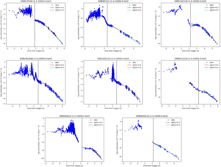
Figure 1. Examples of Swift/XRT X-ray light curves of five LGRBs and three SEEs (blue dots) for which we have high statistics. Red lines show the model of pure dipole radiation with α = 0, while cyan lines show those with α = 0.9. In these plots the magnetar energy release was assumed to be collimated (see Section 6).
Download figure:
Standard image High-resolution imageThe fraction of well fitted systems increases if we introduce a modification to the pure radiating dipole, i.e., by allowing the braking index to be n < 3. The average values of B, k' (see Equation (4)), and P in the different scenarios are summarized in Table 1, where the number of GRBs that could be fit by the corresponding model with spin period P > 0.51 ms (Ngood), as explained in Section 6, is quoted divided by the total number of GRBs analyzed (Ntot). In the case of isotropic NS emission a significant fraction of the LGRBs analyzed show unphysical values of P, below a minimum of 0.51 ms discussed in Section 6. Longer spin periods (all above 0.51 ms) are recovered by assuming a beamed scenario. By assuming an isotropic magnetar the best agreement with the full sample of LGRBs is obtained with α = 0.9, for which statistically acceptable fits were found for 37/40 LGRBs. Assuming ideal magnetic dipole radiation (α = 0), statistically acceptable fits are obtained for 33/40 LGRBs. For the scenario of a beamed magnetar, we find that the best agreement with LGRBs is obtained again by assuming α = 0.9, for which we find statistically acceptable fits for 37/40 LGRBs (Table 2). For an intermediate value of α = 0.3 we found good agreement for 36/40 LGRBs. For the SEEs, statistically acceptable fits are obtained assuming any α and geometry with the exception of GRB 060614, which could be fitted only by assuming α = 0.9, and GRB 130603B, which could be fitted only by assuming α = 0. Contrary to LGRBs, the initial P for SEEs is always found above the minimum value, for both collimated and isotropic energy release from the magnetar.
The best-fit values of B and P of LGRBs plus SEEs in the log–log B–P plane show evidence of a correlation (Figure 2). We compute the Pearson correlation coefficients and the corresponding p-value for the null hypothesis for the sample of LGRBs, SEEs, and LGRBs + SEEs. Results are quoted in Table 1. By fitting our B versus P distribution for the case of a beamed magnetar and α = 0.9 (Figure 2) with a power law we find

where the 1σ error on the slope is computed by taking into account errors on both variables (D'Agostini 2005).
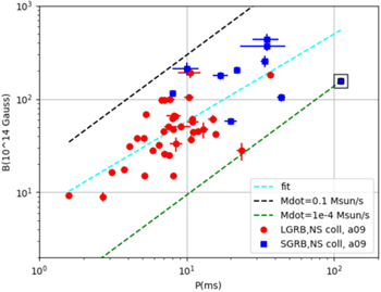
Figure 2. The magnetic field vs. spin period assuming that the spin-down luminosity of the magnetar is entirely beamed within the jet opening angle (data points) for a braking index n = 2.1 (α = 0.9). The long GRBs are marked as red circles while the SEEs are blue squares. Dashed lines indicate the expected B–P relations from accreting NSs for an accretion rate of 0.1 M⊙ s−1 (black) and 10−4 M⊙ s−1 (green) and the best-fit relation (cyan). The framed data point indicates the peculiar "long–short" GRB 060614A.
Download figure:
Standard image High-resolution imageTo test whether SEEs and LGRBs represent distinct populations, as suggested by Dainotti et al. (2017a), we apply a Kolmogorov–Smirnov (KS) test and an Anderson–Darling (AD) test on the obtained B and P distributions for those GRBs with an acceptable fit and with P > 0.51 ms (see next section). Results are quoted in Table 3 and provide robust evidence of two distinct populations.
Table 2. Best-fit Results for the Sample of Long (top) and Short (bottom) GRBs Obtained by Assuming a Magnetar Model with Braking Index n < 3 with α = 0.9, and a Collimated Magnetar
| GRB | t0 | E(t0) | α | k' | B | P | χ2 (d.o.f.) | p-value |
|---|---|---|---|---|---|---|---|---|
| (s) | (1051 erg) | (1014 G) | (ms) | |||||
| 060605 | 157.7 | 0.04 | 0.9 | 1.2 ± 0.1 | 32.4 ± 1.3 | 6.5 ± 0.1 | 48.9(74) | 0.98933 |
| 060607A | ⋯ | ⋯ | ⋯ | ⋯ | ⋯ | ⋯ | ⋯ | ⋯ |
| 060714 | 375.5 | 0.05 | 0.9 | 0.27 ± 0.04 | 50.5 ± 3.5 | 7.5 ± 0.4 | 33.7(44) | 0.86988 |
| 060814 | 660.9 | 0.06 | 0.9 | 0.29 ± 0.03 | 44 ± 2 | 11.1 ± 0.4 | 190.4(169) | 0.12353 |
| 060906 | 262.6 | 0.009 | 0.9 | 0.4 ± 0.1 | 61 ± 6 | 15 ± 1 | 32.2(35) | 0.59990 |
| 060908 | 123.3 | 0.12 | 0.9 | 0.36 ± 0.05 | 191 ± 25 | 10.6 ± 1.9 | 11.3(19) | 0.91099 |
| 061121 | 226.6 | 0.05 | 0.9 | 0.36 ± 0.01 | 47.5 ± 1.3 | 8.1 ± 0.1 | 262.4(254) | 0.34388 |
| 061222A | 193.4 | 0.2 | 0.9 | 0.40 ± 0.02 | 17.7 ± 0.5 | 3.76 ± 0.05 | 399.3(335) | 0.00900 |
| 070208 | 169.6 | 0.001 | 0.9 | 0.5 ± 0.1 | 182 ± 16 | 37 ± 2 | 23.9(31) | 0.81215 |
| 070306 | 457.5 | 0.005 | 0.9 | 1.2 ± 0.1 | 15.0 ± 0.5 | 8.1 ± 0.1 | 164.1(142) | 0.09815 |
| 070318 | 6171.9 | 0.04 | 0.9 | 0.18 ± 0.02 | 28 ± 6 | 23.7 ± 1.8 | 93.4(62) | 0.00603 |
| 070508 | 76.0 | 0.1 | 0.9 | 0.43 ± 0.01 | 97 ± 2 | 7.1 ± 0.1 | 542.5(483) | 0.03121 |
| 070521 | 98.7 | 0.01 | 0.9 | 0.6 ± 0.1 | 65 ± 3 | 8.4 ± 0.2 | 65.7(80) | 0.87562 |
| 070529 | 165.3 | 0.09 | 0.9 | 0.29 ± 0.04 | 99 ± 7 | 7.7 ± 0.6 | 12.65811 (31) | 0.99856 |
| 080310 | 999.3 | 0.02 | 0.9 | 0.6 ± 0.1 | 45 ± 2 | 11.9 ± 0.4 | 59.30765 (67) | 0.73683 |
| 080430 | 374.0 | 0.04 | 0.9 | 0.10 ± 0.01 | 42 ± 2 | 15.7 ± 0.6 | 119.9(142) | 0.909952 |
| 081028A | ⋯ | ⋯ | ⋯ | ⋯ | ⋯ | ⋯ | ⋯ | ⋯ |
| 081029 | 377.7 | 0.04 | 0.9 | 1.8 ± 0.2 | 25 ± 1 | 7.6 ± 0.1 | 71.5(81) | 0.76626 |
| 081221 | 196.3 | 0.2 | 0.9 | 0.40 ± 0.02 | 97 ± 3 | 6.8 ± 0.2 | 268.7(259) | 0.32575 |
| 090205 | 321.5 | 0.02 | 0.9 | 0.5 ± 0.1 | 61 ± 5 | 11.0 ± 0.6 | 18.6(31) | 0.96039 |
| 090418A | 101.7 | 0.01 | 0.9 | 0.7 ± 0.1 | 31 ± 1 | 4.1 ± 0.1 | 7.8(111) | 1.0 |
| 091029 | 471.9 | 0.04 | 0.9 | 0.11 ± 0.01 | 26 ± 1 | 7.1 ± 0.4 | 120.3(130) | 0.71638 |
| 100219A | 464.5 | 0.1 | 0.9 | 1.2 ± 0.3 | 9 ± 1 | 2.7 ± 0.1 | 44.2(26) | 0.014207 |
| 100906A | ⋯ | ⋯ | ⋯ | ⋯ | ⋯ | ⋯ | ⋯ | ⋯ |
| 110213A | 148.4 | 0.02 | 0.9 | 0.89 ± 0.03 | 45.1 ± 0.9 | 7.0 ± 0.1 | 243.8(227) | 0.21048 |
| 110422A | 85.8 | 0.2 | 0.9 | 0.50 ± 0.03 | 62 ± 2 | 8.0 ± 0.1 | 173.4(267) | 1.0 |
| 111008A | 241.8 | 0.1 | 0.9 | 0.29 ± 0.03 | 16.4 ± 0.6 | 3.1 ± 0.1 | 71.9(137) | 1.0 |
| 120118B | 257.4 | 0.004 | 0.9 | 0.2 ± 0.1 | 51 ± 4 | 9.1 ± 1.5 | 8.4(34) | 1.0 |
| 120327A | 163.2 | 0.3 | 0.9 | 0.57 ± 0.04 | 38 ± 2 | 4.6 ± 0.1 | 32.1(59) | 0.99832 |
| 120404A | 438.3 | 0.08 | 0.9 | 0.6 ± 0.1 | 66 ± 4 | 8.2 ± 0.9 | 17.5(36) | 0.99604 |
| 120521C | 650.5 | 0.06 | 0.9 | 0.4 ± 0.1 | 33 ± 6 | 8.5 ± 0.8 | 0.5(6) | 0.99764 |
| 120811C | 216.4 | 0.1 | 0.9 | 0.40 ± 0.07 | 38 ± 3 | 5.1 ± 0.2 | 32.2(46) | 0.93796 |
| 120907A | 90.3 | 0.04 | 0.9 | 0.11 ± 0.02 | 104 ± 6 | 10.4 ± 0.8 | 66.3(87) | 0.95166 |
| 120922A | 657.8 | 0.05 | 0.9 | 0.40 ± 0.05 | 37 ± 4 | 10.7 ± 0.4 | 21.8(70) | 0.999999 |
| 121128A | 127.1 | 0.3 | 0.9 | 0.48 ± 0.04 | 68 ± 5 | 5.3 ± 0.1 | 67.0(90) | 0.966758 |
| 131105A | 327.8 | 0.04 | 0.9 | 0.12 ± 0.02 | 57 ± 4 | 11 ± 1 | 16.3(50) | 1.0 |
| 131117A | 312.3 | 0.1 | 0.9 | 0.21 ± 0.03 | 47 ± 9 | 13 ± 1 | 0.36(11) | 1.0 |
| 140206A | 411.38 | 1.0 | 0.9 | 0.48 ± 0.02 | 9.3 ± 0.2 | 1.59 ± 0.02 | 315.6(442) | 1.0 |
| 140506A | 573.5 | 0.4 | 0.9 | 0.17 ± 0.02 | 15 ± 1 | 5.2 ± 0.2 | 88.8(140) | 0.999763 |
| 140512A | 326.9 | 0.2 | 0.9 | 0.51 ± 0.01 | 28 ± 1 | 5.9 ± 0.1 | 325.8(363) | 0.920167 |
| 051221A | 1868.9 | 0.002 | 0.9 | 0.25 ± 0.05 | 104 ± 9 | 44 ± 3 | 62.1(47) | 0.06815 |
| 060614A | 1630.5 | 3.3e–06 | 0.9 | 1.3 ± 0.1 | 156 ± 5 | 111 ± 1 | 151.5(140) | 0.23827 |
| 060912A | 143.5 | 0.01 | 0.9 | 0.13 ± 0.03 | 435 ± 65 | 35 ± 7 | 43.0(33) | 0.11397 |
| 061201 | 9.8 | 0.02 | 0.9 | 0.9 ± 0.1 | 206 ± 15 | 22 ± 0.7 | 29.8(24) | 0.19257 |
| 070714B | 572.1 | 0.01 | 0.9 | 0.8 ± 0.2 | 369 ± 40 | 35 ± 12 | 39.0(20) | 0.00629 |
| 070809 | 497.9 | 0.002 | 0.9 | 0.3 ± 0.1 | 58 ± 11 | 20 ± 2 | 16.4(13) | 0.23016 |
| 070810A | 167.8 | 0.01 | 0.9 | 0.4 ± 0.1 | 178 ± 17 | 17 ± 2 | 7.0(29) | 0.99999 |
| 090426 | 1.5 | 0.01 | 0.9 | 0.10 ± 0.05 | 212 ± 33 | 10 ± 2 | 13.8(27) | 0.982628 |
| 090510 | 1.4 | 0.02 | 0.9 | 1.0 ± 0.1 | 116 ± 5 | 8 ± 0.1 | 83.4(70) | 0.13127 |
| 100724A | 55.7 | 0.01 | 0.9 | 0.4 ± 0.1 | 255 ± 38 | 34 ± 2 | 11.9(15) | 0.68291 |
| 130603B | ⋯ | ⋯ | ⋯ | ⋯ | ⋯ | ⋯ | ⋯ | ⋯ |
Download table as: ASCIITypeset image
Table 3. Results from the KS and AD Tests
| NS Isotropic | NS Collimated | ||||||||||
|---|---|---|---|---|---|---|---|---|---|---|---|
| Distribution | α | Ngood/Ntot | KS | p-value | AD | Sign. | Ngood/Ntot | KS | p-value | AD | Sign. |
| B | 0.0 | 29/51 | 0.84 | 5 × 10⁻⁵ | 11.2 | 7 × 10⁻⁵ | 43/51 | 0.78 | 6 × 10⁻⁵ | 11.3 | 7 × 10⁻⁵ |
| P | 0.0 | 29/51 | 0.74 | 6 × 10⁻⁴ | 8.9 | 2 × 10⁻⁴ | 43/51 | 0.71 | 3 × 10⁻⁴ | 10.3 | 1 × 10⁻⁴ |
| B | 0.9 | 36/51 | 0.92 | 2 × 10⁻⁶ | 13.7 | 3 × 10⁻⁵ | 47/51 | 0.82 | 1 × 10⁻⁵ | 13.5 | 3 × 10⁻⁵ |
| P | 0.9 | 36/51 | 0.81 | 5 × 10⁻⁵ | 11.8 | 6 × 10⁻⁵ | 47/51 | 0.74 | 1 × 10⁻⁴ | 10.1 | 1 × 10⁻⁴ |
Note. The tests were applied on the distribution of B and P for the LGRB + SEE sample. The second column quotes the values assumed for the braking index function α (see Section 2). The third column quotes the number of GRBs that could be fit by the corresponding model with spin period P > 0.51 ms (Ngood), as explained in Section 6, divided by the total number of GRBs analyzed (Ntot). The KS statistics with the associated chance probability and the AD statistics with the associated significance level (an approximate significance level at which the null hypothesis for the provided samples can be rejected) are quoted for different assumptions on the magnetar model.
Download table as: ASCIITypeset image
A GRB worth mentioning is GRB 060614, which has properties of both an LGRB and an SGRB. Indeed, it is placed among the SEE population in the B–P plane, further confirming its links to SGRB progenitors.
6. Discussion
6.1. Validity of the Magnetar Scenario
We tested whether the magnetar model was consistent with all GRBs in our sample, and obtained accurate fits to the X-ray light curves for (90%) of our selected plateaus. Besides the successful fits, we checked the consistency of the resulting parameters with physical constraints on NS properties, in particular its maximum spin energy. The latter is set by the equation of state (EoS) of matter at supranuclear density, and depends on the NS mass and radius. It is ≲3 × 1052 erg for a "standard" NS, with a mass ∼1.4 M⊙ and a radius of 12 km, for which the minimum spin period is ≈1 ms (Bucciantini et al. 2007, 2009; Duffell et al. 2015; Lattimer 2016). However, in more massive (≳2.1 M⊙) and compact (R ≈ 10 km) NSs, the maximum spin energy can reach up to ∼1053 erg (e.g., Dall'Osso et al. 2018 and references therein). Since in our fits we have assumed a fiducial NS with a mass of 1.4 M⊙ and radius of 12 km, a spin energy of 1053 erg would correspond to an effective minimum spin period of 0.51 ms. Thus, all spin periods >0.51 ms up to ∼1.0 ms obtained in our fits are considered to be consistent with an NS central engine having a different mass and/or radius than the fiducial values.
An additional source of uncertainty in the energy budget of the magnetar is the degree of anisotropy of its spin-down luminosity (Section 2).
The spin-down energy of a millisecond NS is carried away by a Poynting-flux/electron–positron wind, which is expected to be launched in a near-isotropic fashion (e.g., Usov 1992; Fan & Xu 2006; Metzger & Piro 2014). However, if the magnetar is born at the center of a collapsar, the progenitor star could cause a collimation of the emitted energy, during both the prompt phase (Bucciantini et al. 2007, 2009; Duffell et al. 2015) and the afterglow phase (Lü & Zhang 2014). Mazzali et al. (2014) argue for the magnetar wind to be close to isotropic in collapsars based on the energetics of the associated supernovae and on the assumption that the maximum spin energy of an NS is ∼2 × 1052 erg. However, as pointed out above, the whole range of possible spin energy values leaves room for non-negligible beaming even in this case.
This is also indicated by recent detailed numerical simulations of proto-magnetar (PM) formation (Obergaulinger & Aloy 2017). This study strongly suggests that (1) the formation of a PM is preceded by the ejection of a highly collimated outflow, (2) the environment surrounding the PM is highly anisotropic, with a large variation in properties from the direction of the rotational axis to the equatorial region, and (3) the maximum rotational energy that may be stored (and hence constitutes the energy reservoir for the magnetar spin-down) can be significantly larger than previously suggested limits and consistent with the values adopted here (see above). Both the collimated ejecta and the anisotropy of the medium surrounding the PM may certainly have an impact on the observed distribution of the spin-down energy. This provides a possible interpretation as to why our fits suggest a preference for a collimated spin-down.
Table 1 shows that, for the isotropic and ideal case, 18 out of 40 LGRBs cannot provide an acceptable fit, mostly because they would require an unphysically short NS spin period, indicating a clear preference for a non-isotropically emitting magnetar, and a non-ideal spin-down model (i.e., n < 3). By assuming that the magnetar collimation is the same as the afterglow one, for the case with α = 0.9 only four out of 51 systems are not well fitted, and all of them have P > 0.51 ms. We note that this result continues to be valid even for a milder degree of collimation, and for intermediate values of α.
6.2. The Correlation of B versus P and the Anticorrelation of  versus P

The most novel finding of our work is that, independent of the assumed particular magnetar parameters (i.e., collimation and braking index), there is evidence for a statistically significant correlation in the B versus P plane for all GRBs in our sample. A B–P correlation is expected from the well-established physics of the spin-up line for accreting NSs in Galactic binary systems. For a given  , the NS reaches an equilibrium period Peq ∝ B6/7 (e.g., Bhattacharya & van den Heuvel 1991; Pan et al. 2013).
For the fixed values of M and R used in our fits, we find that all our data in the B–P plane are encompassed by two lines corresponding to the range of mass accretion rates 10−4 M⊙ s−1  . In other words, the normalization of the B–P relation obtained here perfectly matches spin-up line predictions for the magnetar model with mass accretion rates expected in the GRB prompt phase (see, e.g., Bernardini 2015 and references therein). The latter are ∼11–14 orders of magnitude higher than those inferred for accreting NSs, where this physics was originally derived. Thus, it appears that the same basic physics is at play, but in powering a GRB, the accretion rates grow substantially because they are not the result of a companion shedding a fraction of its mass on a secular timescale, but rather of a progenitor being swallowed whole by the nascent magnetar.
Thus, the presence of a correlation in the B–P plane of our parameters fitted to the X-ray light curve, with a slope consistent with that of Equation (8), serves as a clue that leads us to explore the spin-up line physics of Galactic millisecond pulsars in the context of GRBs. The correlation is necessarily noisy due to the presence of a variety of opening angles and a range of radii, masses, and detailed magnetic physics across the sample. The strong result is the bounding of the B–P parameters between two limiting values of  that are those expected in the context of GRBs.
Interestingly, SEEs systematically populate the long-period end of the distribution, while the LGRBs appear to have systematically faster spins (and lower B-fields). This evidence can be interpreted in a way that is consistent with the expectations from the spin-up limit if SEEs are associated with progenitors that yield, on average, a smaller amount of accretion material than LGRB progenitors, e.g., binary NS mergers as opposed to collapsars. Indeed, the total accreted mass (ΔM) determines the position of a millisecond pulsar in the B–P diagram (Pan et al. 2013), a greater ΔM corresponding to a larger transfer of angular momentum and thus a shorter spin period of the nascent magnetar.
We have shown that the X-ray afterglow light curves can be fully described using a set of four parameters (k, E, B, P). The latter two, which are related to the neutron star properties, are also correlated, as shown in Figure 2. This provides a physical foundation for the Dainotti 2D relation between La and Ta. This correlation carries its own intrinsic scatter, as expected from the spread in the B–P plane, which is only partially due to an intrinsic spread in the mass and radii of the neutron star, but mostly due to a spread in the mass accretion rates. Thus, a clear link between the X-ray afterglow and the prompt energetics is established, as  is the key physical parameter in determining the luminosity during the prompt phase. This last in turn explains the 3D Dainotti relation where the parameters of the X-ray afterglow are linked to the prompt Lpeak; at fixed opening and viewing angles, and fixed mass and radius of the NS,
  determines Lpeak and, together with the initial magnetic field, fixes the position of the nascent magnetar along the particular spin-up line, which then determines the resulting X-ray afterglow light curve.
If  can be considered as a proxy for the luminosity in the prompt phase (Lpeak), our result provides a natural connection between the properties of the plateaus and those of the prompt emission in GRBs. Observationally, one such correlation has been identified by Dainotti et al. (2017a). Additionally, we would expect an anticorrelation between P and Lpeak. We found a weak indication of such an anticorrelation (the Pearson correlation coefficient is only −0.33), with a trend given by Lpeak ∝ P−0.27. However, due to the paucity of the data no definite conclusion can be drawn. Further work on this is currently under way and will be the subject of a subsequent publication.
7. Conclusions
In this work we analyze the plateau phase observed in the X-ray afterglows of two homogeneous samples of GRBs (LGRBs and SEEs) in the context of the magnetar paradigm, taking into account two angular patterns for the magnetar energy release (i.e., collimated versus isotropic) and different values of the braking index n. The afterglow light curves can be accurately reproduced for the vast majority of our sample. The distributions of the best-fit values of the magnetic field strengths B and the spin periods P for the samples of SEEs and LGRBs are consistent with originating from two distinct populations. The evidence for SEEs constituting a separate population was first obtained by Dainotti et al. (2017b) on more empirical grounds. The confirmation of the existence of two distinct GRB populations also on a physical basis has fundamental implications for the use of the GRB correlations as cosmological tools, in the efforts toward a general standardization of these sources (see Dainotti et al. 2016, 2018; Dainotti & Del Vecchio 2017), and the study of selection effects (Dainotti & Amati 2018).
It is extremely interesting that the magnetar parameters we find, when plotted in a B–P diagram, are neatly encompassed by the well-known spin-up line physics of B ∝ P7/6 of Galactic millisecond pulsars. This, for typical NS masses ≈1.4 M⊙ and radii ≈12 km, requires mass accretion rates  , typically expected in GRBs, which are about 11–14 orders of magnitude larger than typical in accreting pulsars. Thus, it appears that the same basic physics is at play even in the huge mass accretion rate that powers GRBs.
We see LGRBs systematically requiring shorter periods, as expected from a larger total accreted mass resulting in more transfer of angular momentum than for the SEE GRBs. This is consistent with interpreting the period of the magnetar as being fixed by the spin-up line, and also with our independent discovery of SEEs and LGRBs being distinct populations. The B–P correlation is robust since it is independent of specific assumptions made on details on the magnetar spin-down. The collimation factor and the braking index mostly shift the resulting B versus P distribution parallel to the spin-up line. Our study therefore strongly supports the origin of the X-ray plateaus being the magnetar central engine.
M.G.D. acknowledges the initial support of the Marie Curie Program, because the research leading to these results has received funding from the European Union Seventh Framework Program (FP7-2007/2013) under grant agreement no. 626267 and the current support of the American Astronomical Society through the Chretienne Fellowship. S.D. acknowledges support from NSF award AST-1616157. X.H. acknowledges financial assistance from UNAM DGAPA grant IN104517 and CONACyT. G.S. acknowledges EGO support through a VESF fellowship (EGO-DIR-133-2015). This work made use of data supplied by the UK Swift Science Data Centre at the University of Leicester.
Facility: Swift (XRT and BAT). - Swift Gamma-Ray Burst Mission
Footnotes
- 8
A braking index n > 3 for a newborn NS is possible if additional energy losses, e.g., gravitational wave emission, contribute to its spin-down. We note that n > 3 has also been suggested for old pulsars.
- 9
- 10