Abstract
We use Interstellar Boundary Explorer (IBEX) measurements of energetic neutral atoms (ENAs) to constrain the proton (mostly pickup ion, PUI) distribution in the heliotail. In our previous study, we solved the Parker transport equation and found that the velocity diffusion coefficient D(v) for PUIs is approximately D(v) ∼ 1.1 × 10⁻⁸ km2 s−3 (v/v0)1.3, assuming the initial proton distribution processed by the termination shock (TS), fp,0, is a kappa distribution with kappa index κp,0 = 1.63. In this study, we test different forms for fp,0. We find that if fp,0 is kappa-distributed and D(v) = D0(v/v0)1.3, any kappa index in the range 1.5 < κp,0 < 10 is consistent with IBEX data if D0 ∼ 0.8–1.3 × 10⁻⁸ km2 s−3. While the case where D(v) ∝ v1.3 yields ENA fluxes that appear to best reproduce IBEX data for any κp,0, it is possible for D(v) to scale close to ∼v2/3 or ∼v2 within our uncertainties by changing D0. We also show that an upstream PUI filled-shell distribution that is heated by a quasi-stationary TS, generating a downstream filled-shell with large cutoff speed, yields an excess of ENAs >2 keV compared to IBEX. However, using a fully kinetic particle-in-cell simulation to process a PUI filled-shell across the TS yields ENA spectra consistent with IBEX, reinforcing the significance of self-consistent, preferential PUI heating and diffusion at the TS. Interestingly, an upstream PUI distribution inferred from the particle-in-cell simulation to reproduce Voyager 2 observations of the nose-ward TS is inconsistent with IBEX observations from the heliotail, suggesting differences in the upstream PUI distribution or TS properties.
Export citation and abstract BibTeX RIS
1. Introduction
The Interstellar Boundary Explorer (IBEX; McComas et al. 2009a) is an Earth-orbiting spacecraft that measures neutral atom fluxes coming from the outer heliosphere (McComas et al. 2009b). IBEX detects neutral atoms from the very local interstellar medium (VLISM; Möbius et al. 2009; Bochsler et al. 2012; Rodríguez Moreno et al. 2013; McComas et al. 2017a), and also energetic neutral atoms (ENAs) produced by charge exchange between solar wind (SW) ions and interstellar neutral atoms in the heliosphere (Gruntman et al. 2001; Heerikhuisen et al. 2008; Prested et al. 2008; McComas et al. 2009b; Zank 2015). The hydrogen ENA fluxes observed by IBEX inform us of how the solar and interstellar plasmas interact with neutral atoms in different regions of the heliosphere, as well as the structural size and shapes of the distant heliosphere boundaries (e.g., Zank 1999, 2016; Zirnstein et al. 2018a).
IBEX observations of ENAs from the hot inner heliosheath (IHS), in particular, have revealed the importance of pickup ions (PUIs) in modifying the plasma pressure in the heliosheath. A significant number of PUIs are created in the supersonic SW from charge exchange between the fast SW ions and cold interstellar neutral atoms flowing in from the VLISM. PUIs are quickly scattered in pitch angle and advect with the bulk motion of the SW. Beyond ∼20 au from the Sun, PUIs already constitute a few percent of the total proton number density and most of the internal particle pressure (McComas et al. 2017b). At distances near the TS (∼100 au from the Sun), the relative PUI-to-SW ion density is expected to be ∼15%–30%. Voyager 2 observations (Richardson et al. 2008) suggest that PUIs are preferentially heated at the TS (see also Chalov & Fahr 1996; Zank et al. 1996, 2010; Yang et al. 2015; Kumar et al. 2018). Thus, PUIs contain the majority of IHS plasma pressure (e.g., Livadiotis et al. 2013), and are responsible for a significant number of ∼0.5–6 keV ENAs observed by IBEX (e.g., Desai et al. 2014; Zirnstein et al. 2014). However, understanding the plasma in the heliotail is particularly complicated, since (1) we do not have any in situ observations in the heliotail, (2) the charge-exchange process preferentially removes energetic protons (below ∼20 keV) and injects low energy PUIs over long timescales, significantly modifying the distribution (e.g., Zirnstein et al. 2017, 2018b), and (3) the heliosphere modeling community is not in agreement regarding the shape and structure of the heliotail (e.g., Izmodenov & Alexashov 2015; Opher et al. 2015; Pogorelov et al. 2015; Dialynas et al. 2017; Schwadron & Bzowski 2018). Thus, studies focused on the production and transport of PUIs, and their role in forming ENA spectra observed by IBEX are needed to better understand the properties of the heliotail.
In our previous work (Zirnstein et al. 2018b), we developed a model for the transport of SW ions and PUIs in the heliotail to understand the origin of the IBEX ENA spectrum (Figure 1) and the importance of velocity diffusion of PUIs in the heliotail. We found that, in order to reproduce IBEX ENA observations, some form of stochastic diffusion of ∼0.1–5 keV PUIs must be occurring in the IHS. Assuming that the proton distribution function (including SW ions and PUIs) downstream of the TS is a kappa distribution with index 1.63, we derived a best-fit diffusion coefficient amplitude (D0) of ∼1.1 × 10⁻⁸ km2 s−3 and velocity spectral dependence (γ) of ∼1.25, where the diffusion coefficient is of the form D(v) = D0 (v/v0)γ and v0 = 1 km s−1. We found that velocity diffusion mechanisms with spectral indices above ∼2 or below ∼2/3 are not likely, suggesting that the most likely diffusion coefficient lies between the coefficients predicted by particle resonant interactions with the well-known incompressible MHD turbulence spectra, isotropic Kolmogorov (D(v) ∝ v2/3; e.g., Isenberg 1987) and anisotropic Goldreich–Sridhar turbulence (D(v) ∝ v2; e.g., Eichler 2014), or particle interactions with compressive fluctuations in the SW (D(v) ∝ v2; e.g., le Roux et al. 2005; Zhang & Lee 2013).
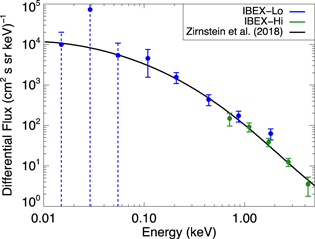
Figure 1. ENA fluxes from the heliotail observed by IBEX from 2009 to 2012 during low solar activity (Galli et al. 2017). Note that the lowest three data points are consistent with zero flux and have large uncertainties (dashed lines). We do not include these data points in our analyses. Also shown is a model ENA spectrum from Zirnstein et al. (2018b) that was produced by solving the Parker transport equation with charge-exchange source terms and velocity diffusion.
Download figure:
Standard image High-resolution imageHowever, Zirnstein et al. (2018b) did not test the effects of the proton distribution boundary condition in detail, namely the form of the distribution function processed by the TS. While these authors demonstrated that the model ENA spectrum only slightly changes when the kappa index is varied, this was tested only for a single diffusion rate. A different initial distribution function may require changing the diffusion rate applied in the heliotail in order to best reproduce IBEX observations. In this study, we expand on our previous work by analyzing the effects of the initial proton distribution function downstream of the TS in the heliotail (i.e., the inner boundary condition) on ENA fluxes measured at 1 au. We utilize the transport model developed in our previous work, while varying both the initial proton distribution function and the diffusion coefficient, to calculate the ENA spectrum at 1 au produced from our model and compare to IBEX ENA observations from the heliotail.
2. Model of Proton Distribution in the IHS
2.1. Transport Equation
Following the work of Zirnstein et al. (2018b), we solve the stationary Parker transport equation with charge-exchange source terms, including (1) the advection of PUIs with the bulk plasma, (2) the adiabatic heating of the plasma derived from our 3D MHD/kinetic model of the heliosphere, and (3) a velocity diffusion term that is left as a free parameter. The transport equation is given as
where v is the proton speed in the plasma frame, up is the bulk flow speed along the streamline distance coordinate s, fp is the isotropic proton distribution function, D(v) is the velocity diffusion coefficient, which we assume is a free parameter,  is the bulk plasma flow divergence, P is the production (source) term due to charge exchange (photoionization is negligible, and electron-impact ionization is ignored), and L is the loss (sink) term due to charge exchange with neutral hydrogen atoms. As in our previous work, the plasma flow speed, flow divergence, and neutral hydrogen distribution used to calculate the charge-exchange source terms are taken from our MHD-plasma/kinetic-neutral simulation of the heliosphere (Zirnstein et al. 2016). The velocity diffusion coefficient is written in the form D(v) = D0 (v/v0)γ, where D0 is the diffusion rate amplitude with units km2 s−3, γ is the velocity spectral index, v is the particle speed, and v0 = 1 km s−1 is a normalization speed. Following prior works (e.g., Chalov et al. 2003; Fahr & Scherer 2004; Chalov et al. 2016), we assume that the spatial diffusion time of ∼keV PUIs is much larger than their advection time with the bulk plasma flow in the IHS.
The charge-exchange source terms are given by (see Zirnstein et al. 2018b for details)

Equations (2) and (3) are derived by assuming that the proton distribution function is isotropic in the plasma frame; therefore, we integrate over solid angle in velocity space (see also Malama et al. 2006). Equation (3) is further simplified by the fact that the majority of neutral hydrogen atoms in the heliotail are (1) interstellar neutral atoms from the VLISM and (2) neutral atoms that are produced by charge exchange in the slowed and compressed outer heliosheath (OHS), where both populations are approximately Maxwell–Boltzmann (e.g., Izmodenov 2001; Heerikhuisen et al. 2006). It is important to include the second population since these neutral atoms continue to enter the heliotail from outside the heliopause for long distances from the Sun. Thus, by assuming these two neutral populations are Maxwell–Boltzmann, the charge-exchange loss term can be written in the form of Equation (3), where the double integral has an analytic solution (see Equation (7) of Zirnstein et al. 2018b). The method for solving Equation (1) is briefly summarized in the Appendix, and more details can be found in Zirnstein et al. (2018b).
2.2. Proton Distribution Downstream of the TS
The purpose of this study is to test different initial proton distribution functions downstream of the TS and analyze their effects on the evolution of the distribution in the heliotail and on ENA fluxes at 1 au. We test three analytic forms for the initial proton distribution function (fp,0) and one distribution extracted from a particle-in-cell (PIC) simulation of the TS. The three analytic functions are (1) a single kappa function representing the entire proton distribution, while varying the kappa index, (2) a superposition of a Maxwell–Boltzmann distribution representing the core SW ions and a filled-shell distribution (Vasyliunas & Siscoe 1976) for PUIs, and (3) a superposition of three Maxwell–Boltzmann distributions representing core SW ions, PUIs that are transmitted across the TS, and PUIs that are singularly reflected at the TS, then transmitted (Zank et al. 2010). The analytic distributions and their properties are described in Table 1. In Section 4.3, we describe the PIC simulation results.
Table 1. Parameters for the Initial Proton Distribution Functions Downstream of the TS
| Distributions | Parameters (units) | Value |
|---|---|---|
| Kappa, fκ | Density, np,0 (cm−3) | 0.0017a |
| Temperature, Tp,0 (K) | 1.9 × 10⁶a | |
| Kappa index, κp,0 | 1.5–10 | |
| Maxwell–Boltzmann + Filled Shell, fMS | PUI density fraction, α | 0.25 |
| TS compression ratio, r | 3a | |
| Upstream SW flow speed, up,u (km s−1) | 350 | |
| Upstream core SW temperature, Tp,u (K) | 104b | |
| Three Maxwell–Boltzmann, f3M | Reflected PUI density fraction, β | 0.08c |
| Core SW temperature, Tp,SW (K) | 1.0 × 10⁵c | |
| Transmitted PUI temperature, Tp,tr (K) | 4.1 × 10⁶c | |
| Reflected PUI temperature, Tp,ref (K) | 4.4 × 10⁷c | |
Notes.
aDerived from our MHD simulation (Zirnstein et al. 2016). bTaken from Voyager 2 observations upstream of the TS (Richardson et al. 2008). cDerived from models of Chalov & Fahr (1996) and Zank et al. (2010).Download table as: ASCIITypeset image
First, we use a kappa distribution of the form (e.g., Livadiotis & McComas 2013)
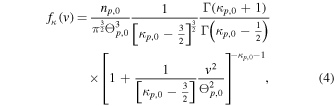
with initial density np,0, temperature Tp,0, kappa index κp,0, and characteristic speed  . The initial density and temperature are assumed to be 0.0017 cm−3 and 1.9 × 10⁶ K, which are taken from our MHD simulation (i.e., downstream of our simulated TS in the VLISM downwind direction; Zirnstein et al. 2016). We vary the kappa index in the range 1.51 ≤ κp,0 ≤ 10. We note that the variable κp,0 here is equivalent to the 3D kappa index from Livadiotis & McComas (2013), not their invariant kappa index.
The second distribution that we test is a combination of a Maxwell–Boltzmann distribution for the core SW ions and a filled-shell distribution for PUIs (i.e., Vasyliunas & Siscoe 1976) that is compressed at the TS. Upstream of the TS (subscript "u"), the proton distribution is
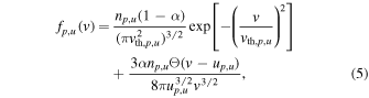
where np,1 is the total upstream proton density, α is the PUI density fraction (assumed to be 25%; e.g., see Figure 2 in Zirnstein et al. 2017), up,u = 350 km s−1 is the upstream SW speed, and vth,p,1 is the upstream thermal velocity of the core SW (assumed to have a temperature of 104 K, similar to that observed by Voyager 2 upstream of the TS; Richardson et al. 2008). Following Zank et al. (2010), we derive the downstream proton distribution by transporting the upstream distribution across the TS under the assumption that the particles and bulk flow are decelerated by the cross-shock potential, yielding the downstream particle speed (in the flow frame) to be vd = rvu (see Zank et al. 2010 for more details), where r = 3 is the shock compression ratio. Using Liouville's theorem, we derive the downstream proton distribution fp,d in terms of the upstream distribution fp,u as
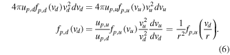
This yields the downstream proton distribution:
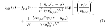
Since np,0 is the total proton density downstream of the TS, then r × np,u = np,d = np,0. Thus, Equation (7) can be rewritten as
The initial proton distribution parameters for Equation (8) are shown in Table 1, which are taken from our 3D MHD simulation of the heliosphere (Zirnstein et al. 2016).
The third distribution that we test is a superposition of three Maxwell–Boltzmann functions, representing (1) the core SW ions, (2) PUIs transmitted across the TS, and (3) PUIs reflected and then transmitted across the TS. This composite distribution is commonly used to model multicomponent ion species in the heliosheath (e.g., Zank et al. 2010; Zirnstein et al. 2014, 2017; Swaczyna & Bzowski 2017a; Swaczyna et al. 2017b). Unlike the case where we process the filled-shell distribution across the TS, here we simply assume that the downstream distribution is represented by three Maxwell–Boltzmann distributions with total density np,0 and effective temperature Tp,0. Following Zank et al. (2010), we directly write the downstream distribution f3M as
where α is the PUI density fraction (25%), β is the fraction of PUIs that are reflected at the TS (8%; Zank et al. 2010; Chalov & Fahr 1996), and vth,p,SW, vth,p,tr, and vth,p,ref are the initial thermal speeds of core SW ions, transmitted PUIs, and reflected PUIs, respectively ( ). We choose the thermal speeds (i.e., temperatures) for each component such that their total thermal pressure satisfies the thermal pressure given by our MHD simulation downstream of the TS, np,0kBTp,0,
where np,0 = 0.0017 cm−3, Tp,0 = 1.9 × 10⁶ K, and the temperature fractions Γp,SW = Tp,SW/Tp,0, Γp,tr = Tp,tr/Tp,0, and Γp,ref = Tp,ref/Tp,0. Knowing their thermal pressure fractions (Table 1; see also Zank et al. 2010; Zirnstein et al. 2017), the initial temperature of each component is Tp,SW = 1.0 × 10⁵ K, Tp,tr = 4.1 × 10⁶ K, and Tp,ref = 4.4 × 10⁷ K.
Examples of each distribution (Equations (4), (8), and (9)) are shown in Figure 2 for the same total density and temperature (for the kappa distribution, we show several cases for κp,0). Using these distributions as initial boundary conditions, we solve the Parker transport equation (Equation (1)) for a range of velocity diffusion coefficients. In the following sections, we compute ENA fluxes at 1 au from the model proton distributions and provide a quantitative comparison with IBEX data to determine their physical likelihood.
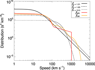
Figure 2. Initial proton distribution functions downstream of the TS used in our analysis: (1) kappa distribution (fκ, here we show several cases for the kappa index), (2) Maxwell–Boltzmann for the core SW and filled-shell for PUIs (fMS), and (3) three Maxwell–Boltzmann distributions for core SW, transmitted PUIs, and reflected PUIs (f3M).
Download figure:
Standard image High-resolution image3. Results: Evolution of the Proton Distribution in the Heliotail
Figure 3 shows examples of the evolution of the proton distribution, assuming fp,0 is (1) a kappa distribution (fκ) with κp,0 = 1.63, (2) a Maxwell–Boltzmann plus filled-shell distribution (fMS), and (3) a superposition of three Maxwell–Boltzmann distributions (f3M). It is clear that, while each distribution is different near the TS (also see Figure 2), after a few hundred astronomical units they evolve toward nearly the same shape. This is due to the velocity diffusion term, which diffuses particles in energy until they approach a common spectrum. The first case (fκ) does not significantly change with distance in the range ∼100–1000 km s−1, as originally pointed out by Zirnstein et al. (2018b), although the distribution does slowly decrease in density at higher speeds due to energy-dependent, charge-exchange losses (Lindsay & Stebbings 2005). After traveling ∼300 au from the TS, the plasma compresses in the simulation heliotail, whose effects are introduced into the solution of Equation (1) through the flow divergence term  . Adiabatic compression and heating significantly affects the distribution at low speeds (<100 km s−1). The sharp features in the other two initial distributions in Figures 3(b) and (c) (fMS and f3M) eventually smooth and broaden in energy within ∼400 au of the TS and are also compressed and heated at low and high speeds where the charge-exchange loss rate is ineffective compared to adiabatic heating.

Figure 3. Evolution of the proton distribution assuming three different initial distributions from Figure 2, and the same velocity diffusion coefficient D(v) = 1.125 × 10⁻⁸ [km2 s−3] × (v/v0)1.25. The initial distribution downstream of the TS is plotted in black. The distribution at larger distances from the TS are plotted according to the color bar.
Download figure:
Standard image High-resolution imageWe are particularly interested in the range of speeds that coincide with the energies at which IBEX observes ENAs, which is ∼50 eV to 5 keV in the solar inertial frame (see Figure 1). Converting these energies to the receding plasma frame (assuming it is moving away from the Sun on average ∼50 km s−1, see Zirnstein et al. 2018b, Figure 8) gives a range of speeds ∼100–1000 km s−1. Figure 3 shows that, in this range, the distributions are initially quite different, but eventually they evolve toward similar shapes after a few hundred astronomical units from the TS. It is important to understand how the proton distribution evolves with distance, because this affects the ENA spectrum observed by IBEX, which is a line-of-sight integration of ENAs produced in the heliosheath. By converting the proton distributions to ENA fluxes at 1 au and comparing to IBEX data, we may be able to infer which distributions are realistic and gain insight into how PUIs are transmitted across the TS.
4. Results: ENA Fluxes at 1 au
We calculate the line-of-sight integrated ENA flux at 1 au from the proton distributions illustrated in the previous section (with different initial conditions and velocity diffusion coefficients) similar to the method in our previous works (e.g., Zirnstein et al. 2013, 2017, 2018b, and references therein). The calculations are performed in the solar inertial frame, and we account for losses of ENAs as they travel from their point of creation inside the heliotail to the TS, but not in the supersonic SW. Finally, before comparing to IBEX data, we smooth the model ENA spectrum over energy using a Gaussian function with full-width at half-maximum ΔE/E = 0.7, emulating the energy response function of the IBEX instruments (Funsten et al. 2009; Fuselier et al. 2009). We compare to IBEX ENA data extracted from a group of pixels centered on the VLISM downwind direction (see Figure 1). The data are weight-averaged over time from 2009 to 2012 during a period of low solar activity, converted to the solar inertial frame, and are corrected for ENA losses within 100 au of the Sun (see Galli et al. 2017 for more details).
4.1. Dependence on the Kappa Distribution Index
In this section, we analyze how the diffusion coefficient in the heliotail and model ENA spectrum at 1 au depend on the initial proton distribution assuming it is a kappa function (the first of three cases, see Equation (4)). Figure 4 shows model ENA fluxes assuming that fp,0 is a kappa distribution for a selection of kappa index values in the range 1.51 ≤ κp,0 ≤ 10. Figure 4(b) shows the case where the velocity diffusion coefficient is close to the best fit derived by Zirnstein et al. (2018b) for κp,0 = 1.63. For small κp,0 (1.51) the resulting ENA spectrum is lower than those with larger proton kappa indices. While one might expect to see more high energy ENAs from a proton distribution with a small kappa index, protons in a κp,0 ∼ 1.5 distribution are at much higher energies than what IBEX can observe. A distribution with 5 < κp,0 < 10 actually produces the most ENAs observable by IBEX in the ∼0.1–5 keV energy range.
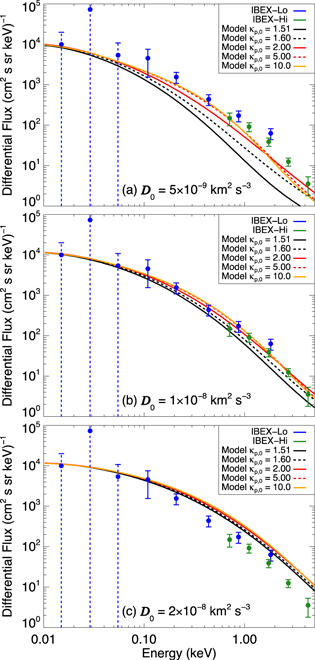
Figure 4. Model ENA fluxes assuming a kappa distribution for fp,0, with different kappa indices κp,0. We assume the diffusion coefficient D(v) ∝ v1.25 and vary the diffusion amplitude, D0.
Download figure:
Standard image High-resolution imageDepending on the diffusion rate, ENA spectra resulting from proton distributions with different κp,0 can significantly deviate from each other at energies >0.5 keV, suggesting that different diffusion rates are required to best fit IBEX data. Figure 4(a) shows that if the diffusion rate amplitude D0 was slightly lower (∼5 × 10⁻⁹ km2 s−3), then it would appear that a larger kappa index would be needed to better match IBEX data; however, in this case none of the spectra can reproduce the entire IBEX spectrum. On the other hand, a larger diffusion coefficient amplitude (D0 ∼ 2 × 10⁻⁸ km2 s−3; Figure 4(c)) would produce similar ENA spectra regardless of κp,0, all of which overestimate IBEX measurements. The relationship between κp,0 and D0 is illustrated in more detail in the left panel of Figure 5, which shows the reduced chi-square values between the model and IBEX data as a function of κp,0 and D0, setting γ = 1.25. Figure 5 shows a broad region of reduced chi-square less than or equal to 1 when κp,0 ≲ 7 and 8 × 10⁻⁹ km2 s−3 ≲ D0 ≲ 1.3 × 10⁻⁸ km2 s−3. As κp,0 approaches 1.5, a significantly larger diffusion rate is required to diffuse particles from low energies to the IBEX energy range. However, as κp,0 increases, the best diffusion rate reaches an asymptotic value of ∼9 × 10⁻⁹ km2 s−3.
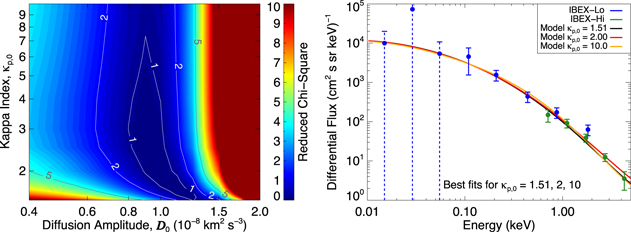
Figure 5. (Left) Reduced chi-square values calculated from comparing IBEX data with model ENA fluxes assuming the initial proton distribution fp,0 is a kappa function with free parameter κp,0. The diffusion coefficient spectral index is fixed at γ = 1.25, but the amplitude D0 varies. Note that the x and y axes are in log-scale. (Right) Model ENA fluxes for three best-fit cases: (1) κp,0 = 1.51, D0 = 1.25 × 10⁻⁸ km2 s−3, (2) κp,0 = 2, D0 = 1 × 10⁻⁸ km2 s−3, and (3) κp,0 = 10, D0 = 9 × 10⁻⁹ km2 s−3.
Download figure:
Standard image High-resolution imageThe right panel of Figure 5 shows three different ENA spectra when κp,0 = 1.51, 2, and 10, with different D0 that give the best fit to IBEX data in each case. While the reduced chi-square value is slightly better for κp,0 ≲ 7, one can see that even the case where κp,0 = 10 matches IBEX data reasonably well. Our results suggest that there is not sufficient resolution in IBEX data to determine the best κp,0; however, this may be possible with higher resolution measurements from the future Interstellar Mapping and Acceleration Probe (IMAP) mission (https://imap.princeton.edu). Nonetheless, we are able to determine that the diffusion coefficient is limited to the range ∼8 × 10⁻⁹ km2 s−3 ≲ D0 ≲ 1.3 × 10⁻⁸ km2 s−3.
So far, we have analyzed our model results under the assumption that the velocity diffusion rate in the heliotail is approximately proportional to v1.3. While this may be true if κp,0 ∼ 1.63, this may not be true for smaller or larger κp,0. Figure 6 shows results from comparing model ENA fluxes with IBEX data where the diffusion coefficient D(v) scales between v2/3 and v2, which can arise from isotropic Kolmogorov (e.g., Isenberg 1987) and anisotropic Goldreich–Sridhar (e.g., Goldreich & Sridhar 1995; Eichler 2014) turbulence, respectively. We vary the diffusion amplitude to demonstrate how the model compares to IBEX data under different diffusion rates. As one can see in the left panels of Figure 6, the minimum reduced chi-square slightly depends on κp,0. For small κp,0 near ∼1.5, it appears that D(v) ∝ v1.3 yields a slightly better fit to the data. This is clearer in the right panels of Figure 6 where we show ENA spectra for the best-fit cases when the diffusion spectral index γ = 0.67, 1.25, and 2. While the case for D(v) ∝ v1.3 appears to be slightly better at lower energies, the model results for D(v) ∝ v2/3 and v2 are approximately within the 1σ measurement uncertainties. Similar results occur for larger κp,0 (κp,0 = 2, 10). Thus, while we cannot constrain the best κp,0 with significant certainty, we find that a diffusion coefficient that scales between ∼v2/3 and ∼v2 is most consistent with IBEX data for any κp,0. In order to balance the diffusion rate, the coefficient amplitude D0 must be small (∼2–4 × 10⁻¹⁰ km2 s−3) if D(v) ∝ v2 and large (∼1.5–2 × 10⁻⁷ km2 s−3) if D(v) ∝ v2/3.

Figure 6. (Left) Reduced chi-square results from comparison between model results and IBEX data for κp,0 = 1.51, 2, and 10. (Right) Model ENA fluxes for best fits to IBEX data when γ = 0.67, 1.25, and 2. Blue dots in reduced chi-square plots represent the best-fit model results shown in the right panels (γmin).
Download figure:
Standard image High-resolution image4.2. Comparison of ENA Spectra from Different TS-processed Distributions
In this section, we compare model ENA fluxes for different proton distribution functions: fp,0 is represented by a kappa distribution (we assume κp,0 = 1.63 hereafter), a filled-shell distribution for PUIs, and a superposition of three Maxwell–Boltzmann distributions (see Table 1). We also vary the diffusion amplitude D0 around ∼10−8 km2 s−3 to illustrate how slight changes in D0 may affect the results. The results are shown in Figure 7. Figure 7(a) shows that while each model produces similar results for energies <1 keV, at higher energies they deviate. The model that assumes PUIs are described by a filled-shell distribution downstream of the TS (fMS) that produces too many ENAs at energies above ∼2 keV. This is also clear in the results shown by Zank et al. (2010) using a simplified transport model. In fact, this is independent of the diffusion coefficient amplitude (compare Figures 7(a)–(c)). If there is no velocity diffusion, this model would still produce too many ENAs above ∼2 keV and too few ENAs at lower energies. Thus, we can already see that this type of interaction at the TS is not realistic.
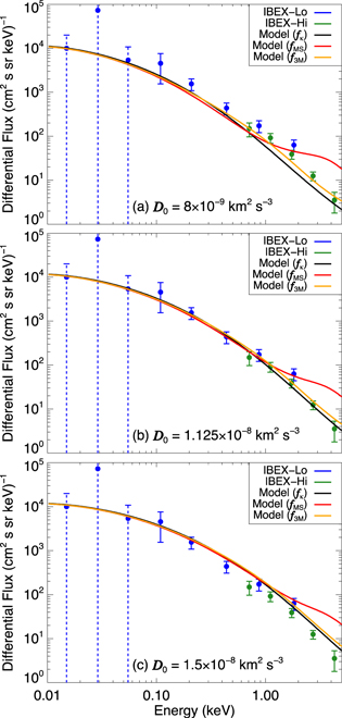
Figure 7. Model ENA fluxes for different initial proton distributions (fκ = kappa distribution with κp,0 = 1.63, fMS = core Maxwell–Boltzmann plus filled-shell, f3M = three Maxwell–Boltzmann distributions from Zank et al. 2010) and different diffusion amplitudes assuming D(v) ∝ v1.25.
Download figure:
Standard image High-resolution imageFor the case where the initial proton distribution is a superposition of three Maxwell–Boltzmann distributions representing core SW ions, PUIs transmitted across the TS, and PUIs reflected at the TS, the results are similar to the kappa distribution. By slightly varying D0, Figure 7 shows that it is possible to choose a different D0 to better fit either the fκ or f3M spectra to IBEX data, but in general they produce similar results. Moreover, the fact that both fκ and f3M can be used to reproduce IBEX data, but a filled-shell downstream distribution for PUIs (fMS) cannot, suggests that if PUIs are in a filled-shell distribution upstream of the TS, they most likely experience diffusion in energy via interactions with electromagnetic fluctuations at the ion kinetic scale at the TS, producing a smoother energy distribution than that assumed by Equation (8). We test this hypothesis in the next section.
4.3. Fully Kinetic Particle-in-cell Simulation of the Termination Shock
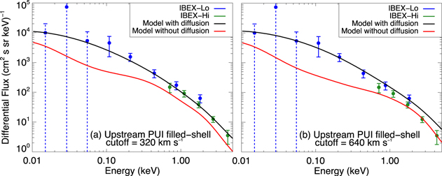
In the previous sections, we tested different analytic forms for the proton distribution function downstream of the TS, fp,0. However, based on the results in Section 4.2, if the PUI distribution upstream of the TS is a filled-shell, just heating the distribution at the TS according to Equation (8) is not realistic. Thus, we are motivated to test whether a more realistic derivation of fp,0 from an upstream filled-shell distribution can clarify how PUIs interact at the TS. To do this, we utilize the results of a fully kinetic PIC simulation of the TS from Kumar et al. (2018). This simulation utilizes data taken by Voyager 2 during its crossing of the TS in 2007 (Burlaga et al. 2008; Richardson et al. 2008) to constrain the upstream PUI distribution function. Kumar et al. (2018) showed that in order to reproduce Voyager 2 observations, including the compression ratio, energy partitioning, and magnetic field profile, the upstream PUI distribution can be represented by a filled-shell distribution, but with a cutoff approximately twice that of the SW flow speed just upstream of the TS (flow speed was ∼320 km s−1), such that the PUI mean energy is higher. They suggest that this is due to the increase in magnetic field observed by Voyager 2 within ∼1 au of the TS, resulting in the adiabatic compression and heating of PUIs.
While the properties of the TS at the location of Voyager 2 are not necessarily the same as in the downwind direction, and time variations in the SW make exact comparisons difficult, testing the results of Kumar et al. (2018) may offer a better prediction for the processing of PUIs at the TS, compared to the analytic functions described previously. We extract the proton distribution function downstream of the TS simulated by Kumar et al. (2018), binning all protons in speed bins used in our transport model (see the Appendix). The speed distributions that we test as boundary conditions in our model are shown in Figure 8, normalized such that the total density is 0.0017 cm−3. Figure 8(a) shows the downstream proton distribution in the case where the upstream PUI distribution was a filled-shell with cutoff at 320 km s−1 in the SW frame, i.e., the SW speed upstream of the TS at Voyager 2. Figure 8(b) is similar, except the upstream PUI filled-shell cutoff was 640 km s−1, which Kumar et al. (2018) suggested as a more appropriate form for the PUI distribution at the time and location of Voyager 2's crossing of the TS due to its higher mean energy. In the speed range ∼100–800 km s−1, corresponding to the IBEX energy range, the proton spectra are approximately power laws with speed slopes between −4 and −3.5. The distribution in Figure 8(b) has a shallower slope since more PUIs upstream of the TS exist at higher energies, and these PUIs are able to gain more energy at the TS (Kumar et al. 2018).
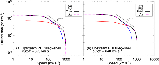
Figure 8. Proton distribution function downstream of the TS at Voyager 2 extracted from the fully kinetic PIC simulation of Kumar et al. (2018). Each panel shows the TS-processed distribution based on two different upstream conditions: the upstream PUI distribution was a filled-shell distribution with cutoff at (a) 320 km s−1 and (b) 640 km s−1. SW ions are shown in blue, PUIs in red, and the total distribution in black. We interpolate the total simulated distributions to our model speed grid (fp,0, dashed magenta), normalized such that the total density is 0.0017 cm−3.
Download figure:
Standard image High-resolution imageWe take the distributions shown in Figure 8 as fp,0 in our proton transport model, solve Equation (1), and calculate ENA fluxes at 1 au. We assume that the diffusion coefficient is proportional to v1.25, for consistency with our previous results. We also show the case when there is no diffusion in velocity. With no diffusion, the resulting ENA spectra for both initial distributions shown in Figure 8 are too low compared to IBEX data over most energies; interestingly, however, the 640 km s−1 upstream cutoff case matches the IBEX data above ∼2 keV even without velocity diffusion (Figure 9(b)). We find that the 320 km s−1 upstream cutoff case is consistent with IBEX data if D0 ∼ 8 × 10⁻⁹ km2 s−3 (Figure 9(a)), similar to the results presented in Section 4.1, but the other case cannot match IBEX data for any diffusion coefficient since it produces too many high energy ENAs. While we do not show the results for different diffusion spectral indices, it is clear that the PIC simulation results with an upstream filled-shell cutoff of 320 km s−1 can produce results consistent with our prior conclusion that the diffusion coefficient in the heliotail scales between v2/3 and v2.
Figure 9. Model ENA results using initial proton distributions derived from the PIC simulation from Figure 8. We assume the diffusion coefficient D(v) = 8 × 10⁻⁹ km2 s−3 (v/v0)1.25 for both (a) and (b) in black. We also show the case where D(v) = 0 in red.
Download figure:
Standard image High-resolution image
The fact that the downstream proton distribution that best matches the data from Voyager 2's observations at the TS fails to produce ENAs observed by IBEX from the heliotail may seem counterintuitive. However, this may indicate that (1) the long-term average of the proton distribution upstream of the TS should be a filled-shell with a cutoff at the SW speed, and that Voyager 2 observations represent an example of temporal variations about this average, or (2) the upstream PUI distribution as assumed by Kumar et al. (2018) is not strictly a filled-shell with higher speed cutoff, but possibly a filled-shell with cutoff at the upstream SW speed and a suprathermal, but relatively steep, tail at higher energies produced by particle interactions with turbulence farther upstream of the TS. This last possibility, as noted by Kumar et al. (2018), would still need to have a mean energy similar to that of a filled-shell with cutoff at 640 km s−1 in order to reproduce Voyager 2 observations.
4.4. Summary and Conclusions
In this study, we seek to understand how the functional form of the proton distribution processed by the TS in the downwind direction of the heliosphere (i.e., heliotail) affects ENA fluxes observed by IBEX at 1 au. By constraining the initial distribution function downstream of the TS with IBEX data, we may better understand how the TS processes PUIs, as well as understand the relative importance of energy-dependent processes occurring in the heliotail (charge exchange, adiabatic heating, and stochastic acceleration). We model IBEX ENA observations by solving the stationary Parker transport equation (Equation (1)) for the proton distribution in the heliotail assuming different functional forms for the proton distribution downstream of the TS. We include effects from charge exchange and adiabatic heating based on results from an MHD-plasma/kinetic-neutral simulation of the heliosphere, as well as a velocity diffusion term as a free parameter.
First, we test three analytic forms of the proton distribution function (fκ, fMS, f3M, see Table 1). We find that, while differences in the distributions are apparent close to the TS, at the speeds coinciding with the IBEX sensor's energy range (∼100–1000 km s−1) the distributions approach similar shapes after traveling a few hundred astronomical units from the TS due to the velocity diffusion term. As pointed out by Zirnstein et al. (2018b), a kappa distribution with index κp,0 = 1.63 does not significantly change with distance in the IBEX energy range since the best-fit diffusion rate approximately counteracts the loss of energetic protons by charge exchange. The other distributions, which are not initially smooth like the kappa distribution, change significantly over distance before smoothing in velocity space.
If the proton distribution downstream of the TS is a kappa distribution, we find that practically any initial kappa index in the range 1.51 ≤ κp,0 ≤ 10, where κp,0 = 10 is close to a Maxwell–Boltzmann distribution, is possible for a diffusion coefficient scaling close to ∼v1.3, with amplitude D0 ∼ 0.8–1.3 × 10⁻⁸ km2 s−3. While it appears that D(v) scaling close to v1.3 best reproduces IBEX data, a higher (D(v) ∝ v2) or lower (D(v) ∝ v2/3) diffusion rate may be possible within our uncertainties. A change from the widely known isotropic Kolmogorov (D(v) ∝ v2/3; e.g., Isenberg 1987) and anisotropic Goldreich–Sridhar (D(v) ∝ v2; e.g., Goldreich & Sridhar 1995; Eichler 2014) turbulence spectra suggests that the presence of PUIs, which constitute a significant fraction of the plasma density far from the TS, may be modifying the turbulence spectrum. We note also that particle interactions with compressive waves may also result in D(v) ∝ v2 (see e.g., Toptyghin 1980; Chalov et al. 2003; le Roux et al. 2005; Fahr et al. 2012; Zhang & Lee 2013).
We are not able to constrain the kappa index of the proton distribution function downstream of the TS due to the degeneracy between the kappa index and diffusion rate. However, a kappa index of less than 2 appears to be most probable based on earlier analyses of IBEX ENA observations (Livadiotis et al. 2011), as well as from Voyager observations of 0.04–4 MeV protons (Decker et al. 2005), and models of kappa distribution transport (e.g., Fahr et al. 2014, 2016). If this is the case, the average velocity diffusion amplitude in the heliotail likely lies in the range D0 ∼ 1–1.3 × 10⁻⁸ km2 s−3 for a diffusion rate that scales as D(v) ∝ v1.3.
A proton distribution constructed from a superposition of three Maxwell–Boltzmann distributions, commonly used to model multicomponent PUI distributions in the heliosheath (e.g., Zank et al. 2010), produces similar results to a kappa distribution. This is due to their similar initial shapes and processing by velocity diffusion. We also test a PUI filled-shell distribution that is compressed at the TS, producing a downstream filled-shell distribution with cutoff at large speed as proposed by Zank et al. (2010). We show that this distribution cannot reproduce IBEX observations, creating too many ENAs at ∼2–5 keV regardless of the diffusion rate in the heliotail. This is not a surprising result since more self-consistent models and simulations of particle interactions at quasi-perpendicular shocks show that PUIs experience diffusion in energy at the TS (e.g., Yang et al. 2015; Kumar et al. 2018), resulting in a smoother roll-over or tail rather than a sharp cutoff at higher energies. In fact, this was observed for the first time by the Solar Wind Around Pluto (SWAP) instrument on board New Horizons at an interplanetary shock ∼34 au from the Sun (Zirnstein et al. 2018c).
We test a more realistic processing of the PUI filled-shell distribution at the TS using the results from a fully kinetic PIC simulation from Kumar et al. (2018). First, we find that the PIC simulation produces a downstream distribution that, similar to the kappa and three Maxwell–Boltzmann distributions, cannot produce enough ENAs over most of the ENA spectrum without some form of velocity diffusion in the heliotail (see, however, Figure 9(b)). However, if the velocity diffusion coefficient in the heliotail does scale approximately as v1.3, then the most likely diffusion amplitude is approximately 8 × 10⁻⁸ km2 s−3 based on the PIC simulation results, which is similar to the results found earlier in this study (Sections 4.1–4.2) and by Zirnstein et al. (2018b). Interestingly, we find that a PUI filled-shell distribution with a large cutoff speed (here we tested a cutoff of 640 km s−1), as inferred by Kumar et al. (2018) to be more realistic than a cutoff at the SW speed in order to reproduce Voyager 2 observations of the TS, is inconsistent with IBEX observations of ENAs from the heliotail. This suggests either (1) that the long-term average of the proton distribution upstream of the TS could be a filled-shell with cutoff at the local SW speed and that Voyager 2 observations represent an instance of a temporal variation about this average, or (2) the upstream PUI distribution, as assumed by Kumar et al. (2018), is not strictly a filled-shell with higher speed cutoff, but possibly a filled-shell with cutoff at the upstream SW speed plus a suprathermal, but relatively steep, tail at higher energies.
Thus, our results suggest that the PUI distribution upstream of the TS can be a filled-shell like that suggested by Vasyliunas & Siscoe (1976), in agreement with recent observations from New Horizons' Solar Wind Around Pluto (SWAP; McComas et al. 2008) instrument, which showed that even out to 40 au from the Sun the PUI distributions can be quantified using the filled-shell function (though not necessarily representing physically meaningful parameters; McComas et al. 2017b). Moreover, IBEX ENA measurements substantiate recent SWAP observations of the preferential heating of PUIs at an interplanetary shock and the production of a suprathermal PUI tail downstream of the shock (Zirnstein et al. 2018c).
E.Z. and J.H. acknowledge support from NASA grant NNX16AG83G. R.K. was partially supported by the Max-Planck/Princeton Center for Plasma Physics and NSF grant AST-1517638. This work was also carried out as part of the IBEX mission, which is part of NASA's Explorer program. The work reported in this paper was performed at the TIGRESS High Performance Computing Center at Princeton University, which is jointly supported by the Princeton Institute for Computational Science and Engineering and the Princeton University Office of Information Technology's Research Computing department.
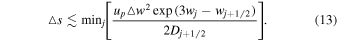
Appendix: Solving the Parker Transport Equation
We rewrite Equation (1) in natural logarithm space,
where w = ln(v). We solve for speeds in the plasma frame ranging from 1 to 10,000 km s−1, where the speed bin sizes range from ∼0.03 to 300 km s−1, respectively.
We solve Equation (11) using an explicit, "forward-time, central-difference" method, with a sufficiently small step size Δs. Equation (11) becomes (e.g., Press et al. 2002)
where n is the spatial (or time) step index (sn), j is the velocity step index (wj), Δs = sn+1 − sn, Δw = wj+1 − wj, Dj+1/2 = (Dj+1 + Dj)/2, Dj−1/2 = (Dj + Dj−1), wj+1/2 = (wj+1 + wj)/2, and wj−1/2 = (wj + wj−1)/2. We solve Equation (11) as a function of distance s = 0 to 800 au from the TS. The step size, Δs, is chosen such that it globally satisfies the stability condition, which is approximately given by (e.g., Press et al. 2002)